t t γ productioninthe e µ channelat13TeVwiththeATLASdetector ¯ Measurementsofinclusiveanddiﬀerentialcross-sectionsof ATLASCONFNote

(1)

A TLAS-CONF-2019-042 22 September 2019

ATLAS CONF Note

ATLAS-CONF-2019-042

22nd September 2019

Measurements of inclusive and differential

cross-sections of t t ¯ γ production in the eµ channel at 13 TeV with the ATLAS detector

The ATLAS Collaboration

Inclusive and differential cross-sections for the production of a top-quark pair in association with a photon are measured with proton-proton collision data corresponding to an integrated luminosity of 139 fb

⁻¹

. The data were collected by the ATLAS detector at the LHC during Run 2 between 2015 and 2018 at a centre-of-mass energy of 13 TeV. The measurements are performed in the top-quark pair eµ final state in a fiducial volume defined at parton level.

Events with exactly one photon, one electron and one muon of opposite sign, and at least two jets, out of which at least one is b -tagged, are selected. The fiducial cross-section is measured to be 44 . 2 ± 2 . 6 fb. Differential cross-sections as functions of several observables are compared to state-of-the-art Monte Carlo simulations and next-to-leading order theoretical calculations. These include cross-sections as functions of the photon transverse momentum and absolute pseudorapidity and angular variables related to the photon and the leptons and between the two leptons in the event. All measurements are in agreement with the predictions.

© 2019 CERN for the benefit of the ATLAS Collaboration.

Reproduction of this article or parts of it is allowed as specified in the CC-BY-4.0 license.

(2)

1 Introduction

Precise measurements of top-quark production and decay properties provide crucial information for testing the expectations of the Standard Model (SM) and its possible extensions. In particular, the study of the associated production of a top-quark pair ( t t ¯ ) with a photon probes the tγ electroweak coupling.

Furthermore, measurements of the inclusive and differential cross-sections of this process are of particular interest because these topologies are sensitive for instance to new physics through anomalous dipole moments of the top quark [1–3] and in the context of effective field theories (EFT) [4].

First evidence for the production of a top-quark pair in association with a photon ( t¯ tγ ) was reported by the CDF Collaboration [5], while the observation of the t tγ ¯ process was established by the ATLAS Collaboration in proton-proton ( pp ) collisions at

√ s = 7 TeV [6]. Both the ATLAS and CMS Collaborations measured the t tγ ¯ cross-section at

√ s = 8 TeV [7, 8]. The first measurements of the inclusive and differential cross-sections at

√ s = 13 TeV were performed by the ATLAS Collaboration [9].

This note presents a measurement of the fiducial inclusive and differential t tγ ¯ production cross-sections in the final state with one electron and one muon, referred to as the eµ channel. Events where the electrons and muons arise from the leptonic decays of τ -leptons are excluded. The measurement is performed using the full data set recorded at the LHC between 2015 and 2018 at a centre-of-mass energy of

√ s = 13 TeV and corresponding to an integrated luminosity of 139 fb

⁻¹

. The fiducial inclusive cross-section is measured using a likelihood fit to the distribution of S

_T

, defined as the scalar sum over all transverse momenta in the event, including leptons, photons, jets and missing transverse momentum. The differential cross-sections, absolute and normalised to unity, are measured in the same fiducial region as the inclusive cross-section, as functions of photon kinematic variables, angular variables related to the photon and the leptons, and angular separations between the two leptons in the event.

Compared to the previous t tγ ¯ ATLAS analysis with 13 TeV data [9], only the e µ channel is considered since it provides a clean final state with a small background contribution and, thus, no multivariate analysis techniques are needed to separate signal and background processes. Additionally, the cross-sections are measured at parton level instead of at particle level to be compared to the theory calculation in Ref. [10].

The calculation constitutes the first full computation for t t ¯ production with a final-state photon in hadronic collisions at next-to-leading order (NLO) in QCD, pp → bW bWγ , including all resonant and non-resonant diagrams, interferences, and off-shell effects of the top quarks and the W bosons.

The note is organised as follows. The ATLAS detector is briefly introduced in Section 2. Details of the event-simulation generators and their theoretical predictions are given in Section 3. The object and event selection and the analysis strategy are presented in Sections 4 and 5. The systematic uncertainties are described in Section 6. The results for the inclusive and differential cross-sections are presented in Sections 7 and 8, respectively. Finally, a summary is given in Section 9.

2 ATLAS detector

ATLAS [11–13] is a multipurpose detector with a forward–backward symmetric cylindrical geometry with respect to the LHC beam axis.

¹

The innermost layers consist of tracking detectors in the pseudorapidity

1

ATLAS uses a right-handed coordinate system with its origin at the nominal interaction point (IP) in the centre of the detector and the z -axis along the beam pipe. The x -axis points from the IP to the centre of the LHC ring, and the y -axis points upwards.

Cylindrical coordinates (r, φ ) are used in the transverse plane, φ being the azimuthal angle around the z -axis. The pseudorapidity

(3)

range |η| < 2 . 5. An additional silicon pixel layer, the insertable B-layer, was added between 3 and 4 cm from the beam line to improve b -hadron tagging [12, 13] for Run 2. This inner detector (ID) is surrounded by a thin superconducting solenoid that provides a 2 T axial magnetic field. It is enclosed by the electromagnetic and hadronic calorimeters, which cover |η | < 4 . 9. The outermost layers of ATLAS consist of an external muon spectrometer (MS) within |η| < 2 . 7, incorporating three large toroidal magnetic assemblies with eight coils each. The field integral of the toroids ranges between 2.0 and 6.0 Tm for most of the acceptance. The MS includes precision tracking chambers and fast detectors for triggering. A two-level trigger system [14] reduces the recorded event rate to an average of 1 kHz.

3 Signal and background modelling

The estimation of signal and background contributions relies on the modelling of these processes with simulated events. These simulated events are produced with Monte Carlo (MC) event generators and the response of the ATLAS detector is simulated [15] with Geant4 [16]. For some of the estimates of modelling uncertainties, the fast-simulation package AtlFast-II is used instead of the full detector simulation. Additional pp interactions from the same bunch crossing (pile-up) are generated with Pythia 8 [17, 18] using the set of tuned parameters called A2 [19] and the MSTW2008LO parton distribution functions (PDF) set [20]. Corrections derived from dedicated data samples are applied to the MC simulation to improve the agreement with data.

This analysis uses both inclusive samples, in which processes are generated at matrix-element (ME) level without explicitly including a photon in the final state, and dedicated samples, where photons are included in the ME level generation step. Dedicated samples with a photon in the ME are generated for the t tγ ¯ and Wtγ final states, as well as for Vγ processes with additional jets. Here, V denotes either a W or a Z boson. Although no photons are generated at ME level in the inclusive samples, radiation of photons is still accounted for by the showering algorithm. Combining inclusive and dedicated samples for the modelling of processes might result in double-counting photon radiation in certain phase-space regions.

As a consequence, an overlap-removal procedure is performed between inclusive and dedicated samples.

Photon radiation simulated at ME level in dedicated samples comes with higher accuracy than the photon radiation in the showering algorithm. On the other hand, kinematic cuts are applied to the kinematic properties of the photons at ME level in the dedicated samples. In the overlap-removal procedure, all events from the dedicated samples are kept while events from the inclusive samples are only considered if they do not contain a parton-level photon that fulfils the kinematic requirements of the dedicated sample of p

_T

(γ) > 15 GeV and ∆R(γ, `) > 0 . 2, where p

_T

(γ) is the photon’s transverse momentum and ∆R(γ, `) is the angular distance between the photon and any charged lepton.

The dedicated sample for the t tγ ¯ signal process is simulated using the MadGraph5_aMC@NLO generator (v2.33) [21] and the NNPDF2.3LO PDF set [22] at leading order (LO) in QCD. The events are generated as a doubly-resonant 2 → 7 process, that is, as e.g. pp → blνblνγ , and, thus, diagrams where the photon is radiated from the initial state (in case of quark-antiquark annihilation), intermediate top quarks, the b -quarks, the intermediate W bosons as well as the decay products of the W bosons are included. The photon was requested to have p

_T

> 15 GeV and |η| < 5 . 0 and the leptons satisfy |η| < 5 . 0. The ∆R between the photon and any of the charged particles among the seven final-state particles were required to be greater than 0.2. The top-quark mass in this and all other samples is set to 172.5 GeV. The renormalisation and

is defined in terms of the polar angle θ as η = − ln tan ( θ / 2 ) . Angular distance is measured in units of ∆R ≡ p

(∆η )

2

+ (∆φ )

2

.

(4)

the factorisation scales are set to 0.5 × Í

i

q

m

²_i

+ p

_T,i²

, where the sum runs over all the particles generated from the ME calculation. The event generation is interfaced to Pythia 8 (v8.212) using the A14 tune [23]

to model parton shower, hadronisation, fragmentation and underlying event. Heavy-flavour hadron decays are modelled with EvtGen [24]; this programme is used for all samples, except for those generated using the Sherpa MC programme.

The dedicated sample for the Wtγ process is generated with the MadGraph5_aMC@NLO generator as well. It also makes use of the NNPDF2.3LO PDF set and is interfaced to Pythia 8 (v8.212) for the showering using the A14 tune. The sample is produced at LO in the five-flavour scheme for the 2 → 3 process assuming a stable top quark. The photon is also required to have p

_T

> 15 GeV and |η| < 5 . 0 and to be separated by ∆R > 0 . 2 from any parton. To account for missing contributions of photons from radiative top-quark decays, the sample is reweighted in the photon p

_T

distribution at parton level to match a combined MadGraph5_aMC@NLO simulation of the Wtγ process including initial and final state radiation. At NLO, the Wtγ process interferes with the t¯ tγ signal process when including the spectator b -quark and would contribute to the off-shell part of the signal. Since the Wtγ process is generated at LO without the spectator b -quark from the initial state, the interference effects cannot be calculated. For this reason, Wtγ is treated as a background contribution in this analysis, although a small part of what is defined as signal in the theoretical cross-section calculation for the pp → bW bW γ process from Ref. [10]

might be missing.

Events with Wγ and Z γ final states (with additional jets) are simulated as dedicated samples. Wγ processes are simulated with Sherpa 2.2.2 [25, 26] at NLO accuracy in QCD using the NNPDF3.0NNLO PDF set, whereas Z γ events are generated with Sherpa 2.2.4 at LO in QCD. The samples are normalised to the cross-sections given by the corresponding MC simulation. The Sherpa generator performs all steps of the event generation, from the hard process to the observable particles. All samples are matched and merged by the Sherpa-internal parton showering based on Catani-Seymour dipoles [27, 28] using the MEPS@NLO prescription [29–31]. Virtual corrections for the NLO accuracy in QCD in the matrix element are provided by the OpenLoops library [32, 33].

Inclusive t t ¯ production processes are simulated at matrix-element level at NLO accuracy in QCD using Powheg-Box-v2 [34–36]. The calculation uses the NNPDF3.0NLO PDF set [37]. The parton shower is generated with Pythia 8 (v8.230), for which the A14 tune is used. The t t ¯ events are normalised to a cross-section value calculated with the Top++2.0 programme at next-to-next-to-leading order (NNLO) in perturbative QCD, including soft-gluon resummation to next-to-next-to-leading-logarithm order (see Ref. [38] and references therein).

Events with inclusive W - and Z -boson production in association with additional jets are simulated with Sherpa 2.2.1 [25, 26] at NLO in QCD. The NNPDF3.0NLO PDF set is used in conjunction with a dedicated tune provided by the Sherpa authors. The samples are normalised to the NNLO cross-section in QCD [39].

Events with two vector bosons, that is, WW , WZ and ZZ , are generated with Sherpa versions 2.2.2 (purely leptonic decays) and 2.2.1 (all others) at LO in QCD. The NNPDF3.0NNLO PDF set is used in conjunction with a dedicated tune provided by the Sherpa authors. The samples are normalised to NLO accuracy cross-sections in QCD [40].

Events with a t¯ t pair and an associated W or Z boson ( t tV ¯ ) are simulated at NLO ME level with

MadGraph5_aMC@NLO using the NNPDF3.0NLO PDF set. The ME generator is interfaced to Pythia 8

(5)

(v8.210), for which the A14 tune is used in conjunction with the NNPDF2.3LO PDF set. The samples are normalised to NLO in QCD and electroweak theory [41].

The background processes are sorted in three categories based on the origin of the reconstructed photon required in the event selection. The first category is labelled h-fake and contains any type of hadronic fakes that mimic a photon signature in the detector. This category includes photon signatures faked by hadronic energy depositions in the electromagnetic calorimeter, but also hadron decays involving photons, for example π

⁰

→ γγ decays. The processes falling into this category include t¯ t , W +jets, Z +jets, diboson and t tV ¯ production with an additional h-fake photon. It also includes processes with a prompt photon, where the prompt photon is not reconstructed in the detector or does not pass the selection requirements, but a h-fake photon does. The small contribution of h-fake photons in the eµ channel is estimated based on the MC simulation. Studies performed with data-driven techniques show that possible data-driven corrections have a negligible effect on the shape of relevant observables. Possible differences in the total expected number of events are covered by a normalisation uncertainty as described in Section 6. The e-fake category contains processes with an electron mimicking a photon signature in the calorimeter, including contributions from processes with an e-fake photon and no prompt photon, and processes with a prompt photon in the simulation, but an e-fake photon in the reconstruction. This category represents a minor background contribution and the simulation is used as well to predict it. The third category is called prompt γ background and contains any type of background process with a prompt photon. The background contribution from t t ¯ production with a photon produced in an additional pp interaction in the same bunch crossing is found to be negligible.

t¯ tγ events where one or both W bosons decay into τ -leptons, which then subsequently decay into e or µ , are categorised as Other t tγ ¯ , not as t¯ tγ eµ signal, following the definition of signal events in the theory calculation in Ref. [10]. Single-lepton events, where a second lepton is faked by hadronic energy depositions, are also included in the category Other t¯ tγ . The contribution of t tγ ¯ single-lepton events was found to be negligible in the eµ final state in the previous measurement [9] and it is therefore estimated from the MC simulation.

4 Event selection

The data set used in this analysis corresponds to the 139 fb

⁻¹

of integrated luminosity collected with the ATLAS detector during the Run 2 period. Each event in data and simulation is required to have at least one reconstructed primary vertex with at least two associated reconstructed tracks. Furthermore, only events where at least one of the single-electron [42] or single-muon triggers was fired are selected. The p

_T

threshold of the single-lepton triggers was increased over the different data-taking periods from 25 GeV in 2015 over 27 GeV in 2016 to 28 GeV in 2017 and 2018.

The main physics objects considered in this analysis are electrons, muons, photons, jets, b -jets and missing transverse momentum. Electrons are reconstructed from energy deposits in the electromagnetic calorimeter associated with reconstructed tracks in the ID system. They are identified with a combined likelihood technique [43] and are required to be isolated. The origin of the electron track has to be compatible with the primary vertex. Electrons are calibrated with the method described in Ref. [44]. They are selected if they fulfil p

_T

> 25 GeV and |η

_clus

| < 2 . 47, excluding the calorimeter crack region 1 . 37 < |η

_clus

| < 1 . 52.

²

2

η

_clus

denotes the pseudorapidity of the calorimeter cluster associated with the electron.

(6)

Muons are reconstructed with a combined algorithm, using the track segments in the various layers of the muon spectrometer and the tracks in the ID system. The reconstruction, identification and calibration methods are described in Ref. [45]. Only isolated muons with calibrated p

_T

> 25 GeV and |η| < 2 . 5 are considered. The muon track is also required to originate from the primary collision vertex.

Photons are reconstructed from energy deposits in the central region of the electromagnetic calorimeters.

If the cluster is considered not matched to any reconstructed tracks in the ID system, the photon candidate is classified as unconverted. If the cluster is matched with one or two reconstructed tracks that are consistent with originating from a photon conversion and if, in addition, a conversion vertex can be found, the photon candidate is classified as converted. Both kinds of photons are considered in this analysis.

Photons are reconstructed and identified as described in Ref. [46] and the energies are calibrated with the method described in Ref. [44]. They are also required to be isolated with an isolation cut defined as

E

_T^iso

_∆R<

0.4

< 0 . 022 · E

_T

(γ) + 2 . 45 GeV in conjunction with p

^iso

T

_∆R<

0.2

< 0 . 05 · E

_T

(γ) , where E

_T^iso

refers to the calorimeter isolation within ∆R < 0 . 4 in the direction of the photon candidate and p

^iso

T

is the track isolation within ∆R < 0 . 2. Only photons with calibrated E

_T

> 20 GeV and |η

_clus

| < 2 . 37, excluding the calorimeter crack region 1 . 37 < |η

_clus

| < 1 . 52, are considered.

The jets are reconstructed using the anti- k

_t

algorithm [47] in the FastJet implementation [48] with a distance parameter R = 0 . 4 (in the η - φ plane). They are reconstructed from topological calorimeter clusters [49]. The jet energy scale and jet energy resolution are calibrated following Ref. [50]. The jets are required to have p

_T

> 25 GeV and |η | < 2 . 5. In order to reject jets from pile-up or other primary vertices, candidates for such jets are identified with the Jet Vertex Tagger [51] and rejected.

The b -tagging algorithm to identify jets from b -quark hadronisation [52] is based on a boosted decision tree (BDT) combining information from other algorithms utilising the impact parameter, secondary vertices, and a multi-vertex reconstruction algorithm. A working point with an efficiency of 85% on simulated events is used. The flavour tagging efficiency of b -jets as well as of c - and light-jets is calibrated as described in Ref. [53].

The reconstructed missing transverse momentum E

^miss

T

[54] is computed as the negative vector sum over all reconstructed, fully calibrated physics objects including photons and remaining unclustered energy, also called soft terms . These soft terms are estimated from low- p

_T

tracks associated with the primary vertex not being assigned to any reconstructed object.

An overlap removal procedure is applied to avoid the reconstruction of the same energy clusters or tracks as different objects. First, electron candidates sharing their track with a muon candidate are removed and jets within a ∆R = 0 . 2 cone of a remaining electron are excluded. Secondly, electrons within a ∆R = 0 . 4 cone of the remaining jets are removed. If the distance between a jet and any muon candidate is ∆R < 0 . 4, the muon candidate is discarded if the jet has more than two associated tracks, otherwise the jet is removed.

Finally, photons within a ∆R = 0 . 4 cone of a remaining electron or muon are removed and the jets within a

∆R = 0 . 4 cone of a remaining photon are excluded.

Events are selected with exactly one electron and exactly one muon, each of which must carry p

_T

> 25 GeV.

At least one of these leptons has to be matched to a fired single-lepton trigger and has to fulfil the respective

p

_T

threshold of the trigger. Electrons and muons must have opposite sign charges and the eµ invariant

mass is required to be higher than 15 GeV. The event is required to have at least two jets and at least one of

the jets must be b -tagged. In addition, all events must contain exactly one reconstructed photon fulfilling

the condition that ∆R between the selected photon and any of the leptons is greater than 0.4.

(7)

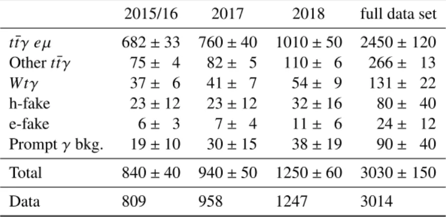
Table 1: The data and expected event yields before the likelihood fit for the signal and background processes after the full selection for the different data-taking periods and the full data set. All categories are estimated based on MC simulation including correction factors for detector effects as described in Section 6. The quoted uncertainties correspond to the total statistical and systematic uncertainties (cf. Section 6) added in quadrature.

2015/16 2017 2018 full data set t¯ tγ eµ 682 ± 33 760 ± 40 1010 ± 50 2450 ± 120 Other t tγ ¯ 75 ± 4 82 ± 5 110 ± 6 266 ± 13

Wtγ 37 ± 6 41 ± 7 54 ± 9 131 ± 22

h-fake 23 ± 12 23 ± 12 32 ± 16 80 ± 40

e-fake 6 ± 3 7 ± 4 11 ± 6 24 ± 12

Prompt γ bkg. 19 ± 10 30 ± 15 38 ± 19 90 ± 40 Total 840 ± 40 940 ± 50 1250 ± 60 3030 ± 150

Data 809 958 1247 3014

The pre-fit expected and observed event yields after selection are listed in Table 1 for the different signal and background categories described in Section 3. The table also includes expected and observed values for the different data-taking periods 2015/16, 2017 and 2018. Correction factors for detector effects (described in Section 6) are applied, when needed, to improve the description of the data by the simulation.

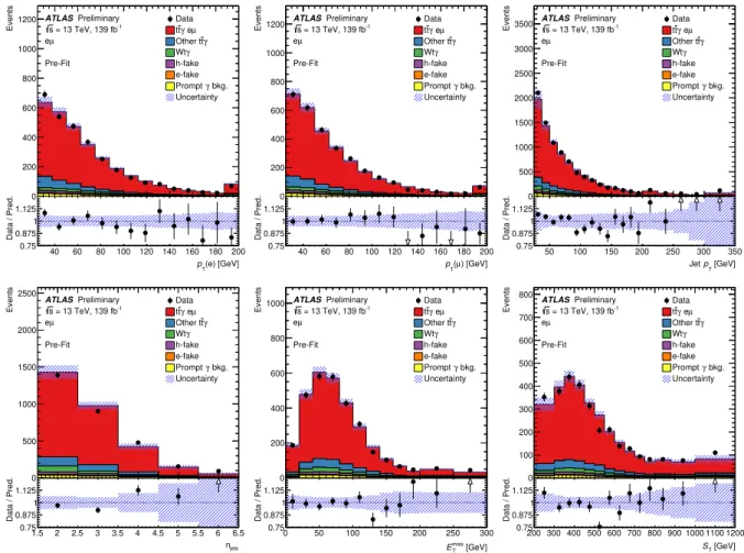
The modelling of signal and background is inspected through the comparison of distributions. A selection of these distributions showing a comparison between the MC simulation before the likelihood fit and data is presented in Figure 1. All systematic uncertainties that are introduced in Section 6 are included in these distributions and their quadratic sum is illustrated by the shaded error bands. The uncertainties cover almost all discrepancies observed between data and simulations.

5 Analysis strategy

The inclusive and differential cross-sections are measured in the fiducial region described in Section 5.1 and the same strategy for the estimation of the background contributions and systematic uncertainties is followed. In the inclusive cross-section the S

_T

distribution is fitted and the post-fit background yields and systematic uncertainties are used, while in the differential cross-sections no fit is performed.

5.1 Fiducial region definition

The cross-sections are reported at parton level in a fiducial region, defined by the kinematic properties of

the t¯ tγ process, in which all selected final-state objects are produced within the detector acceptance and

are thus measurable experimentally. This is done in a way that mimics the event selection as defined in the

theoretical calculation. Objects at parton level are taken from the MC simulation history. Photons and

leptons are selected as stable particles after final state radiation. The leptons ( ` = e, µ ) must originate from

W -boson decays and they are dressed with close-by photons within a cone of radius of R = 0 . 1 around

them and must have p

_T

> 25 GeV and |η| < 2.5. Only events with exactly one electron and one muon are

considered. Events with leptons originating from an intermediate τ -lepton in the top-quark decay chain

(8)

40 60 80 100 120 140 160 180 200 (e) [GeV]

pT

0.75 0.875 1 1.125

Data / Pred.

0 200 400 600 800 1000 1200

Events

ATLASPreliminary = 13 TeV, 139 fb-1

s eµ Pre-Fit

Data eµ tγ t

tγ Other t Wtγ h-fake e-fake

bkg.

Prompt γ Uncertainty

40 60 80 100 120 140 160 180 200 ) [GeV]

(µ pT

0.75 0.875 1 1.125

Data / Pred.

0 200 400 600 800 1000

Events1200

s eµ Pre-Fit

Data eµ tγ t

bkg.

50 100 150 200 250 300 350

[GeV]

pT

Jet 0.75

0.875 1 1.125

Data / Pred.

0 500 1000 1500 2000 2500 3000

Events3500

s eµ Pre-Fit

Data eµ tγ t

bkg.

1.5 2 2.5 3 3.5 4 4.5 5 5.5 6 6.5

njets

0.75 0.875 1 1.125

Data / Pred.

0 500 1000 1500 2000 2500

Events

s eµ Pre-Fit

Data eµ tγ t

bkg.

0 50 100 150 200 250 300

[GeV]

miss

ET

0.75 0.875 1 1.125

Data / Pred.

0 200 400 600 800

Events1000

s eµ Pre-Fit

Data eµ tγ t

bkg.

200 300 400 500 600 700 800 900 1000 1100 1200 [GeV]

ST

0.75 0.875 1 1.125

Data / Pred.

0 100 200 300 400 500 600 700 800

Events

s eµ Pre-Fit

Data eµ tγ t

bkg.

Figure 1: Distributions of the transverse momentum of the electron, the muon and all jets (top row), and the number of jets, E

^miss

T

and S

_T

(bottom row) after event selection and before the likelihood fit. The shaded bands correspond to the statistical and systematic uncertainties (cf. Section 6) added in quadrature. Underflow and overflow events are included in the first and last bins of the distributions, respectively.

are not considered. The b -jets at parton level in the calculation from Ref. [10] are jets clustered with the anti- k

_t

algorithm with a radius of R = 0 . 4. Since showering and hadronisation effects are not considered in this calculation, the jets correspond to the b -quarks from the top quark decay (with an additional parton in the cases where the NLO real emission leads to a parton close by a b -quark). To mimic this definition in the LO MC simulation, parton-level b -jets are defined as follows. The anti- k

_t

algorithm with a distance parameter R = 0 . 4 is applied on all partons that are radiated from the two b -quarks (including the b -quarks themselves) and from the two initial partons. The jets that include a b -quark from the decay of a top quark are selected as b -jets. The event is kept if there are two b -jets satisfying p

_T

> 25 GeV and |η| < 2 . 5.

Exactly one photon with E

_T

> 20 GeV and |η | < 2 . 37 is required. No photon-isolation requirement is

explicitly imposed at parton level; in the generation of the events at the ME level, the photon is required to

be separated by ∆R > 0 . 2 from any parton. The event is dropped if any of the following requirements is

not fulfilled: ∆R(γ, `) > 0 . 4, ∆R(e, µ) > 0 . 4, ∆R(b, b) ¯ > 0 . 4 or ∆R(`, b) > 0 . 4.

(9)

5.2 Fiducial inclusive cross-section

The fiducial inclusive cross-section is extracted using a profile likelihood fit to the S

_T

distribution. The expected signal and background distributions are modelled in the fit using template distributions constructed from the simulated samples. The parameter of interest, the fiducial cross-section σ

_fid

, is related to the number of signal events in bin i of the S

_T

distribution as:

N

_i^s

= L × σ

_fid

× C × f

_i^S^T

.

L is the integrated luminosity, f

_i^S^T

is the fraction of signal events falling into bin i of the S

_T

distribution, and C is the correction factor for the signal efficiency and for migration into the fiducial region f

_out

, defined as follows:

f

_out

= N

^non-fid

reco

N

_reco

, = N

^fid

reco

N

^fid

MC

⇒ C =

1 − f

_out

= N

_reco

N

^fid

MC

,

where N

_reco

is the simulated number of signal events passing the event selection described in Section 4, and N

^fid

MC

is the corresponding number of signal events generated in the fiducial region defined in Section 5.1.

The efficiency and outside migration are obtained from simulated t¯ tγ events. The correction factor is calculated to be C = 0 . 393 ± 0 . 013, where the uncertainty includes all signal modelling uncertainties (cf.

Section 6).

The likelihood function L , based on Poisson statistics, is given by:

L = Ö

i

P(N

_i^obs

|N

_i^s

( ® θ) + Õ

b

N

_i^b

( ® θ )) × Ö

t

G( 0 |θ

t

, 1 ).

N

_i^obs

, N

_i^s

, and N

_i^b

are the observed number of events in data, the predicted number of signal events, and the estimated number of background events in bin i of the S

_T

distribution, respectively. Also the rates of those t¯ tγ events not counted as part of the signal and categorised as Other t tγ ¯ are scaled with the same parameter as the signal events in the fit, that is, no independent production cross-section is assumed for these parts of the simulated t tγ ¯ process. The term θ ® represents the nuisance parameters that describe the sources of systematic uncertainties. Each nuisance parameter θ

_t

is constrained by a Gaussian distribution, G( 0 |θ

_t

, 1 ) . The width of the Gaussian corresponds to a change of ± 1 standard deviation of the corresponding quantity in the likelihood. For systematic uncertainties related to the finite number of simulated MC events, the Gaussian terms in the likelihood are replaced by Poisson terms. Each systematic uncertainty affects N

_i^s

and N

_i^b

in each bin of the distribution. The cross-section is measured by profiling the nuisance parameters and maximising this likelihood.

5.3 Normalised and absolute differential cross-sections

The measurements of the normalised and absolute differential cross-sections are performed as functions of

the p

_T

and |η| of the photon, and of angular variables between the photon and the leptons: ∆R between the

photon and the closest lepton ∆R(γ, `)

_min

, as well as ∆φ(`, `) and |∆η(`, `)| between the two leptons. The

kinematic properties of the photon are sensitive to the tγ coupling. In particular, ∆R(γ, `)

_min

is related

to the angle between the top quark and the radiated photon which can give insight into the structure of

this coupling. The distributions of ∆φ(`, `) and |∆η(`, `)| are sensitive to the t t ¯ spin correlation. The

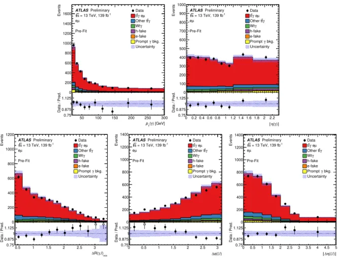
corresponding distributions in data compared to the SM simulations are shown in Figure 2.

(10)

50 100 150 200 250 300 ) [GeV]

(γ pT

0.75 0.875 1 1.125

Data / Pred.

0 200 400 600 800 1000 1200 1400

Events1600

s eµ Pre-Fit

Data eµ tγ t

bkg.

0 0.2 0.4 0.6 0.8 1 1.2 1.4 1.6 1.8 2 2.2 ) (γ η 0.75

0.875 1 1.125

Data / Pred.

0 100 200 300 400 500 600 700 800 900 1000

Events

s eµ Pre-Fit

Data eµ tγ t

bkg.

0.5 1 1.5 2 2.5 3

)min

l , γ R(

∆ 0.75

0.875 1 1.125

Data / Pred.

0 200 400 600 800 1000 1200

Events

s µ e Pre-Fit

Data µ e γ t t

bkg.

γ Prompt Uncertainty

0 0.5 1 1.5 2 2.5 3

) l,l ( φ

∆ 0.75

0.875 1 1.125

Data / Pred.

0 200 400 600 800 1000 1200 1400

Events

s µ e Pre-Fit

Data µ e γ t t

bkg.

0 0.5 1 1.5 2 2.5 3 3.5 4 4.5 5

) l,l ( η

∆ 0.75

0.875 1 1.125

Data / Pred.

0 200 400 600 800 1000 1200 1400

Events

s µ e Pre-Fit

Data µ e γ t t

bkg.

Figure 2: Distributions of the photon p

_T

and |η| in the top row, and ∆R(γ, `)

_min

, ∆φ(`, `) and |∆η(`, `)| in the bottom row after event selection and before the likelihood fit. The shaded bands correspond to the statistical and systematic uncertainties (cf. Section 6) added in quadrature. Underflow and overflow events are included in the first and last bins of the distributions, respectively.

The data are corrected for detector resolution and acceptance effects to parton level in the fiducial phase space using an iterative Bayesian unfolding procedure [55] implemented in the RooUnfold package [56].

The differential cross-section is defined as:

dσ

dX

_k

= 1

L × ∆X

_k

×

_k

× Õ

j

M

⁻_jk¹

× (N

_j^obs

− N

_j^b

) × ( 1 − f

_out_,_j

) .

The indices j and k represent the bin indices of the observable X at detector and parton levels, respectively.

The variable N

_j^obs

is the number of observed events, and N

_j^b

is the number of estimated background events

(pre-fit) in bin j at detector level. The efficiency

k

is the fraction of signal events generated at parton level

in bin k of the fiducial region, that are reconstructed and selected at detector level. L corresponds to the

total integrated luminosity and ∆X

_k

represents the bin width. The migration matrix M

_{k j}

describes the

detector response and expresses the probability for an event in bin k at parton level to be reconstructed

in bin j at detector level, calculated from events passing both the fiducial-region selection and the event

selection. The outside-migration fraction f

_out_,_j

is the fraction of signal events generated outside the fiducial

region but reconstructed and selected in bin j at detector level. The normalised differential cross-section is

derived by dividing the absolute result by the total cross-section, obtained by integrating over all bins of

(11)

the observable.

The estimated number of background events from processes other than t tγ ¯ production is subtracted from the number of events in data. The contribution from the Other t tγ ¯ category is taken into account by correcting the remaining number of observed events by the signal fraction, defined as the ratio of the number of selected t tγ ¯ signal events to the total number of selected t tγ ¯ events, as determined from simulation. This avoids the dependence on the inclusive signal cross-section used for the normalisation.

The signal MC samples are used to determine

_k

, f

_out_,_j

, and M

_{k j}

. The unfolding method relies on the Bayesian probability formula to invert the migration matrix, starting from a given prior of the parton-level distribution and iteratively updating it with the posterior distribution. The binning choices of the unfolded observables take into account the detector resolution and the expected statistical uncertainty. The bin width has to be larger than twice the resolution, and the statistical uncertainty is required to be around or below 10% across all bins, with the latter being the dominant factor. The resolution of the lepton and photon momenta is very high and, therefore, the fraction of events migrating from one bin to another is extremely small. In all bins, the purity, defined as the fraction of reconstructed events that originate from the same bin, is larger than 70%, and it is above 90% for all observables except for the p

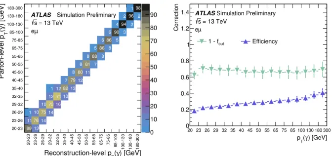
_T

of the photon. The number of iterations chosen is two, which provides good convergence of the unfolding distribution and a statistically stable result. For illustration purposes, the migration matrix, the efficiency, and the outside-migration fraction obtained for the distribution of the photon p

_T

are presented in Figure 3. The performance of the unfolding procedure is tested for possible biases from the choice of the input model. It has been verified that by reweighting the shape of the signal simulation by up to 50% with respect to the nominal shape, the unfolding procedure based on the nominal response matrix reproduces the altered shapes within the statistical uncertainties.

0 10 20 30 40 50 60 70 80 90

88 13 11 76 14

1 10 75 14 10 73 16

12 71 10 1 12 82 13

7 79 12 8 80 11

8 81 7 8 88 8

5 86 8 6 86 5

6 90 3 4 94 2

2 96 2 1 98

20-23 23-26 26-29 29-32 32-35 35-40 40-45 45-50 50-55 55-65 65-75 75-85 85-100 100-130 130-180 180-300

) [GeV]

( γ Reconstruction-level p

T 20-23

23-26 26-29 29-32 32-35 35-40 40-45 45-50 50-55 55-65 65-75 75-85 85-100 100-130 130-180 180-300

) [GeV] γ (

T

Parton-level p

ATLAS Simulation Preliminary

= 13 TeV s

e µ

) [GeV]

( γ p

T

Correction

0 0.2 0.4 0.6 0.8 1 1.2

1.4 ATLAS Simulation Preliminary = 13 TeV

s e µ

1 - f

out

Efficiency

20 23 26 29 32 35 40 45 50 55 65 75 85 100 130 180 300

Figure 3: Left: migration matrix relating the photon p

_T

at the reconstruction and parton levels in the fiducial phase

space, normalised by column and shown as percentages. Right: signal reconstruction and selection efficiency ( ) and

(1 − f

out

) fraction as a function of the photon p

_T

.

(12)

6 Systematic uncertainties

Different sources of systematic uncertainties are considered arising from detector effects, as well as theoretical uncertainties. Signal and background predictions are subject to these uncertainties.

6.1 Experimental uncertainties

Experimental systematic uncertainties affect the normalisation and shape of the distributions of the simulated signal and background samples. These include reconstruction and identification efficiency uncertainties, as well as uncertainties on the energy and momentum scale and resolution for the reconstructed physics objects in the analysis, including leptons, photons, jets and E

^miss

T

. In addition, uncertainties on flavour-tagging of jets, the jet vertex fraction (JVT), the integrated luminosity value and the pile-up simulation are considered.

The photon identification and isolation efficiencies as well as the efficiencies of the lepton reconstruction, identification, isolation, and trigger in the MC samples are all corrected to match the corresponding values in data. Similarly, corrections to the lepton and photon momentum scale and resolution are applied in simulation [44, 45]. All these corrections, which are p

_T

and η dependent, are varied within their uncertainties to study their impact on the final results.

The jet energy scale (JES) uncertainty is derived using a combination of simulations, test-beam data and in-situ measurements [50]. Additional contributions from jet-flavour composition, η -intercalibration, punch-through, single-particle response, calorimeter response to different jet flavours, and pile-up are taken into account, resulting in 30 uncorrelated JES uncertainty subcomponents. The jet energy resolution (JER) in simulation is smeared up by the measured JER uncertainty [57]. The uncertainty associated with the JVT cut is obtained by varying the efficiency correction factors.

The uncertainties related to the b -jet tagging calibration are determined separately for b -jets, c -jets and light-jets [58–60]. The corrections are varied by their measured uncertainties.

The uncertainties associated with energy scales and resolutions of photons, leptons and jets are propagated to the E

^miss

T

. Additional uncertainties originate from the modelling of its soft term [61].

The uncertainty in the combined 2015–2018 integrated luminosity is 1.7% [62], obtained using the LUCID-2 detector [63] for the primary luminosity measurements.

The uncertainty associated to the modelling of pile-up in the simulation is assessed by varying the reweighting of the pile-up in the simulation within its uncertainties.

6.2 Signal and background modelling uncertainties

The t¯ tγ signal modelling uncertainties include the uncertainties owing to the choice of the QCD scales, the

parton shower, the amount of initial state radiation (ISR) and the PDF set. The QCD scale uncertainty is

evaluated by varying the renormalisation and factorisation scales up and down by a factor of two from their

nominal choices simultaneously. The uncertainty on the parton shower and hadronisation is estimated

by comparing the t tγ ¯ nominal samples, produced with MadGraph5_aMC@NLO + Pythia 8, with an

alternative sample interfaced to Herwig 7. The ISR uncertainty is studied by comparing the variations of

the A14 tune parameter for radiation with its nominal values in the MadGraph5_aMC@NLO + Pythia 8

(13)

sample [23]. The PDF uncertainty is evaluated using the standard deviation of the distribution formed by the set of 100 replicas of the NNPDF set [22].

For the Wtγ process the uncertainties on the renormalisation and factorisation scales are also estimated by varying them up and down by a factor of two with respect to the nominal sample value simultaneously.

A systematic uncertainty on the parton shower and hadronisation model is considered by comparing Pythia 8 and Herwig 7 both interfaced to MadGraph5_aMC@NLO. To account for possible uncertainties resulting from the reweighting applied to the Wtγ simulation, an additional uncertainty is assigned:

a second reweighting is constructed for the Wtγ contribution to the S

_T

distribution. The difference between this closure-based reweighting and the reweighting parameterised in photon p

_T

is taken as as a shape-only uncertainty on the Wtγ prediction. An additional uncertainty of ± 15% is assigned to the normalisation of Wtγ , based on the theoretical uncertainties on the Wtγ fiducial cross-section from the MadGraph5_aMC@NLO simulation.

Several uncertainties of the modelling of t¯ t processes, which contribute to the h-fake and prompt γ background categories, are considered as shape-only uncertainties. The uncertainty on the matrix-element generation is estimated by comparing the nominal Powheg + Pythia 8 simulation with an alternative MadGraph5_aMC@NLO + Pythia 8 sample. The uncertainties on the parton shower and hadronisation are estimated by comparing the nominal simulation with alternative showering by Herwig 7. Uncertainties on ISR are estimated by comparing the nominal Powheg + Pythia 8 simulation against two sets of event weights produced with higher and lower radiation parameter settings in the A14 tune.

In addition to those background modelling uncertainties, 50% global normalisation uncertainties are assigned to the three categories h-fake photons, e-fake photons and prompt γ background [9].

6.3 Treatment of the systematic uncertainties in the measurements

As stated in Section 5, the impact of systematic uncertainties on the inclusive cross-section measurement is taken into account via nuisance parameters in the likelihood function. The nuisance parameters θ ® are profiled in the likelihood fit.

To avoid high sensitivity to statistical fluctuations due to the limited number of events of the MC samples used in systematic variations, smoothing techniques are applied to the MC templates used to evaluate the signal and background modelling systematic uncertainties in the template fit. Additionally, the systematic uncertainties are symmetrised, taking the average of the up- and down-variation as the uncertainty. In the cases where both variations have the same sign or only one variation is available (e.g. uncertainty on the parton shower and hadronisation signal modelling) the largest variation or the available one, respectively, is taken as both the up- and down-variations for the corresponding source.

In the case of the differential cross-section measurement, the pre-fit systematic variations are used for

the study since the measurement is still dominated by statistical uncertainties. The same symmetrisation

approach described for the inclusive cross-section is used for this measurement. Each systematic

uncertainty is determined individually in each bin of the measurement by varying the corresponding

efficiency, resolution, and model parameter within its uncertainty. For each variation, the measured

differential cross-section is recalculated and the difference with respect to the nominal result is taken

as the systematic uncertainty. The overall uncertainty in the measurement is then derived by adding all

contributions in quadrature, assuming the sources of systematic uncertainty to be fully uncorrelated.

(14)

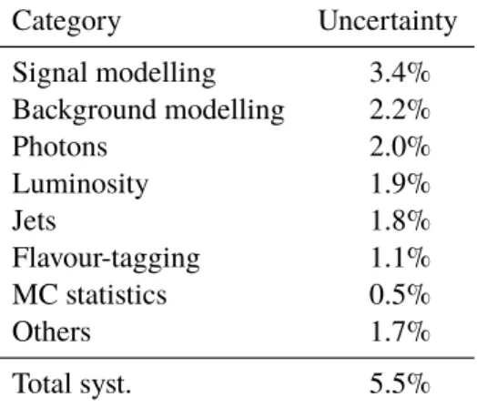
Table 2: Systematic uncertainties grouped into different categories and their relative impact on the measurement of the inclusive fiducial cross-section. The categories “Signal modelling” and “Background modelling” include all corresponding systematic uncertainties described in Section 6.2. The category “Photons” corresponds to the uncertainties related to photon identification and isolation. “Jets” includes the total JES, JER and JVT cut uncertainty, while the b -tagging related uncertainties are given in a separate category (“Flavour-tagging”). All remaining experimental uncertainties except for luminosity are included in the category “Others”.

Category Uncertainty

Signal modelling 3.4%

Background modelling 2.2%

Photons 2.0%

Luminosity 1.9%

Jets 1.8%

Flavour-tagging 1.1%

MC statistics 0.5%

Others 1.7%

Total syst. 5.5%

Sources of systematic uncertainty related only to the background prediction are evaluated by shifting the nominal distribution of the corresponding background process by its associated uncertainty. For the experimental uncertainties, the input is varied by the corresponding shift, which typically affects both shape and normalisation of signal and background processes. The resulting distribution is unfolded and compared with the nominal unfolded distribution. The systematic uncertainties due to signal modelling are evaluated by varying the signal corrections, that is, the migration matrix M

_{k j}

, the efficiency

_k

and the fraction f

_out_,_j

, and calculating the difference of the resulting unfolded distributions with respect to the nominal results.

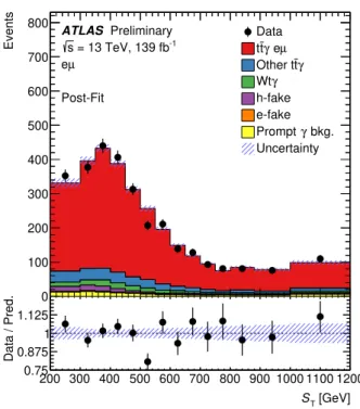
7 Inclusive cross-section measurement

The inclusive t tγ ¯ cross-section is extracted using a profile likelihood fit to the S

_T

distribution and it is extrapolated to the fiducial phase space given by the kinematic boundaries of the t¯ tγ signal as described in Section 5.

Table 2 lists the systematic uncertainties and their relative impact on the measurement of the inclusive cross-section. The effect of each category of uncertainties is calculated from the quadratic difference between the total uncertainty in the measured fiducial cross-section and the uncertainty from the fit with the corresponding nuisance parameters fixed to their fitted values. The uncertainties on the signal modelling, especially the t¯ tγ showering uncertainty, have the largest impact on the result.

The best fit values of the nuisance parameters correspond to variations that for most of the parameters are within one standard deviation of the prior uncertainties. The fit constrains slightly some of the nuisance parameters, for instance the t¯ tγ showering and the t¯ t ME uncertainty, resulting in uncertainties 20 to 40%

smaller than their initial values. The distribution of the fitted S

_T

variable is shown in Figure 4. The dashed band represents the post-fit uncertainties. The expected yields after the fit describe the data well.

Extrapolated to the fiducial phase space using the correction factor C , the fit result corresponds to an inclusive

cross-section for the t¯ tγ process in the eµ channel of σ = 44 . 2 ± 0 . 9 (stat)

⁺²₋₂^._.⁶₄

(syst) fb = 44 . 2 ± 2 . 6 fb. The

(15)

200 300 400 500 600 700 800 900 1000 1100 1200 [GeV]

ST

0.75 0.875 1 1.125

Data / Pred.

0 100 200 300 400 500 600 700 800

Events

ATLAS Preliminary = 13 TeV, 139 fb-1

s eµ Post-Fit

Data eµ tγ t

bkg.

Figure 4: Post-fit distribution of the S

_T

variable. The uncertainty band represents the post-fit uncertainties. Underflow and overflow events are included in the first and last bins of the distribution, respectively.

measured cross-section is slightly larger than the dedicated theoretical calculation provided by the authors of Ref. [10], which predicts a value of σ = 39 . 50

⁺⁰₋₂^._.⁵⁶₁₈

(scale)

⁺¹₋₁^._.⁰⁴₁₈

(PDF) fb for the chosen fiducial phase space using the CT14 PDF set [64]. The uncertainty on the theory prediction includes uncertainties owing to the scales and PDF. The PDF uncertainty is rescaled to the 68% CL. In the theoretical calculation, the renormalisation and factorisation scales are chosen as H

_T

/4, where H

_T

is the total transverse momentum of the system, defined as the scalar sum of the p

_T

of the leptons, b -jets, photon and the total missing p

_T

from the neutrinos. The mass of the top quark is set to 173.2 GeV. The electroweak coupling in the calculation is derived from the Fermi constant G

_µ

and it is set to α

_G_µ

≈ 1 / 132, while it is 1/137 for the leading emission.

Further details can be found in Ref. [10].

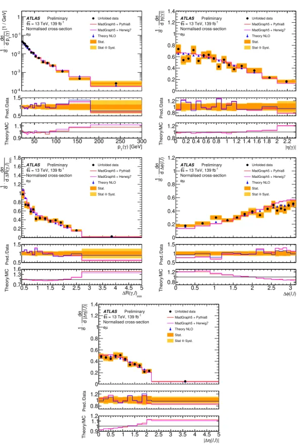
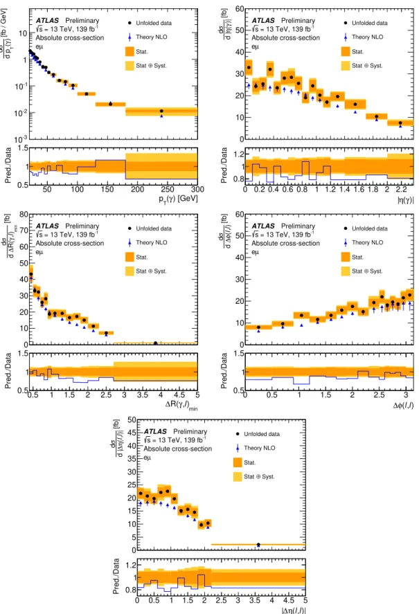
8 Differential cross-section measurements

The normalised differential cross-sections are shown in Figure 5 while the absolute measured differential

cross-sections are presented in Figure 6. The cross-sections are compared to the NLO calculation in the

same fiducial phase space and to the LO MadGraph5_aMC@NLO simulation (2 → 7 process) interfaced

with Pythia 8 and Herwig 7. The impact on the shape of the considered observables of the missing

Wtγ contribution in the signal definition is expected to be small. The shape of the measured differential

distributions is generally well described by both, the LO MC predictions from MadGraph5_aMC@NLO as

well as the NLO theory prediction. The latter tends to describe the shape of the measured distribution slightly

better. The shape of the ∆ φ(`, `) is not perfectly modelled by the MadGraph5_aMC@NLO simulation,

while the NLO prediction provides a better description of this distribution. The calculated χ

²

/ndf values

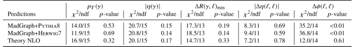
for the normalised and absolute cross-section and their corresponding p-values are summarised in Tables 3

(16)

Table 3: χ

²

/ndf and p -values between the measured normalised cross-sections and various predictions from the MC simulation and the NLO calculation.

pT(γ) |η(γ) | ∆R(γ, `)_min |∆η(`, `) | ∆φ(`, `)

Predictions χ²/ndf p-value χ²/ndf p-value χ²/ndf p-value χ²/ndf p-value χ²/ndf p-value MadGraph+Pythia8 14.0/15 0.53 20.7/15 0.15 17.3/13 0.19 8.3/11 0.69 35.2/14 <0.01 MadGraph+Herwig7 11.9/15 0.69 20.8/15 0.14 18.5/13 0.14 9.4/11 0.59 36.8/14 <0.01

Theory NLO 16.9/15 0.32 20.1/15 0.17 14.7/13 0.33 7.2/11 0.78 12.0/14 0.61

Table 4: χ

²

/ndf and p -values between the measured absolute cross-sections and the NLO calculation.

pT(γ) |η(γ) | ∆R(γ, `)_min |∆η(`, `) | ∆φ(`, `)

Predictions χ²/ndf p-value χ²/ndf p-value χ²/ndf p-value χ²/ndf p-value χ²/ndf p-value Theory NLO 16.0/16 0.45 20.7/16 0.19 12.8/14 0.54 11.4/12 0.49 16.3/15 0.36

and 4, quantifying the compatibility between data and each of the predictions. The χ

²

values are calculated as: χ

²

= (σ

_j,_data

− σ

_j,_pred.

) · C

⁻_jk¹

· (σ

_k,_data

− σ

_k,_pred.

) ,

where σ

_data

and σ

_pred.

are the unfolded and predicted differential cross-sections, C

_jk

is the covariance matrix of σ

_data

, calculated as the sum of the covariance matrix for the statistical uncertainty and the covariance matrices for each of the systematic uncertainties, and j and k are the binning indices of the distribution.

The covariance matrix for each of the systematic uncertainties is estimated as σ

_j

× σ

_k

, where σ

_j

and σ

_k

are the symmetrised uncertainties for bin j and bin k of the unfolded distribution. In the case of the normalised differential cross-sections, the last bin is removed from the χ

²

calculation and the number of degrees of freedom is reduced by one.

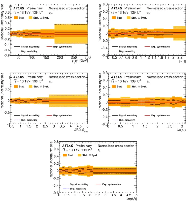
The systematic uncertainties of the unfolded distributions are decomposed into signal modelling uncer- tainties, experimental uncertainties, and background modelling uncertainties. The breakdown of the categories of systematic uncertainties is illustrated in Figures 7 and 8 for the normalised and absolute differential cross-sections, respectively. The systematic uncertainty is dominated by the background and signal modelling.

9 Conclusions

Measurements of the inclusive fiducial, as well as absolute and normalised differential t¯ tγ production cross-sections in the eµ decay channel are presented using pp collisions at a centre-of-mass energy of 13 TeV, corresponding to an integrated luminosity of 139 fb

⁻¹

. For the estimation of efficiencies and acceptance corrections, a LO Monte Carlo simulation of the 2 → 7 process pp → eνµνbbγ was used. The simulation includes initial and final state radiation of the photon from all involved objects in the matrix element. Only resonant top-quark production is taken into account in the simulation. Possible off-shell production leading to the same final state is included in the simulation of the Wtγ process, which is treated as a background contribution.

The results are compared to the prediction from the LO Monte Carlo simulation and the dedicated NLO

theory prediction provided by the authors of Ref. [10], which includes all off-shell contributions. The

measured inclusive cross-section of σ = 44 . 2 ± 2 . 6 fb is found to be slightly larger than the predicted NLO

(17)

[1 / GeV] ) γ( Td pσd⋅σ1

10-4

10-3

10-2

10-1

1 Unfolded data

MadGraph5 + Pythia8 MadGraph5 + Herwig7 Theory NLO Stat.

Syst.

⊕ Stat ATLAS Preliminary

= 13 TeV, 139 fb-1

s

Normalised cross-section eµ

) [GeV]

(γ pT

Pred./Data 0.5

1 1.5

) [GeV]

(γ pT

50 100 150 200 250 300

Theory/MC

0.91 1.1

)|γ(ηd |σd⋅σ1

0 0.2 0.4 0.6 0.8 1 1.2 1.4

Unfolded data MadGraph5 + Pythia8 MadGraph5 + Herwig7 Theory NLO Stat.

Syst.

= 13 TeV, 139 fb-1

s

)|

(γ

|η

Pred./Data 0.81

1.2

γ)|

η(

| 0 0.2 0.4 0.6 0.8 1 1.2 1.4 1.6 1.8 2 2.2

Theory/MC

0.81 1.2

min)l,γR(∆d σd⋅σ1

0 0.2 0.4 0.6 0.8 1 1.2 1.4 1.6 1.8

Syst.

Stat ⊕ ATLAS Preliminary

= 13 TeV, 139 fb-1

s

)min

l , R(γ

∆

Pred./Data 0.5

1 1.5

)min

l , γ R(

∆

0.5 1 1.5 2 2.5 3 3.5 4 4.5 5

Theory/MC 0.711.31.6

)l,l(φ∆d σd⋅σ1

0 0.2 0.4 0.6 0.8 1 1.2

Syst.

Stat ⊕ ATLAS Preliminary

= 13 TeV, 139 fb-1

s

l) l, ( φ

∆

Pred./Data 0.5

1 1.5

l) l, φ(

∆

0 0.5 1 1.5 2 2.5 3

Theory/MC

0.81 1.2

)|l,l(η∆d |σd⋅σ1

0 0.2 0.4 0.6 0.8 1 1.2 1.4

Syst.

= 13 TeV, 139 fb-1

s

l)|

l, ( η

|∆

Pred./Data 0.81

1.2

l)|

l, ( η

∆

| 0 0.5 1 1.5 2 2.5 3 3.5 4 4.5 5

Theory/MC

0.91.11 1.2

Figure 5: Normalised differential cross-section measured in the fiducial phase space as a function of the photon p

_T

,

photon |η | , ∆R(γ, `)

_min

, ∆φ(`, `) , and |∆η(`, `)| (from left to right and top to bottom). Data are compared to the NLO

calculation and the MadGraph5_aMC@NLO simulation interfaced with Pythia 8 and Herwig 7. The uncertainty

on the calculation corresponds to the total scale and PDF uncertainties. The PDF uncertainty is rescaled to the 68%

(18)

σd [fb / GeV] )γ(d pT

10-3

10-2

10-1

1 10

Unfolded data Theory NLO Stat.

Syst.

= 13 TeV, 139 fb-1

s

Absolute cross-section eµ

) [GeV]

(γ pT

50 100 150 200 250 300

Pred./Data

0.5 1 1.5

[fb] )|γ(ηd |σd

0 10 20 30 40 50 60

Syst.

= 13 TeV, 139 fb-1

s

)|

(γ

|η 0 0.2 0.4 0.6 0.8 1 1.2 1.4 1.6 1.8 2 2.2

Pred./Data 0.8

1 1.2

[fb] min)l,γR(∆d σd

0 10 20 30 40 50 60 70 80

Syst.

= 13 TeV, 139 fb-1

s

)min

l , R(γ

∆ 0.5 1 1.5 2 2.5 3 3.5 4 4.5 5

Pred./Data

0.5 1 1.5

σd [fb] )l,l(φ∆d

0 10 20 30 40 50 60

Syst.

= 13 TeV, 139 fb-1

s

l) l, ( φ

∆

0 0.5 1 1.5 2 2.5 3

Pred./Data

0.5 1 1.5

[fb])|l,l(η∆d |σd

0 5 10 15 20 25 30 35 40 45 50

Syst.

= 13 TeV, 139 fb-1

s

l)|

l, ( η

|∆ 0 0.5 1 1.5 2 2.5 3 3.5 4 4.5 5

Pred./Data 0.8

1 1.2

Figure 6: Absolute differential cross-section measured in the fiducial phase space as a function of the photon p

_T

,

photon |η| , ∆R(γ, `)

_min