Worksheet 10: Multidimensional Monte Carlo Integration

Physik auf dem Computer SS 2017

Worksheet 10:

Multidimensional Monte Carlo Integration

July 4, 2017

General Remarks

• The deadline for handing in the worksheets is Monday, July 10th, 2017, 12:00 noon.

• For this worksheet, you can achieve a maximum of 10 points.

• To hand in your solutions, send an email to your tutor:

– Johannes Zeman zeman@icp.uni-stuttgart.de (Tue 15:45–17:15) – Michael Kuron mkuron@icp.uni-stuttgart.de (Wed 15:45–17:15) – Johannes Zeman zeman@icp.uni-stuttgart.de (Wed 15:45–17:15)

(This worksheet only!)

– Johannes Zeman zeman@icp.uni-stuttgart.de (Thu 14:00–15:30)

• Please try to only hand in a single file that contains your program code for all tasks. If you are asked to answer questions, you should do so in a comment in your code file. If you are asked for graphs or figures, it is sufficient if your code generates them. You may as well hand in a separate PDF document with all your answers, graphs and equations.

• The worksheets are to be solved in groups of two or three people.

Task 10.1: Electrostatic Potential between Homogeneously Charged Objects (10 points)

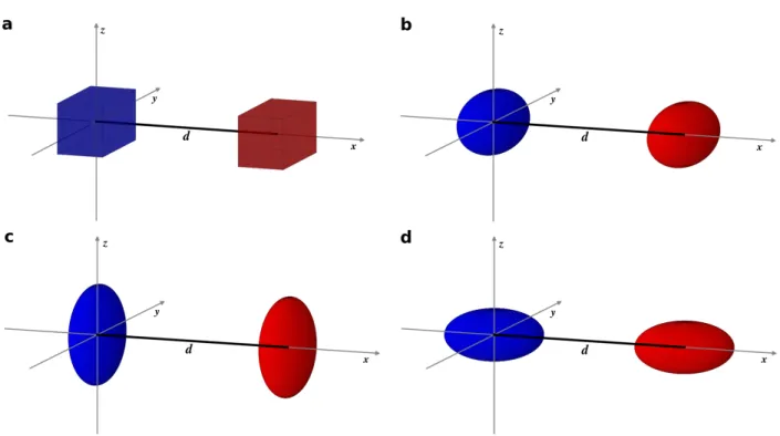
• 10.1.1 (1 point) Imagine two solid, oppositely and homogeneously charged prolate (i.e., elon- gated) ellipsoids with no external forces other than friction acting on them. Due to their opposite charges, they will attract each other. If we assume that the two bodies cannot ex- change charge, how will they eventually align (tip-to-tip, side-by-side, etc.)? Give reasons for your answer.

In Gaussian units (ε = 1), the electrostatic interaction energy of two homogeneously charged bodies with volumes V ₁ and V ₂ , and total charge +1 and −1, respectively, is given as

E = − Z

V

Z

V

1

|~ r 1 − ~ r 2 | d~ r ₁ ~ r ₂ (1) In the remainder of this task, you will estimate this distance-dependent interaction energy between different oppositely, homogeneously charged objects by means of Monte Carlo integration.

• 10.1.2 (1 point) Implement a Python function cuboid(n, dimensions) which returns an n × 3 array containing n random points that are uniformly distributed within a cuboid (German:

“Quader”) with edge lengths 2R _x , 2R _y , 2R _z and its center at the origin. The parameter dimensions is assumed to be a NumPy array containing the values of R x , R y , and R z .

1

Hint Uniformly distributed random numbers can be generated with the command numpy.random.uniform() . Read the corresponding Numpy documentation before use!

• 10.1.3 (2 points) Implement a Python function ellipsoid(n, dimensions) which returns an n × 3 array containing n random points that are uniformly distributed within an ellipsoid with principal half-axes of length R x , R y , R z and its center at the origin. The parameter dimensions is assumed to be a NumPy array containing the values of R _x , R _y , and R _z .

Hints

– The surface of an origin-centered ellipsoid with principal half-axes of length R x , R y , R z is the set of all points ~ r :=





 r _x r _y r z





 for which _R ^r

x

2

+ _R ^r

y

2

+ _R ^r

z

2

= 1.

– The easiest approach to generate uniformly distributed random points within a non- rectangular shape is to generate such points within a rectangular bounding box and dis- card all points that lie outside the shape. Note, however, that this method becomes very inefficient for more than three dimensions!

– A very useful function for this task is numpy.where() .

• 10.1.4 (3 points) Implement a Python function compute_energy(d, n, shape, dimensions) which uses Monte Carlo integration to estimate the electrostatic interaction energy between two oppositely, homogeneously charged objects according to Eq. (1). The parameter d is one of the objects’ displacement in x-direction. The parameter shape is used to pass the function that generates the support points, i.e. either of the previously implemented functions cuboid or ellipsoid .

• 10.1.5 (3 points) Now, the function compute_energy() shall be used to estimate the electrostatic interaction energy between objects of the following shapes:

– two cubes (R _x = R _y = R _z ) – two spheres (R x = R y = R z )

– two side-by-side prolate ellipsoids with R _x = R _y = ^R ₂

– two tip-to-tip prolate ellipsoids with ^R ₂

= R y = R z

In all cases, the volumes of the objects shall be V ₁ = V ₂ = 1. The different combinations are also sketched in Fig. 1.

For each combination, estimate the interaction energy for 20 separations d distributed on the interval (2R x , 5] (note the half-open interval!) using n = 10000 samples per separation. Plot the obtained energy versus distance together with the solution for two point charges.

Describe what you observe (e.g., similarities or differences between the curves). According to the plot, which is the energetically most favorable configuration? How does this correspond to the answer you have given in task 10.1.1?

Hint The volume of an ellipsoid with principal half-axes of length R _x , R _y , R _z is V = ^4π ₃ R _x R _y R _z .

2

Figure 1: Different scenarios to consider. The distance d between the centers is indicated by a thick black line.

a: Two cubes. b: Two spheres. c: Two prolate ellipsoids in a side-by-side arrangement.

d: Two prolate ellipsoids in a tip-to-tip arrangement.

3