Verbesserte Tuningmethoden von Monte Carlo Generatoren
Improved tuning methods for Monte Carlo generators
Abschlussarbeit im Masterstudiengang Physik von Fabian Klimpel
am Max-Planck-Institut für Physik
Erstgutachter: PD Dr. Stefan Kluth
06. September 2017
MPP-2017-281
Fabian Klimpel
München, den 06. September 2017
Contents
1 Introduction . . . . 1
2 The Standard Model of Particle Physics . . . . 3
2.1 Elementary particles . . . . 3
2.2 The evolution from initial state to nal state hadrons . . . . 10
3 Parameter-based tuning approach using the Professor framework . . . 23
3.1 Tuning approach . . . . 23
3.2 Applying a parameter tuning based on a previously performed tune . 32 3.3 Minimization without limits of parameter values . . . . 36
4 Bayesian Analysis Toolkit . . . . 39
4.1 Bayesian analysis . . . . 39
4.2 Working principle of BAT . . . . 46
4.3 Results . . . . 51
5 Adaptive polynomial interpolation . . . . 58
5.1 Mathematical model . . . . 59
5.2 Results . . . . 65
5.3 Comparison between Minuit and BAT . . . . 78
5.4 Uncertainty calculations using covariance matrices . . . . 80
6 Summary and conclusions . . . . 89
A Tuning setup . . . . 91
A.1 Pythia 8 conguration . . . . 91
A.2 Rivet analyzes . . . . 93
A.3 Observables and weights . . . . 96
B Professor based tuning . . . 102
B.1 Distribution of the run-combinations . . . 103
B.2 Distribution of the run-combinations without parameter ranges . . . . 109
C Minimization using BAT . . . 115
C.1 Program structure and Implementation . . . 115
C.2 Marginalized posterior pdfs . . . 120
C.3 Re-run . . . 122
D Algorithmic implementation of the adaptive interpolation . . . 124
D.1 Implementation structure . . . 124
D.2 Implementation of the for-loop . . . 127
E Distribution of the run-combinations with adaptive interpolation . . . . 129
F Tuning the adaptive interpolation with BAT . . . 133
F.1 Default set of observables . . . 133
F.2 Modied set of observables . . . 135
Bibliography . . . 137
Chapter 1 Introduction
The general purpose of particle physics is the identication of elementary particles, the measurement of their properties and the interactions between them. This led to the construction of the standard model of particle physics (SM) [1, p. 46]. This model is a theoretical construction that was created in agreement with experimental data and generated predictions for further measurements. The general interaction between theory and experiment is displayed in Fig. 1.1.
Theory
Predictions / Hypotheses Observation
Experimental data
design and perform an experiment analyze and
interpret
compare derive
Figure 1.1: Illustration of the interaction between theory and experiment. This graphic is based on a graph from Ref. [2].
The data analyzed in high-energy physics is mainly produced in collider experi-
ments. In such a setup, it is possible to collect data from a controllable environment
that allows precise measurements. Also, these experiments are (theoretically) re-
peatable. This is important due to the fact that the interactions in particle physics
are not deterministic and the measurements cannot be performed with innite accur-
acy. If a process under study has a large production cross-section and/or the collider has a large interaction rate, the statistical uncertainty on the measurements can be strongly reduced which allows to derive meaningful results.
Another problem in collider experiments arises from the setup itself. The initial state is the particle beam itself. Its properties like energy distribution or the spatial particle distribution in a bunch can be measured before the actual series of meas- urements start. The precision and accuracy of a detector can also be determined beforehand. The detector allows a collection of nal state information. But both of these measurements carry a certain uncertainty or can only be modeled. This underlines the importance of repeatable measurements. Additionally, the processes that happen between the particle collision and the signal in the detector remain at most indirectly measured. The collection of all those information of a single particle collision is called an event.
In order to describe the properties and interactions of elementary particles, a theoretical description is needed. These predictions are e.g. indirect limits on the masses based on experimental data. Also data were interpreted afterwards as the discovery of new elementary particles like the strange quark [1, p. 28].
The theoretical description which is used today is the SM. Although the SM is a very successful theory for data description, several extensions exist which predict new particles (e.g. the Minimal Supersymmetric Standard Model (MSSM) [3]).
The particles in the SM as well as their interactions will be described in the rst part of Chapter 2.
Theoretical models are used to describe the transition between the initial collision and the nal state measurement in a particle collider. The probabilistic models used for that description will be presented in the second part of Chapter 2.
These models are part of Monte Carlo (MC) simulation frameworks like Pythia 8 [4, 5]. The goal of such a simulation is to reproduce the actual meas- urements and serve therefore as the link between theory and experiment. For that purpose, model parameters need to be set in order to give a good data description.
A procedure for the model parameter estimation will be described and performed
in Chapter 3. A detailed investigation of several parts that will be mentioned there
will be discussed and analyzed in the Chapters 4 and 5. The investigation of the
tuning procedure will be summarized in the Chapter 6.
Chapter 2
The Standard Model of Particle Physics
In this Chapter, the elementary particles in the SM and the interactions between them will be introduced. At rst, the leptons and quarks will be introduced together with their most important properties. Secondly, the interaction between the particles of the SM will be presented. In the second part of this Chapter, the working principles of Monte Carlo (MC) generators will be discussed.
2.1 Elementary particles
This Section is meant take a closer look at the question which elementary particles in the standard model of particle physics (SM) exist. After a short overview over the fermions in the rst part of Subsection 2.1.1, the possible interactions will be presented in the Subsection 2.1.2. The content of the short overview of particle properties is mainly extracted from Ref. [1].
2.1.1 The standard model of particle physics
The SM is meant to describe the constituents of all matter. Additionally its goal is to describe the interaction between those constituents. The elementary particles exist either with a half-integer or a integer spin. Half-integer spins are called fermions and exist in the SM as leptons and quarks. Interactions are mediated by particles with integer spin, called bosons. Up to date, six leptons and six quarks are known.
These leptons are split in three generations. Each of those generations contains two quarks, one charged and one neutral lepton. Those parts will be explained further in the following.
For leptons, the rst generation contains the electron
eand the electron neutrino
νe. Beside their dierent electric charge
q, their masses are also signicantly dier-
ent. To distinguish the particles of this generation from the other two, beside the
dierences in their mass three further characterization numbers were introduced:
electron number
Le, muon number
Lµand tau number
Lτ. Furthermore, in every generation there is always a charged particle (electron
e, muon µ, tau τ) and a neutral particle (electron neutrino
νe, muon neutrino
νµ, tau neutrino
ντ). Their characteristic numbers are shown in Table 2.1. Additionally, every lepton has a weak isospin
T. For left-handed particles (cf. [6, p. 46]), a lepton generationforms a doublet state. The charged particle always has a third component of
Tz = −1/2and the respective neutrino has the component
Tz = 1/2[6, p. 299].
For the case of right-handed particles, the weak isospin forms a singlet state with a zero third component for the charged lepton, since neutrinos cannot be right-handed.
generation lepton
q [e] m [M eV] Le Lµ Lτ1
e-1 0.5109989461
±0.0000000031 1 0 0
1
νe0 < 0.460
·10−3(CL = 95%) 1 0 0
2
µ-1 105.6583745
±0.0000024 0 1 0
2
νµ0 < 0.19 (CL = 90%) 0 1 0
3
τ-1 1776.86
±0.12 0 0 1
3
ντ0 < 18.2 (CL = 95%) 0 0 1
Table 2.1: Overview of the leptons, their generations, charge
q, mass m, electronnumber
Le, muon number
Lµand tau number
Lτ. The masses are taken from Refs. [7,8].
Similar to the leptons, the quarks can also be characterized by their charge and mass inside a generation. Here, the dierence to the lepton numbers is the introduction of six avors. Those are called downness
D, upness
U, strangeness
S, charmness C, bottomness Band topness
T. Their properties are shown in Table 2.2. Quarks carry additionally a quantum number called color charge that is either red, green or blue. This charge is necessary in order to create an ad- ditional degree of freedom to describe the existence of hadrons that contain three quarks of the same avor. Otherwise, this would be forbidden by the Pauli-principle.
For the case of leptons and quarks, these were only half of the constituents. The
other half consists of their antiparticles. In that case, every characterization number
introduced above but the mass is inverted. For quarks, the color is also inverted and
referred to as anti-red etc. With respect to the antiparticles, the lepton numbers,
avors, colors are as the charge conserved in interactions.
2.1 Elementary particles
Generation Quark
q [e] m [M eV] D U S C B T1
d-1/3
4.8+0.5−0.3-1 0 0 0 0 0
1
u2/3
2.3+0.7−0.50 1 0 0 0 0
2
s-1/3
95±50 0 -1 0 0 0
2
c2/3
1275±250 0 0 1 0 0
3
b-1/3
4180±300 0 0 0 -1 0
3
t2/3
(173.21±0.51±0.71)·1030 0 0 0 0 1 Table 2.2: Overview over the quark, their generations, charge
q, mass
mand avor.
The masses are taken from Ref. [9].
2.1.2 Interactions
Now that the fermions are introduced, the goals will lie on the interaction between them in this Subsection. Interaction in particle physics means the exchange of particles in order to transfer energy, momentum etc. In the SM, one can distin- guish four dierent forces of interaction. The rst one is the electromagnetic force.
Its exchange particle is the photon
γ. This force aects every electrically charged particle.
The second force, the weak force, occurs due the electric neutral
Z0, the positively charged
W+and the negatively charged
W−boson. This force aects every fermion mentioned before. Also, interaction between those three bosons is possible.
The third force, the strong force, is driven by gluons
g. This kind of interaction isexclusively for quarks. In other words, the gluon only interacts with particles that carry a color charge. The gluon carries itself two color charges: a color and an anti- color. This construct leads to an overall of eight dierent gluons according to their color conguration. Since gluons carry a color charge themselves, they can interact with each other.
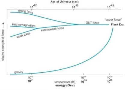
The last force is the gravitation, driven by the (hypothetical) graviton, but since this force is too weak, it is not considered in the SM yet. However it is a part in physics beyond the SM. Therefore, the gravity will not be mentioned further. The relative strengths of these forces are shown in Fig. 2.1. In the following those forces will be described in more detail.
2.1.2.1 Electromagnetic interaction
The electromagnetic interaction is the oldest theory and formally described by the
theory of quantum electrodynamics (QED). This interaction only aects electrically
charged particles. In such an interaction, particles exchange photons
γ. A graphical
representation of the exchange are Feynman diagrams (see Fig. 2.2). Important is
the feature, that an interaction can become arbitrary complicated due to the fact
Figure 2.1: Relative strength of the forces at certain energies/temperatures/ages of the universe. The graph is taken from Ref. [10].
that only the ingoing and outgoing particles underlie the particles boundary like the mass. In addition the ingoing and outgoing system needs to match in conservation of quantum numbers such as the avor, lepton number etc. Inside the interaction process, there can be many exchanges, inuencing the predicted results. Some ex- amples are shown in the lower row of Feynman diagrams in Fig. 2.2. The regulation for the number of vertices is given by the coupling constant
αEM = ¯hce2 ≈ 1371. Since
αEM < 1, the probability for a higher number of interactions
nis suppressed by
O(αnEM).2.1.2.2 Weak interaction
The weak force interacts with every quark and lepton as well as the mediators of the weak force. For a leptonic case, the process is only observed if the lepton numbers mentioned in the previous part are conserved additionally to the regular conservation laws like the energy, charge etc. For a neutral current interaction via the exchange of a
Z0boson, the participating ingoing and outgoing particles with respect to their conservation numbers underlie the same constraints like in the electromagnetic case.
With the charged current interaction mediated by the
W+and
W−bosons, the
weak force allows further interactions constrained to a charge of
±1e. This leads to
a larger number of possible interactions in the weak force than in the electrodynamic
2.1 Elementary particles
Figure 2.2: Feynman diagrams of electrodynamic interactions. The top one represents a simple interaction between two leptons. The four diagrams below show possible perturbations in the process.
case. Such processes in the leptonic cases are illustrated in Fig. 2.3.
The comparisons of the weak force to the electromagnetic were not chosen acci- dentally. As the Fig. 2.1 already implies, both forces can be formulated combined in the electroweak force (cf. Ref. [11]).
For the case of a charged weak interaction including quarks, the conservation of
avors is not directly fullled due to possible transformations like
d → u+W−.
Furthermore, the description of quarks in the context of weak interaction leads to
an understanding that every quark can be expressed as a superposition of quarks of
the same charges (including color). A numerical treatment of the probabilities that
a quark avor couples to another quark avor is given by the Cabibbo-Kobayashi-
Figure 2.3: Feynman diagrams of charged weak interactions of the processes
µνµ→νee(top) and
µ → νµνee(bottom). The additional charged current allows more possible in the weak interaction than the in electrodynamic interaction.
Maskawa-matrix (CKM-matrix):
Vud Vus Vub Vcd Vcs Vcb Vtd Vts Vtb
=
0.9705to 0.9770 0.21 to0.24 0. to0.014 0.21to 0.24 0.971to0.973 0.036to0.070
0. to0.024 0.036to0.069 0.997to0.999
(2.1) If the CKM-matrix would be a unitary matrix, then this would allow a conservation in the sum of the avors of a generation, e.g. upness + downness. This construction would be comparable to the leptonic numbers. But since this is not the case, decays as
Λ → p++π−or
Ω− → Λ +K−are possible. Beside pure partonic (between color-charged particles) or leptonic interaction, in a weak interaction, an exchange boson e.g. emitted by a quark can interact with a lepton as in the electromagnetic case. Even interactions between weak bosons are possible.
2.1.2.3 Strong interaction
The strong force is described by quantum chromodynamics (QCD). The exchange
particle is the gluon
g. This force only occurs between colored objects. Gluons carry
a color and an anti-color charge and are therefore able to change the color of a quark
but not its avor. Also, in strong interaction, the color is conserved. Due to the fact
that gluons carry those colors they are able to couple with other gluons. This results
in vertices with three and four gluons (cf. Fig. 2.4).
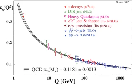
2.1 Elementary particles An important dierence between the electroweak and the strong force is the coup- ling constant. While
αEMcan be treated as almost a constant, the strong coupling
αsis not as shown in Fig. 2.1. Known as the asymptotic freedom, the coupling between the strong interacting particles strongly depends on their energy scale as shown in Fig. 2.5. An alternative graph could be drawn that shows the dependence of the coupling strength as a function of the distance between the quarks. The relation between energy scale
Qand distance
ris given by
Q(r) ∝ r−1. In that case, the asymptotic freedom would be reached at smaller distances, the coupling would be stronger at bigger distances. At large distances between particles, the asymptotic freedom leads under the connement to the creation of a quark-anti-quark-pair (
qq¯).
The connement states that colored particles cannot be isolated. Following that rule, hadrons are always color-neutral. This property needs to be fullled by the combination of all quarks + gluons (collectively called partons) in a hadron.
Figure 2.4: Feynman diagrams of vertices with three and four gluons.
2.1.2.4 Summary of the SM
As a summary, the main properties of the mediators are presented in Tab. 2.3.
mediator
m [eV] q [e]spin color charge
γ <10−18 <10−35
1 X
Z0 (91.1876±0.0021)·1090 1 X
W+ (80.385±0.015)·109
1 1 X
W− (80.385±0.015)·109
-1 1 X
g
<
O(M eV)0 1
√Table 2.3: Overview over masses
m, the electrical charges
q, the spin and the color charge of the mediators in the SM. The information is taken from Ref. [12].
Summing up all particles, this results in a total number of 12 (6 leptons + 6 anti-
leptons) + 36 ((6 quark + 6 anti-quarks)
·3 color charges) + 12 (1 electromagnetic
+ 3 weak + 8 strong mediators) + 1 (Higgs boson) = 61 particles that form the
SM. These are shown in the summary Fig. 2.6. Their interactions are summarized
in Fig. 2.7.
Figure 2.5: Dependence of the strong coupling constant
αsof the energy scale
Q.At higher
Qvalues, the coupling strength decreases further, so that in the limit a colored particle is asymptotically free. The picture is taken from Ref. [13].
2.2 The evolution from initial state to nal state hadrons
In the previous Section, the constituent particles of the SM were presented. In this Section, high energy physics (HEP) will be considered. The interactions will remain the same as before, but there are more particles and more possible processes to consider due to the high energy.
In order to handle those more complex systems, the evolution from an initial state, e.g. in
e+e−-collisions with xed center-of-mass energy
√s
, to observable hadrons, leptons and photons is divided in three parts. The rst one is the hard process. Here, the particle(s) of interest can be created together with additional partons e.g. in the process
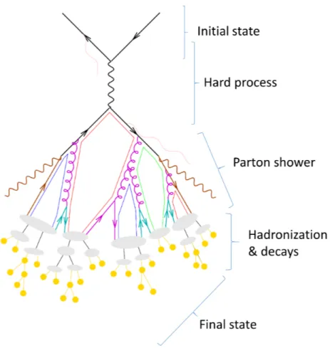
e+e− → Z0/γ∗ → qq¯. In the second step, the outgoing particles radiate further particles and thus create a so-called parton shower. During this period, their energy is reduced until the third stage is reached. This is the phase of hadronization. Since the average energy of the partons gets reduced due to the radiation, this phase treats the connement of the partons in contrast to the previous phase. At that point, hadrons are created, fragmented and decayed until they are registered in the detector. An overview over the evolution is shown in Fig. 2.8.
In reality, these phases are not distinguished but it is a simplication so that it
can be treated better in simulation programs, the so-called MC generators. Since it
2.2 The evolution from initial state to nal state hadrons
Figure 2.6: Summary of the particles of the SM without anti-particles. The quarks are shown in violet, the leptons in green, the bosons in blue and the Higgs boson in gray. Quarks and leptons are divided in generations column wise. Furthermore, the most important properties are displayed for every particle. The picture is taken from Ref. [14].
is the working principle of the generators, in the following the three phases will be described in chronological order in more detail. The content of this Section, if not stated otherwise, is extracted from Ref. [15].
2.2.1 Hard processes
The rst step is the calculation of the matrix element for the transition of the initial
state to the nal state that will be handed over to the following shower phase. This
calculation can be done at xed order in
αs. But since eects like self coupling gluons
and
qq¯-loops are possible inside e.g. a
pp-collision, the inner structure of a proton
would be needed to be known in order to be able to calculate a cross-section. At
that point the so called factorization theorem becomes important. This states for a
parton
iwith the momentum
piof a hadron with a momentum
phand the relation
pi = xiphthe separation of the parton density function (PDF)
ffrom the actual
Figure 2.7: Overview over the particles in the SM as the black dots. The blue lines represent the possible interactions between the constituents. The graph is taken from Ref. [16].
cross-section
σof the process in a calculation. For a lepton-hadron-collision, this delivers the form
σlh =X
i 1
Z
0
dxi
Z
dΦffi,h(xi, µ2F)dˆσli→f(xi,Φf, µ2F)
dxidΦf
(2.2)
for a cross-section
σlh. The variable
iruns over all incoming partons,
fstates the number of nal state partons.Φ
frepresents the Lorentz-invariant phase space, the PDF is represented by
fi,h,
σˆli→fis the partonic cross-section for the actual process of an interaction of a lepton
land the parton
ito form a nal state with
fpartons.
µFis the factorization scale and serves as dividing term between the PDF and the partonic cross-section term. While the PDF needs to be measured,
dˆσcan be calculated within perturbation theory. For hadron-hadron-collisions, this would deliver a similar form (cf. Ref. [15, p.20]).
Since measurements and particle properties are related to observables, the cross-
2.2 The evolution from initial state to nal state hadrons
Figure 2.8: Illustration of the evolution of an initial state before a particle collision to a nal state. The picture is taken from Ref. [17].
section for a certain observable will be considered. The according formula for the matrix element is given by
dσF
dO
matrix element
=
∞
X
k=0
Z
dΦF+k
| {z }
Plegs
∞
X
l=0
MF+k(l)
| {z }
Ploops
2
δ(O − O(ΦF+k))
(2.3)
for the dierential cross-section
dσdOF, a nal state
Fand an observable
O. The
amplitude for the production of
Ftogether with
kadditional partons, so called legs,
and
ladditional loops is denoted as
MF(l)+k. The integration is performed over the
k l
perturbative order and amount of jets
0 0 LO for F production
n 0 LO for F+ n jets
k+l≤n
N
nLO for F,N
n−1LO for F+1 jet ...
Table 2.4: Name giving scheme for a number of legs and loops. The former increases the number of outgoing jets, the latter the order of calculation.
Figure 2.9: Coecients used for a perturbative calculation in LO. The left picture shows the production of
Fnal state partons, the right
F + 2partons. The half shaded box implies the restriction, that exactly two jets are resolved. In other words, this implies the need for a phase-space cut.
phase space
ΦF+k. The
δ-function leads to the evaluation of Oon the momentum conguration
ΦF+k. This is denoted
O(ΦF+k)[15, p. 24].
The variables
kand
lcan be used for order classication as shown in Tab. 2.4.
Limiting the nested sums in Eq. 2.3 leads to a xed-order truncated calculation in the perturbative QCD (pQCD). Applying pQCD is a legitimate tool for this problem, since
αsis considered small (e.g.
αs(MZ) = 0.1181(11)[18]) in the hard process.
The problem arising from a simple integration of Eq. 2.3 over the phase space
dΦF+k, is the so called infrared divergence due to up to
kcollinear or soft partons.
Hence, these must be regulated by cuts in the angles, energies etc. The cut is set in a way, that the relation
σk+1 σkholds [15, p. 25]. This allows the truncation of Eq. 2.3.
In practice, the divergences are restrained by the KLN theorem [19, 20] using
multiple matrix elements that cancel divergent parts out. Those parts can be used
in the pQCD regime. While in leading order (
l= 0), the case
n= 0, that represents
the Born-level cross-section, can be handled without further problems, more legs
need a phase space cut to remain nite. This cut is meant to the phase space with
exactly
kresolved jets. This is illustrated in Fig. 2.9.
2.2 The evolution from initial state to nal state hadrons
Figure 2.10: Terms used for a perturbative calculation in NLO. The left picture shows the production of
Fnal state partons, the right
F + 1partons. The half shaded box implies the restriction, that exactly one jets are resolved. In other words, this implies the need for a phase-space cut.
Going to the next-to-leading order (NLO,
l= 1), the respective element is not nite anymore. In order to handle this, more matrix elements are used (see Fig. 2.10). This leads to the formula
σN LO0 = Z
dΦ0|M0(0)|2 + Z
dΦ1|M1(0)|2 + Z
dΦ02Reh
M0(1)M0(0)∗i
(2.4)
=σ0(0) +σ(0)1 +σ0(1)
(2.5)
with
σ(l)k. The divergence of the second and third term will cancel out, while the Born-level cross-section is nite. If
k6= 0, the cut mentioned above concerning theexact number of
kresolved jets still needs to be performed. Going further to next-to- next-to-leading order (NNLO), further matrix elements need to be taken into account in a cascade manner down to LO matrix elements. Since the relation
σk+1 σkneeds to be fullled by the phase-space cuts, the parts with
k+ 1are only corrections in pQCD.
2.2.2 Parton showers
In this part, the evolution of the particles from the high energy nal state of the hard
process to a hadronic state will be presented. For the evaluation of a shower evolution
one still needs to keep the restriction to small
αsvalues and to the relation
σk+1σk.
This needs to be used in order to control soft/collinear divergences in the shower
evolution. Furthermore, the shower leads to a reduction of the energy of the particles
while radiating further particles. So the algorithm needs to hold from a high energy
regime down to the hadronic scale, where increasing
αsvalues lead to breakdown of
pQCD. In order to handle this problem, one can start with reconsidering at Eq. 2.2.
The PDF
fi,hincludes so-called resummations of perturbative corrections to all orders from the initial scale of order of the mass of the proton, up to the factorization scale,
µF[15, p. 35]. In order to calculate the dierential cross-section as in Eq. 2.3 one needs to take a look at the xed-order calculations in
dˆσij→f. These calculations need to be concerned from the QCD up to the factorization scale. This will be performed in two steps. First of all an innite amount of legs will be treated. In a second part, an innite amount of loops will be considered. Using a combination will lead to a possibility to calculate the cross-section for
F+kjets.
2.2.2.1 Innite number of legs
In order to calculate the cross-section for an innite amount of legs, a possible ap- proach relies on resummation techniques. Such an approach can start with consid- ering two color-connected partons
Jand
Kin the state
F. The squared amplitude of the emission of a parton is given by
|MF+1|2=gs2NC
2sik sijsjk
+
collinear terms
| {z }
≡AntennaF unction
|MF|2
(2.6)
with
g2s = 4παs, the color factor
NCand
sijthe invariant between parton
iand
j. The indices
iand
krepresent the partons after the emission of
j. With respect to the parameter
sij, the possible infrared (IR) divergences in the soft or collinear limit can be extracted. The denition of this parameter delivers for massless partons the relation
sij ≡2pipj
(2.7)
= (pi+pj)2−m2i −m2j
(2.8)
= 2|pi||pj|(1−cos(θ))
(2.9)
= 2EiEj(1−cos(θ))
(2.10)
with the angle
θbetween
iand
j. In the soft limit (|pj| → 0) sij → 0. Thesame result would be in the case of
θ→ 0. This formulation becomes more visible in another calculation. The parameters
sijand
sjkare directly linked to the phase- space by the four-vectors, such that a connection between those can be formulated.
This proceeds by calculating the dierential of Eq. 2.10:
dsij sij
dsjk sjk
∝ dEj Ej
dθij θij
+dEj Ej
dθjk
θjk
(2.11)
2.2 The evolution from initial state to nal state hadrons
Figure 2.11: Visualization of the branching
qq¯→ qg¯qfor dierent values of
sijand
sjk.
Both cases would produce a singularity in the amplitude due to
1/Ej,
1/θijor
1/θjkterm. Besides the better visibility of the singularities, Eq. 2.11 shows the reason for the names soft and collinear. This is graphically shown in Fig. 2.11.
Therefore this must be constrained in order to use Eq. 2.6 as the amplitude for the calculation of Eq. 2.3 since the integration is performed over the whole phase-space.
For that purpose, a cuto parameter
µ2IRwill be used as a minimum scale. This parameter is also called minimum perturbative cuto scale.
The Eq. 2.11 additionallly allows an ordering of the shower. A collection of typically used ordering parameters are shown in Fig. 2.12. Which ordering is used depends on the MC generator. During the shower evolution, the algorithm will integrate over the whole ordering parameter over and over again. The choice of the ordering parameter empowers or weakens certain radiations. This aects the virtual corrections via the so-called Sudakov factor [21]. In the end, Eq. 2.6 delivers a powerful recursion formula that is able to calculate a parton shower with arbitrarily many particles until the hadronization. Note that all those calculations are only performed in leading order.
The recursion formula of the amplitude
|MF+n|2needs to be integrated over the (cut) phase-space in order to get the respective cross-section as shown in Eq. 2.5.
Performing this calculation delivers a result with the algebraic structure
σF0+n=αns(ln2n+ ln2n−1+ ln2n−2+...+ ln +F)
(2.12)
Figure 2.12: An overview over the most common shower evolution parameters used in MC generators. Variants of the dipole approach are implemented in ARIADNE, SHERPA and VINCIA. Angular ordering is used by HERWIG 7. The
pTordering is implemented in PYTHIA 6 and 8. The rightmost represents the evolution of only one parent.
with the form
lnλthat denotes a transcendentality
λ. The function
Fdenotes a rational function with
λ= 0. This series is usually cut at a certain term in order to speed up the computation. The easiest cut includes only the
ln2nterm and is called the double logarithmic approximation (DLA). Including additionally the
ln2n−1term is called the leading-logarithmic (LL). In order to improve the calculations with the underlying series cut, further calculations are performed such as explicit momentum conservation, gluon polarization and other spin-correlation eects, higher-order co- herence eects, renormalization scale choices, nite-width eects, etc [15, p. 39].
Using more terms are called next-to-leading-log (NLL) etc. One needs to keep in mind that all those are approximations of the real solution and that a scale cut at
µIRstill needs to be performed. In order to get rid of the scale cut, a similar ap- proach as done in this Subsection will be performed but for innite loops in the next Subsection.
2.2.2.2 Innite number of loops
The underlying idea of this Subsection is the same as in the KLN theorem for the NLO calculation. With the goal of an integration over the full phase-space, the terms with
l >0will be taken into account such that the singularities will cancel out. For a
l= 1correction, this results in a contribution in the form of
2Reh
MF(0)MF(1)∗i
⊃ −gs2NC|MF(0)|2
Z dsijdsjk 16π2sijk
2sik sijsjk
+
less singular terms
.
(2.13)
The right-hand side is equivalent to the term of
σ(1)in Eq. 2.5. This expression is
2.2 The evolution from initial state to nal state hadrons
Figure 2.13: Coecients used for LO+LL approximation in the parton shower. The green box indicates that no approximation is needed for the calculation. In contrast, the yellow boxes indicate a LL approximation. The lled boxes show an integration over the whole phase-space without the need of scale cuts / IR divergencies. In the half lled boxes, the cuts are needed. The left picture shows the innite legs used in LO only, the right shows a KLN theorem like approach for the calculation of a
F+nnal state including innite loops.
a part of the term
2Re hMF(0)MF(1)∗
i
. Eq. 2.13 cancels the singularity from Eq. 2.6.
But since the calculation was performed for a series of leading-order terms for a
F+nparton shower and each term contains the singularities that need to be cut, that type of correction needs to be performed for every term. This is the actual resummation calculation. In a graphical illustration corresponding to Fig. 2.9, this can be shown as in Fig. 2.13. While the recursion of Eq. 2.6 implies a horizontal walk over a xed
lvalue, the Eq. 2.13 represents a diagonal movement along a xed
n=k+l. 2.2.3 Hadronization and fragmentation
During the parton shower, the energy of the partons is reduced due to further ra- diated partons. Therefore, the next phase treats the connement of the partons.
During that phase, the partons will build color-neutral hadrons. Those hadrons will further decay until a collection of stable hadrons is reached. In MC generators, the fragmentation of hadrons is described by a model.
A famous model for hadron fragmentation is called Lund-string-model. This model is implemented in the Pythia MC generator. In the following section, the main parts of the model will be described.
The Lund-string-model describes the hadronization and fragmentation. This
model simplies the hadronization by connecting partons in the same phase space
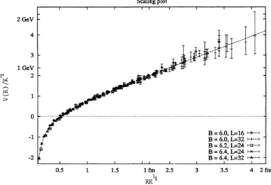
Figure 2.14: Potential of a
qq¯-pair as function of the distance between the quarks.
The picture is taken from [22].
via strings. In order to describe the fragmentation, these strings are allowed to break. A breaking string creates a new
qq¯-pair.
Firstly, two partons will be considered that are connected by a string. If both partons will be moved further apart, the string tension will rise. Analogously to classical mechanics, a potential
Vcan be formulated as
V(R) =κR
(2.14)
with the distance
Rbetween the partons and the string tension
κ. As the value of
κ, one can use values around
0.9 GeV /f m. If on the other hand the partons will be moved closer together, one needs to take Coulomb interactions with a
1/Rdependency into account. The superposition of these two potentials is shown in Fig. 2.14 for a
qq¯-pair. In fact, the Coulomb part is neglected in the model itself.
As the potential rises for bigger distances between the partons, the string breaks at a certain point. In the string breaking process, a new
qq¯-pair will be created as shown on the left-hand side in Fig. 2.15. If the distance between both partons of a newly produced hadron will also increase, the breaking will be repeated. This is shown on the right-hand side in Fig. 2.15.
Since the model does not provide an individual handling of the string breaking from
rst principles, the model explains the phenomenological treatment by a quantum
tunneling. The creation of a
qq¯-pair is connected with a certain transverse momentum
2.2 The evolution from initial state to nal state hadrons
Figure 2.15: Time dependent evolution of a
qq¯production during a string breaking (left). The right graph shows the evolution over a longer time period including further fragmentations. The right picture is taken from Ref. [23].
pT
for both partons. Here, the transverse direction is dened as the direction of the original string. The probability density for the actual
pT-value of the partons is in a gaussian shape of the form
P(m2q, p2T q)∝exp −πm2q κ
!
−πp2T q κ
!
(2.15) with the parton mass
mq. Note, that this is the transverse momentum for a single parton created in the string breaking. The second parton will get the negative value of the rst one's transverse momentum. Furthermore, the actual value of the
pTis avor independent because of the factorization of the mass and
pTand allows therefore a universal treatment of the string breaking in this model. The masses of the resulting hadrons after a string break are given by Breit-Wigner distributions.
An additional parameter that can be derived from this equation is the width of the gaussian functions given by
V ar[pT q] =E[p2T q]−E[pT q]2
(2.16)
=E[p2T q]
(2.17)
=κ/π≈(240M eV)2
(2.18)
with the mean
Eof a distribution and the respective variance
V ar, later referred as
σ2.
Another important aspect of the Lund-string-model is the fragmentation function parametrization, called the Lund symmetric fragmentation function,
f(z)∝ 1
z(1−z)aexp
−b(m2h+p2T h) z
(2.19)
with the free parameters
aand
band the fragmentation variable
z, e.g.
z= (E+pz)/(E+pz)total
[23, p. 6]. The mass
mhand the transverse momentum
pT hrefer to the hadrons produced in the fragmenting string.
One important aspect of the Lund-string-model is the handling of baryons. Until now, only strings between two partons were considered. In the case of three partons, the model will be expanded by a diquark, an object that is made out of two quarks.
In that case, the string connects a quark with a diquark. Using this construction,
the formalism mentioned before almost stays the same. In the case of the fragment-
ation function, the parameter
awill be modied by the addition of the parameter
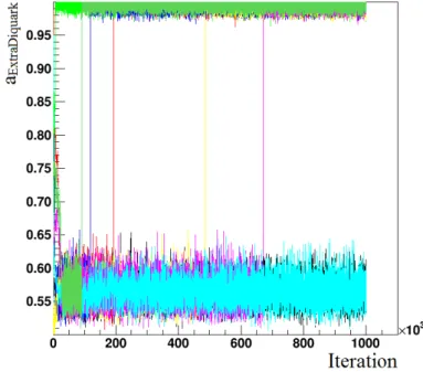
aExtraDiquarkin order to handle dierences between mesons and baryons [24].
Chapter 3
Parameter-based tuning approach using the Professor framework
For measurements and searches in high energy physics experiments, good simulations of the underlying physics processes are of utmost importance. For that purpose, so- called Monte Carlo generators are used. These MC generators are used to make predictions of physics processes. The calculations performed by the MC generators are model based. However, the models depend on parameters which cannot be derived from rst principles.
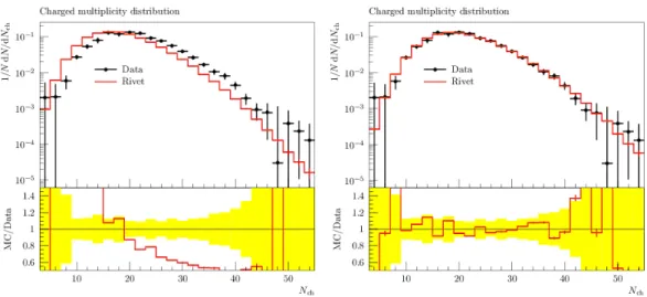
To illustrate the dependence of MC generator predictions on the parameters, an example is shown in Fig. 3.1. This Figure shows a comparison of the charged particle multiplicity distribution of the process
e+e−→Z0→qq¯at a center-of-mass energy
√s = 91.2 GeV
between the measurements performed by the ALEPH experiment [25] and a MC simulation using two dierent parameter sets. By visual inspection the graph on Fig. 3.1 (right) shows a better agreement of the MC prediction with the data compared to the graph on Fig. 3.1 (left). The goal is to estimate the parameter conguration for the simulation such that the MC generator prediction ts the data best. The search procedure for those parameter values is called tuning and has to be performed in a well dened way.
In this chapter, a tuning procedure will be described. This method is implemented in the Professor framework [26]. Beside explaining the tuning method in Sec. 3.1, the explicit implementation of such a tuning using Professor will be presented.
For that purpose, the reproduction of a previously performed tuning from Ref. [27]
will be described in Sec. 3.2. As a last step, the tuning will be re-performed with a modied setup in Sec. 3.3.
3.1 Tuning approach
Several dierent tuning approaches are available and used in HEP. In general, these
approaches can be separated into three dierent types [26]. The rst type mentioned
here is the manual tuning. This approach is in general done by hand and requires an
Figure 3.1: Illustration of the charged multiplicity distribution of a hadronic
Z0decay in an
e+e−collision with a center of mass energy of
√s=m(Z0) = 91.2 GeV
. The black dots are the measurements performed by the ALEPH collaboration [28] and provided by the Rivet framework [29], the red line is simulated with Pythia 8 [4,5]
based on two dierent sets of input parameters (cf. Tab. B.1).
appropriate expertise. The tuning can become complex for a more comprehensive parameter set.
The second type is called brute force tuning. Approaches in this category are constructed as a direct search. A direct search can be dened as a Markov Chain (MC), meaning the evaluation of the
n-th step determines the
(n+1)-th step through the parameter space. Such a point lies around the current point. An algorithm will then test the goodness of the proposal point and decide whether to change to that point or to stay at the current position. The benet of such an approach is a minimum of needed assumptions in order to nd a best parameter set in order to describe the measurements. On the other hand in this approach the MC generator needs to run for every new step resulting possibly in larger run-times. This can become especially complicated for more complex problems.
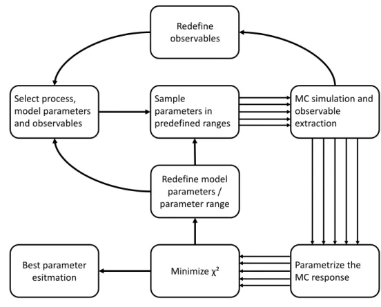
The third tuning type is the parametrization-based tuning. This approach is the one that is used in this thesis. The basic idea of the model parameter estimation is the calculation of a function which describes the MC generator response depending on the model parameters that need to be tuned. Using this function, the parameters are chosen such that the description of the data by the MC predictions is optimal.
For the purpose of calculating the needed function, many dierent congurations of
model parameters are used and a function of the associated MC generator response
is calculated. Since many congurations and therefore many simulations are needed,
3.1 Tuning approach
Select process, model parameters and observables
Sample parameters in predefined ranges
MC simulation and observable
extraction
Parametrize the MC response Minimizeχ²
Redefine observables
Redefine model parameters / parameter range
Best parameter esitmation
Figure 3.2: Procedure of a parametrization based MC generator tuning.
the calculation of such a response function is computing intensive. These calculations were complicated to realize formerly but are easier/possible nowadays (cf. Moore's law [30]).
An overview over the needed steps for this tuning approach is shown in Fig. 3.2.
Before a tune can be performed, the
nparameters of the MC generator that need to be tuned need to be specied. Secondly, each parameter needs a specic range.
Those are restricted either by the meaningfulness in the context of physics or at least limited by the developers of the MC generator framework itself.
In order to tune those parameters, observables and corresponding reference data are needed. The choice of the observables depends upon the parameters chosen.
The most important property in order to select them is the sensitivity. This term
describes the dependency of the value of an observable on the parameter value. A
further selection of the observables depends on the MC generator and the predic-
tion possibilities, e.g. whether it works in LO or NLO etc. After the selection is
performed, the reference data are provided by the Rivet [29] framework.
The rst tuning step consists of sampling randomized values for each parameter in its range. Thus, the results are
mparameter vectors
piwith
i ∈ [1, m]and
dim(pi) =n. The set of all those vectors will be called
S ={pi}i=1,..,m.
In the second tuning step, those vectors are used as the conguration of the MC generator. Every single conguration produces an output le containing all processes and properties of the particles in every simulated event. Such an output le can have a size of
O(GB) per 100,000 events. The large amount of storage can limit the number of events calculated in a single conguration or the number of congurations
m.In the third tuning step, a collection of observables from one or several experiments can be extracted for every conguration out of the simulated events. The calculated observables from the simulations allow a direct comparison with the reference data.
Using only the sampled parameter sets for a comparison would provide the best sampled parameter vector but this vector does not have to be the best possible parameter vector.
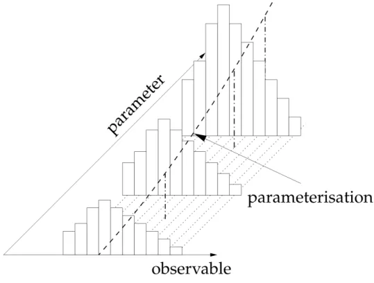
To avoid this, the MC response will be parametrized in the fourth step. The assumption that the variation per data point is suciently smooth while changing the parameter values (shown in Fig. 3.3) leads to the possibility of an interpolation approach between all sampled parameter sets with a smooth function. Furthermore, for the approach used in this thesis, all data points will be tted individually. In this way, the total number of obtained interpolation functions is equal to the total number of data points.
In order to get a good description by a function of the MC response inside the parameter space, the sample-density needs to be suciently high. Under the as- sumption such a sucient amount of sample points
min one dimension and within a given parameter range exists, a
n-dimensional tuning process would need
O(mn)samples. Therefore the number of samples with respect to the memory consumption and computing power needed in order to receive such an parametrization of the MC response is limited in terms of
n. This leads to a limitation of the model parameters that can be optimized in this tuning process.
In the last step, all interpolation functions should be optimized simultaneously in order to nd the smallest dierence between the functions and the measurements and thus the best
pfor reproduction of the measurements using the MC simulation.
For the purpose of sampling the anchor points
pias well as for parametrization and
minimization, the Professor 2.1.4 framework will be used. The working principle
of the framework will be described in the Subsection 3.1.1. The MC simulation
is provided by the Pythia 8 [4, 5] framework. The output le of Pythia 8 is a
complete record of all events. This output is used as the input for the Rivet 2.4.2
framework. This framework extracts physical observables out of the output les from
MC generators. Furthermore, Rivet provides the measured data for comparison
3.1 Tuning approach
Figure 3.3: Illustration of the impact of parameter values on an observable. This leads to a parametrization of the data points that only depends on the parameter values themselves. The sketch is taken from Ref. [31].
with the MC generator response. Those two frameworks will be presented in the Subsection 3.1.2.
3.1.1 The Professor 2.1.4 framework
The Professor framework in general is used for systematic parametrization-based
tuning. For that purpose, the framework provides Python-scripts and C++-
classes. In the following, the most important scripts for the intended tuning will be
presented. Those will be described based on the chronological order as displayed in
Fig. 3.2. This will be only a brief overview over the possibilities that the framework
provides, but since the content in this thesis needs comparability, some congur-
ations need to remain unchanged and are therefore neither used in this thesis nor
presented here. Note that this description considers Professor in the version 2.1.4.
If not mentioned otherwise, the following explanations are based on Ref. [26] and the source code of Professor 2.1.4 [32] itself.
3.1.1.1 prof2-sample
This script serves as a generator of random vectors
pi. The sampling is based on the Python standard library random [33]. The pseudo-random sampling algorithm is based on Ref. [34] and it samples uniformly in a predened range. A benet of using Professor in the version 2.x is, that the prof2-sample script directly writes the sampled vectors into the conguration les for a MC generator. So, after sampling, the MC generator can be run directly with these conguration les.
3.1.1.2 prof2-ipol
This script is the heart of the Professor framework. The script calculates a t function in order to parametrize the MC response for the given set
S. Since it is assumed that the parameter changes yield a suciently slow and smooth change in the MC response
M Cbin a data point
b, the Professor framework calculates for that purpose a polynomial tting function
f(b)(p). The calculation will be performed for every data point
bindependently but with in the same xed and predened order. In the case of a polynomial function of second-order, this looks like
M Cb(p)≈f(b)(p) =α(b)0 +X
i
βi(b)p0i+X
i≤j
γij(b)p0ip0j
(3.1) with the t parameters
α(b)0,
βi(b)and
γij(b). The prime of the MC model parameters indicates the mapping
p0i= pi−pi,min
pi,max−pi,min
(3.2)
with the minimum (maximum) value
pi,min(
pi,max) in the dimension
iof all sampled parameters in
S. Hence, the parameters are mapped onto a [0,1]-interval.
This is performed for numerical stability, since now the t parameters are more likely to be of the same order. Furthermore, since this transformation is a bijective shift, the mapping mentioned in Eq. 3.2 is possible without changing the function behavior.
The number of t parameters needed for the interpolation depends on the order of the polynomial function
nand
dim(p) =P. A general formula for the number of parameters
Nn(P)is given by [26, p. 3]
Nn(P)= 1 +
n
X1 i!
i−1
Y(P +j).
(3.3)
3.1 Tuning approach
In order to calculate the t parameters, at least
(|S|=Nn(P))∧(pi 6= pj∀ i, j ∈ [1, Nn(P)])
(3.4) needs to be fullled. Further anchor points provide additional information about the dependency on the parameters of the MC generator prediction. The authors of the framework recommend an oversampling of
|S| ≥2Nn(P).
For retrieving the t parameters, Eq. 3.1 can be generalized to arbitrary dimension and order, leading to
M Cb(p)≈f(b)(p) =
Nn(P)
X
i=1
c(b)i p˜i
(3.5)
with the t coecients
c(b)i. This vector
c(b)contains a dimension-wise combination of all t parameters like
α(b)0,
βi(b)and
γij(b)from Eq. 3.1. The vector
p˜of the
p˜iis called extended parameter vector. This vector contains every combination of every
picorresponding to the t parameter
c(b)i.
For a given set
Sand the corresponding set
{M C(b)}the tting problem from Eq. 3.5 can be formulated as
v(b)=P c˜ (b)
(3.6)
with the MC response vector
v(b), the matrix
P˜that row-wise consists of
p˜and the extended parameter vector
c(b). Explicitly, this can be written for a two dimensional polynomial function of second order as
v1 v2
...
v|S|
| {z }
v(values)
=
1 p01 p02 p021 p01p02 p022 1 p01 p02 p021 p01p02 p022
...
1 p01 p02 p021 p01p02 p022
| {z }
P˜(sampled parameter sets)
α0 βp0
1
βp0
2
γp0
1p01
γp0
1p02
γp0
2p02
| {z }
c(coe.)
.
(3.7)
With
|S| > Nn(P), this equation is overdetermined. The solution of the lin-
ear equation system delivers the t parameters for the polynomial function for a
given data point
b. The calculation of the solution is based on a singular value de-
composition (SVD). This algorithm decomposes the matrix
P˜of size
M ×Ninto
P˜ = U ·W ·VT[35, 36]. The matrix
Vis an orthonormal matrix of size
N ×N.
Uis a column-orthogonal matrix of size
M ×Nand
Wis a diagonal matrix with
Wii=wi
and size
N×N. Inverting this decomposition with respect to the problem in Eq. 3.6 yields
c(b)= ˜Ih P˜i
v(b)=V ·W−1·UTv(b)
(3.8) with the inverse operator
I˜[·]and the inverse
Wii= 1/wi. This method delivers the shortest
c(b). If
P˜is not invertible, the Roger-Penrose-Inverse [37] can be calculated.
That way, this method delivers in the invertible and non-invertible case the shortest length of
P c˜ (b)−v(b)[35].
In order to calculate the propagation of the uncertainty for the t parameters, which has its origin in the statistical uncertainty of the MC generated events due to the limited number of events, the framework provides several dierent options. The option that is used in this thesis is called symm inside the Professor framework.
This option is the closest to a t-parameter-by-t-parameter uncertainty estimation.
Here, the uncertainty calculation follows the same construction as in the t para- meter calculation, but the MC response values are exchanged by their corresponding uncertainties. Doing so, the correlation between the t parameters are neglected and the uncertainties of the t parameters will be overestimated.
3.1.1.3 prof2-tune
The third Python-script that will be used seeks the minimum of a goodness-of-t function
χ2. In the case of Professor, this function is given by
χ2(p) =X
O
X
b∈O
wb
(f(b)(p)− Rb)2
∆2b
(3.9)
with the weights
wbfor each data point
bof every observable
Oand the correspond- ing measurement
Rb. The squared uncertainty
∆2b = ∆2f+ ∆2Ris a combination of the uncertainty
∆2fof the t function
f(b)(p)and the uncertainty
∆2Rof the measure- ment
Rb. The weights can be chosen manually for each data point independently in order to provide a better MC response for some data points/observables, because the impact of a data point/observable becomes more important for the overall
χ2-value.
This function needs to be minimized which is done using the Minuit [38] package.
This package provides a gradient based method, called Migrad, which copes with high dimensional problems better than the SciPy Nelder-Mead simplex minimizer.
[26, p. 7]. In addition, the parameters can be calculated using parameter limits in order to stay in physical meaningful regions. Also, the resulting correlation matrix
ρij =Cij/pCiiCjj
![Figure 3.4: Measurement of a hadronic Z 0 decay performed by ALEPH [52]. The dierent colors represent the dierent layers of the detector](https://thumb-eu.123doks.com/thumbv2/1library_info/4004133.1540734/38.892.172.768.207.633/figure-measurement-hadronic-performed-dierent-represent-dierent-detector.webp)