for dimers H 2 -H 2 , H 2 -O 2 , F 2 -F 2 and H 2 -F 2 , and Monte Carlo simulations of the vapor-liquid

prediction of second virial coefficients

for dimers H ₂ -H ₂ , H ₂ -O ₂ , F ₂ -F ₂ and H ₂ -F ₂ , and Monte Carlo simulations of the vapor-liquid

equilibria for hydrogen and fluorine

Inaugural-Dissertation zur Erlangung des Doktorgrades der Mathematisch-Naturwissenschaftlichen Fakult¨ at

Universit¨ at zu K¨ oln

vorgelegt von Tat Pham Van

aus Vietnam K¨ oln, Germany

October 2006

Berichterstatter: Prof. Dr. U. K. Deiters

Institut f¨ ur Physikalische Chemie, Universit¨ at zu K¨ oln

PD. Dr. Thomas Kraska

Institut f¨ ur Physikalische Chemie, Universit¨ at zu K¨ oln

Tag der letzten m¨ undlichen Pr¨ ufung: 6.12.2006

This thesis has been carried out in Prof. U.K. Deiters’s group at the Institute of Physical Chemistry, University of Cologne.

I am taking this opportunity to thank all those who have assisted me in one way or the other with my Ph.D project.

Firstly I would like to thank my supervisor Prof. Ulrich K. Deiters. I thank him for giving me the opportunity to work in his group at University of Cologne. I have received his help since I started my PhD enrollment. During years in the Institute of Physical Chemistry I have known Prof Ulrich K. Deiters as a sympathetic person.

Secondly I am thankful to Priv.-Doz. Dr. Thomas Kraska who has given me a lot of important help. I am grateful to Dr. Nguyen Van Nhu for his special help over three years.

I also wish to thank Dr. L. Packschies (RRZK) for technical help with quantum mechanics calculations, furthermore Dr. P. K. Naicker, Dr. A. K. Sum (University of Delaware, USA), Dr. Zhu Yu (Nanjing University of Technology, China), Prof.

Dr. Anthony Stone (University Chemical Laboratory, United Kingdom) and Dr. J.

Karl Johnson (University of Pittsburgh, USA) for making available their computer programs. Especially I would like to thank Dr. Ronald Alle (Institute of Physical Chemistry, University of Cologne) who has given me much necessary help for my work.

I am grateful to all colleagues in our research group, for their help over three years, especially to Mr. Shirani, and to all members of the Institute of Physical Chemistry for their care and attention. I would like to acknowledge the work by Mr. Nguyen

i

Huu Hoa who gave me much help with correcting several computer programs. I got a lot of encouragement from Vietnamese students in Germany, especially from my friends in Aachen.

Furthermore I would like to thank the Government and the Ministry of Educa- tion and Training of Vietnam for the financial support over three years within the Vietnamese overseas scholarship program. I wish to thank the members of the steer- ing and the executive Committee for this overseas training project.

Finally, I am forever indebted to my parents, Mr. Pham Gia Trieu and Mrs. Ngo Thi Lua, my brothers, sisters, and especially to my wife, Pham Nu Ngoc Han, and my children, Pham Gia Huan and Pham Ngoc Gia Bao for their understanding, endless patience and encouragement.

K¨oln, September 2006 Tat Pham Van

Institute of Physical Chemistry University of Cologne

K¨oln, Germany

Die reinen Elemente Wasserstoff, Fluor und Sauerstoff sowie die Mischungen Wasser- stoff-Sauerstoff und Wasserstoff-Fluor besitzen zahlreiche industrielle Anwendungen.

Wasserstoff k¨onnte ein erneuerbarer Energietr¨ager bei Brennstoffzellen-Technologien werden und k¨onnte die anderen wichtigen Brennstoffe verdr¨angen. Daher ist die Berechnung der thermodynamischen Daten der oben genannten Systeme ein wichtiges Anliegen f¨ ur die praktische Anwendung.

Diese Arbeit enth¨alt die Ergebnisse der Berechnungen der vier Ab-initio-Paarpoten- tiale f¨ ur die Dimere H 2 -H 2 , H 2 -O 2 , F 2 -F 2 und H 2 -F 2 , der daraus abgeleiteten zweiten Virialkoeffizienten einschließlich der Quantenkorrekturen 1. Ordnung sowie der ther- modynamischen Phasengleichgewichtsdaten der Reinstoffe Wasserstoff und Fluor, wobei letztere mit der Gibbs-Ensemble-Monte-Carlo-Methode (GEMC) berechnet wurden.

Die neuen intermolekularen Wechselwirkungspotentiale der Dimere H 2 -H 2 , H 2 -O 2 , F 2 -F 2 und H 2 -F 2 wurden mit quantenmechanischen Methoden berechnet, und zwar mit Hilfe der Coupled-cluster-Theorie CCSD(T) und unter Verwendung korrelations- konsistenter Basiss¨atze aug-cc-pVm Z (m = 2, 3, 4); die Ergebnisse wurden zum Ba- sissatzlimit extrapoliert (hier mit aug-cc-pV23Z bezeichnet) und bez¨ uglich des “basis set superposition error” (BSSE) korrigiert. Die so erhaltene Potentialhyperfl¨ache f¨ ur das H 2 -H 2 -Dimer stimmt gut mit der von Diep und Johnson [25] vorgeschlagenen Hyperfl¨ache ¨ uberein. Zum Vergleich wurden auch st¨orungstheoretische Rechnungen mit der Møller–Plesset-Theorie zweiter und vierter Ordnung angestellt sowie Rech- nungen mit den Basiss¨atzen 6-31G und 6-311G, aber die Ergebnisse waren schlechter.

F¨ ur die Absch¨atzung der Genauigkeiten der theoretischen Methoden und der Ba- siss¨atze wurden verschiedene molekulare Parameter berechnet.

iii

Die quantenmechanischen Ergebnisse wurden f¨ ur die Erstellung von vier neuen ana- lytischen Paarpotential-Funktionen verwendet. Die anpassbaren Parameter dieser Funktionen wurden durch Anpassung an die Ab-initio-Wechselwirkungsenergien durch eine globale Minimierung der Fehlerquadrate bestimmt, und zwar durch eine Kom- bination des Levenberg-Marquardt-Verfahrens und eines genetischen Algorithmus.

Aus diesen Funktionen wurden die zweiten Virialkoeffizienten von Wasserstoff und Fluor sowie die Kreuz-Virialkoeffizienten der Systeme Wasserstoff–Sauerstoff und Wasserstoff–Fluor durch Integration ermittelt; dabei wurden Quantenkorrekturen ber¨ ucksichtigt. Die Ergebnisse stimmen mit experimentellen Daten—soweit vorhan- den—oder mit empirischen Korrelationen ¨ uberein.

Monte-Carlo-Simulationen unter Verwendung der Gibbs-Ensemble-Technik (GEMC) wurden eingesetzt, um mit Hilfe der analytischen Paarpotentiale den Dampfdruck von Wasserstoff und Fluor, die Dichten der koexistierenden fl¨ ussigen und gasf¨ormigen Phasen, die Verdampfungsenthalpie und -entropie im Temperaturbereich 18–32 K f¨ ur Wasserstoff und 60–140 K f¨ ur Fluor zu berechnen. Diese Temperaturintervalle reichen nahe an die kritischen Gebiete der Substanzen heran. Aus den berechneten orthobaren Dichten konnten die kritische Temperatur, der kritische Druck und das kritische Molvolumen abgesch¨atzt werden. Die Ergebnisse stimmen gut mit ex- perimentellen Daten sowie mit Berechnungen mit Hilfe von Zustandsgleichungen

¨

uberein. Ferner wurden zur Charakterisierung der Strukturen von Wasserstoff und

Fluor die Site-site-Paarkorrelationsfunktionen g(r) ermittelt.

The pure elements hydrogen, fluorine and oxygen and the mixtures hydrogen-oxygen and hydrogen-fluorine are used in several industrial applications nowadays. Hydro- gen might become a renewable energy carries in fuel cell technologies [122, 16].

Hydrogen is considered a fuel which can replace all the major fuels [46, 95]. Con- sequently, the estimation of thermodynamic data for the mentioned systems over a wide range of temperature and pressure is a need for future practical applications.

This thesis presents the results of the calculations of four new ab initio intermolecular pair potentials, the second virial coefficients with first-order quantum corrections of the dimers H 2 -H 2 , H 2 -O 2 , F 2 -F 2 and H 2 -F 2 , and thermodynamic properties of phase equilibria for the pure fluids hydrogen and fluorine derived from the Gibbs ensemble Monte-Carlo simulation techniques.

The new intermolecular interaction potentials of the dimers H 2 -H 2 , H 2 -O 2 , F 2 -F 2

and H 2 -F 2 were developed from quantum mechanics, using coupled-cluster theory CCSD(T) and correlation-consistent basis sets aug-cc-pVm Z (m = 2, 3, 4); the results were extrapolated to the complete basis set limit (denoted aug-cc-pV23Z).

The constructed potential energy surface of the dimer H 2 -H 2 turned out to be in good agreement with that proposed by Diep [25]. The interaction energies were cor- rected for the basis set superposition error (BSSE) with the counterpoise scheme.

For comparison also Møller-Plesset perturbation theory (at levels 2 to 4) as well as the basis sets 6-31G and 6-311G were investigated, but the results proved inferior.

Molecular properties were calculated for assessing the accuracy level of each the- oretical method and the basis set, respectively. The quantum mechanical results were used to establish four new analytical pair potential functions. The adjustable parameters of these functions were determined by global least square fits to the ab

v

initio interaction energy values by means of the Levenberg-Marquardt (LM) and the Genetic algorithm (GA). From these functions the second virial coefficients of hydrogen and fluorine as well as the cross virial coefficients of the systems hydrogen- oxygen and hydrogen-fluorine were obtained by integration; corrections for quantum effects were included. The results agree well with experimental data, if available, or with empirical correlations.

Gibbs ensemble Monte Carlo (GEMC) simulation techniques were used to exam-

ine the ability of analytical intermolecular pair potential functions constructed from

quantum mechanical calculations. Four intermolecular potential functions of hydro-

gen and fluorine developed in present thesis, were used for these GEMC-simulations

to obtain the densities of the vapor-liquid coexisting phases, the vapor pressure, the

enthalpy of vaporization, the entropy of vaporization and the boiling temperature

in the temperature range from 18 K to 32 K for hydrogen and from 60 K to 140

K for fluorine. These temperature ranges come close to the critical region of the

substances. The structural properties of the pure fluid hydrogen and fluorine were

characterized with the site-site pair correlation functions g(r). The critical temper-

ature, density, pressure and volume of hydrogen and fluorine were estimated from

the densities of vapor-liquid equilibria, and the vapor pressures were derived from

the GEMC-NVT simulations. The obtained results agree with experimental data

and with computed data resulting from the equations of state and the simulations

using the Lennard-Jones potentials.

Acknowledgements i

Zusammenfassung iii

Abstract v

1 Introduction 1

2 Theoretical Background 7

2.1 Ab initio implementations . . . . 7

2.1.1 Electron correlation methods . . . . 8

2.1.2 Basis sets . . . 11

2.1.3 Supermolecule approach . . . 13

2.1.4 Symmetry-adapted perturbation theory . . . 14

2.1.5 Extrapolation to the basis set limit . . . 15

2.1.6 Electrostatic interactions . . . 15

2.2 Intermolecular potential functions . . . 16

2.2.1 Lennard-Jones potential . . . 16

2.2.2 Morse potential . . . 16

2.2.3 Korona potential . . . 17

2.2.4 Special potentials . . . 17

2.2.5 Damping functions . . . 18

2.2.6 Fitting the potential energy surface . . . 19

2.3 Second virial coefficients . . . 21

2.3.1 Empirical correlation methods . . . 22

2.3.2 Calculation from Equations of State . . . 23

2.3.3 Quantum corrections . . . 24

vii

2.3.4 Numerical calculation of integrals . . . 28

2.4 Monte Carlo Simulation . . . 29

2.4.1 Metropolis method . . . 29

2.4.2 The Gibbs ensemble . . . 30

2.4.3 Structural quantities . . . 34

2.4.4 Boundary conditions . . . 35

2.4.5 Thermodynamic properties . . . 36

3 Calculation Methods 39 3.1 Program and Resources . . . 39

3.1.1 Calculation program . . . 39

3.1.2 Data and Resources . . . 40

3.2 Ab initio quantum chemical calculations . . . 40

3.2.1 Molecular orientation . . . 40

3.2.2 Ab initio calculations . . . 41

3.2.3 Building the pair potential functions . . . 43

3.3 Analytical potential fit . . . 45

3.4 Calculating the virial coefficients . . . 46

3.4.1 Integral calculations . . . 46

3.4.2 Correlation equation calculations . . . 47

3.4.3 Calculation from equations of state . . . 48

3.5 Gibbs ensemble Monte Carlo Simulation . . . 48

3.5.1 Simulation details . . . 48

3.5.2 Structural properties . . . 49

3.5.3 Calculating the phase coexistence properties . . . 50

4 Results and Discussion 51 4.1 Ab initio quantum chemical calculations . . . 51

4.1.1 Predicting single-molecule properties . . . 51

4.1.2 Ab initio calculations for dimers . . . 54

4.1.3 Fitting the potential energy surface . . . 57

4.2 Prediction of virial coefficients . . . 61

4.2.1 Comparison with the pair potentials . . . 61

4.2.2 Virial coefficients of dimers H 2 -H 2 and H 2 -O 2 . . . 64

4.2.3 Virial coefficients of dimers F ₂ -F ₂ and H ₂ -F ₂ . . . 68

4.3 Gibbs ensemble Monte Carlo simulation . . . 71

4.3.1 Comparison of thermodynamic properties . . . 71

4.3.2 Structural properties . . . 72

4.3.3 The thermodynamic properties of hydrogen . . . 75

4.3.4 The thermodynamic properties of fluorine . . . 79

5 Conclusions 85 5.1 Conclusions . . . 85

5.2 Limitations . . . 86

5.3 Suggestion for further work . . . 87

6 Appendix A 89 6.1 Predicting single-molecule properties . . . 89

6.2 Comparison of theoretical levels . . . 92

6.3 Comparison of basis sets . . . 96

7 Appendix B 107 7.1 Fitting pair potentials of dimers H 2 -H 2 , H 2 -O 2 . . . 107

7.2 Fitting pair potentials of dimers F 2 -F 2 , H 2 -F 2 . . . 111

8 Appendix C 115 8.1 Virial coefficients of dimers H 2 -H 2 , H 2 -O 2 . . . 115

8.2 Virial coefficients of dimers F 2 -F 2 , H 2 -F 2 . . . 118

9 Appendix D 121 9.1 pVT data of fluid hydrogen . . . 121

9.2 Site-site pair distribution functions . . . 122

10 Appendix E 137 10.1 pVT data of fluid fluorine . . . 137

10.2 Site-site pair distribution functions . . . 138

Bibliography 153

Erkl¨ arung 167

Lebenslauf 168

2.1 Scheme of the Gibbs ensemble technique [93]. Dotted lines indicate periodic boundary conditions. . . 31 2.2 Periodic boundary conditions. The central box is outlined by a bolder

line with blue background. The circle represents a potential cutoff. . . 36 3.1 The block diagram of research process. . . 41 3.2 A 5-site model of a diatomic molecule and selected orientations for

quantum chemical approaches. . . 42 3.3 The block diagram for calculating the virial coefficients B ₂ . . . 46 3.4 The block diagram for predicting the phase behavior. . . 49 4.1 Comparison of dissociation energies in kJ/mol of the molecule H 2 . . . 52 4.2 Comparison of dissociation energies in kJ/mol of the molecule O 2 . . . 53 4.3 Comparison of dissociation energies in kJ/mol of the molecule F ₂ . . . 53 4.4 Comparison of interaction energies in µE H for T orientation of the

dimer H 2 -H 2 at CCSD(T) level of theory. —, with basis set aug-cc- pV23Z (this work); ◦, results using basis set limit CBS of Diep and Johnson [25]. . . 55 4.5 Intermolecular potential energy surface for the dimer H 2 -H 2 built from

the intermolecular energies using CCSD(T)/aug-cc-pV23Z as shown in Table 6.5; ◦, results for T orientation using basis set limit CBS of Diep and Johnson [25]. . . 56 4.6 Quality of the 5-site ab initio analytical potential fit Eq. 3.3 for hy-

drogen at the theoretical level CCSD(T)/aug-cc-pV23Z. . . 59 4.7 Quality of the 5-site ab initio analytical potential fit Eq. 3.5 for fluo-

rine at the theoretical level CCSD(T)/aug-cc-pV23Z. . . 60

xi

4.8 Second virial coefficients B _cl ⁰ of hydrogen using the pair potential Eq. 3.3 resulting from CCSD(T) level of theory; - - -: aug-cc-pVDZ;

− · − · −: aug-cc-pVTZ; · · · : aug-cc-pVQZ; —: aug-cc-pV23Z; •: ex- perimental data [28, 66]; ◦: Lennard-Jones potential by Wang [132];

∗: spherical harmonic potential by Etters and Diep [32, 25, 26]. . . . 61 4.9 Second virial coefficients B _cl ⁰ of hydrogen using the pair potential

Eq. 3.4 resulting from CCSD(T) level of theory; for an explanation of the symbols see Fig. 4.8 and text. . . . 62 4.10 Second virial coefficients B _cl ⁰ of fluorine using the pair potential Eq. 3.5

resulting from CCSD(T) level of theory; - - -: aug-cc-pVDZ; − · − · −:

aug-cc-pVTZ; —: aug-cc-pV23Z; •: experimental data [17, 28]; ◦:

calculated with Deiters equation of state (D1) [18]. . . 63 4.11 Second virial coefficients B _cl ⁰ of fluorine using the pair potential Eq. 3.6

resulting from CCSD(T) level of theory; for an explanation of the symbols see Fig. 4.10 and text. . . . 64 4.12 Second virial coefficients of hydrogen are calculated using the pair

potentials (this work): —: pair potential Eq. 3.3; · · · : pair potential Eq. 3.4; •: experimental data [28, 66]; ◦: path integral, and ¤ : semi- classical method (Diep [25, 26]); ∗: Lennard-Jones 6-12 potential [79]. 65 4.13 Cross second virial coefficient of the hydrogen-oxygen system. —:

ab initio prediction (this work) based on Eq. (3.3), · · · : prediction based on Eq. (3.4), M : calculated from empirical correlation [31, 30], •:

interpolation from neon mixtures (see section 4.2.2); other symbols:

experimental data (see Table 8.3). . . 66 4.14 Second virial coefficient of fluorine. —: calculated by Eq. 3.5 and

- - -: calculated by Eq. 3.6 (this work), ◦: calculated with Deiters equation of state (D1) [18], •: experimental data [17, 28]. . . 69 4.15 Cross second virial coefficient of the hydrogen-fluorine system. —:

calculated from Eq. 3.5 and - - -: calculated from Eq. 3.6 (this work);

◦: calculated from empirical correlation [30, 31]. . . 70

4.16 Vapor-liquid coexistence diagram of hydrogen. Symbols: —, experi- mental data [76, 75]; ◦, modified Benedict-Webb-Rubin equation of state [139]; ¦, simulated by Wang and Johnson using Silvera and Goldman (SG) potential [131]; •, ∗: ab initio pair potentials Eq. 3.3 and Eq. 3.4. . . 76 4.17 Vapor pressure of hydrogen. Symbols: —, experimental data [76,

66]; ◦, modified Benedict-Webb-Rubin equation of state [139]; •, and

∗ : ab initio pair potentials Eq. 3.3 and Eq. 3.4. . . 76 4.18 Vaporization enthalpy of hydrogen. Symbols: —, experimental data [76,

66]; ◦, modified Benedict-Webb-Rubin equation of state [139]; •, ∗:

ab initio pair potentials Eq. 3.3 and Eq. 3.4. . . 77 4.19 Vapor-liquid coexistence diagram of fluorine. Symbols: —, experi-

mental data [17]; ◦, Lennard-Jones potential [90]; · · · , Deiters equa- tion of state (D1 EOS) [18]; •, ∗: ab initio pair potentials Eq. 3.5 and Eq. 3.6. . . 80 4.20 Vapor pressure of fluorine. Symbols: —, experimental data [17]; ◦, Lennard-

Jones potential [90]; · · · , Deiters equation of state (D1 EOS) [18]; •,

∗: ab initio pair potentials Eq. 3.5 and Eq. 3.6. . . 81 4.21 Vaporization enthalpy of fluorine. Symbols: —, experimental data [17]; •,

∗: ab initio pair potentials Eq. 3.5 and Eq. 3.6. . . 81 6.1 Intermolecular potentials of H 2 -H 2 calculated with the basis set aug-

cc-pV23Z with different post-SCF techniques: +, MP2; M , MP3; ¤ , MP4;

—, CCSD(T) (this work); · · · : CCSD(T)/CBS limit by Diep and Johnson [25]; the configurations, L, T, H and X correspond to (a), (b), (c), and (d) in Fig. 3.2. . . 92 6.2 Intermolecular potentials of H ₂ -O ₂ ; for an explanation see Fig. 6.1. . . 93 6.3 Intermolecular potentials of F 2 -F 2 ; for an explanation see Fig. 6.1. . . 94 6.4 Intermolecular potentials of H 2 -F 2 ; for an explanation see Fig. 6.1. . . 95 6.5 Intermolecular potentials of H 2 -H 2 calculated with the CCSD(T) method

for different basis sets: ×, 6-31G; +, 6-311G; *, aug-cc-pVDZ; M , aug-

cc-pVTZ; ¥ , aug-cc-pVQZ; —, aug-cc-pV23Z; · · · : basis set CBS for

T configuration [25]; the configurations L, T, H and X correspond to

(a), (b), (c) and (d) in Fig. 3.2. . . 96

6.6 Intermolecular potentials of H ₂ -O ₂ ; for an explanation see Fig. 6.5. . . 97

6.7 Intermolecular potentials of F 2 -F 2 ; for an explanation see Fig. 6.5. . . 98 6.8 Intermolecular potentials of H 2 -F 2 ; for an explanation see Fig. 6.5. . . 99 7.1 Quality of the 5-site ab initio analytical potential fit Eq. 3.4 for hy-

drogen at the theory level CCSD(T)/aug-cc-pV23Z. . . 107 7.2 Quality of the 5-site ab initio analytical potential fit Eq. 3.3 for

hydrogen-oxygen at the theory level CCSD(T)/aug-cc-pV23Z. . . 108 7.3 Quality of the 5-site ab initio analytical potential fit Eq. 3.4 for

hydrogen-oxygen at the theory level CCSD(T)/aug-cc-pV23Z. . . 108 7.4 Quality of the 5-site ab initio analytical potential fit Eq. 3.6 for fluo-

rine at the theory level CCSD(T)/aug-cc-pV23Z. . . . 111 7.5 Quality of the 5-site ab initio analytical potential fit Eq. 3.5 for

hydrogen-fluorine at the theory level CCSD(T)/aug-cc-pV23Z. . . 112 7.6 Quality of the 5-site ab initio analytical potential fit Eq. 3.6 for

hydrogen-fluorine at the theory level CCSD(T)/aug-cc-pV23Z. . . 112 9.1 Densities of hydrogen at two pressures 1.0 MPa and 5.0 MPa as a

function of temperature. Experimental data [76, 75]: —, at 1.0 MPa, and · · · , at 5.0 MPa; equation of state (EOS) [139]: +, at 1.0 MPa, and ×, at 5.0 MPa; calculated with Eq. 3.3 and Eq. 3.4: ¤ , and ∗, at 1.0 MPa; ◦, and M , at 5.0 MPa. . . 121 9.2 Temperature dependence of g H−H for hydrogen at P = 1.0 MPa from

GEMC NPT simulation using the pair potential Eq. 3.3. . . 122 9.3 Temperature dependence of g N−N for hydrogen at P = 1.0 MPa from

GEMC NPT simulation using the pair potential Eq. 3.3. . . 122 9.4 Temperature dependence of g M−M for hydrogen at P = 1.0 MPa from

GEMC NPT simulation using the pair potential Eq. 3.3. . . 123 9.5 Temperature dependence of g H−M for hydrogen at P = 1.0 MPa from

GEMC NPT simulation using the pair potential Eq. 3.3. . . 123 9.6 Temperature dependence of g H−H for hydrogen at P = 5.0 MPa from

GEMC NPT simulation using the pair potential Eq. 3.3. . . 124 9.7 Temperature dependence of g N−N for hydrogen at P = 5.0 MPa from

GEMC NPT simulation using the pair potential Eq. 3.3. . . 124 9.8 Temperature dependence of g M−M for hydrogen at P = 5.0 MPa from

GEMC NPT simulation using the pair potential Eq. 3.3. . . 125

9.9 Temperature dependence of g H−M for hydrogen at P = 5.0 MPa from GEMC NPT simulation using the pair potential Eq. 3.3. . . 125 9.10 Temperature dependence of g H−H for hydrogen at P = 1.0 MPa from

GEMC NPT simulation using the pair potential Eq. 3.4. . . 126 9.11 Temperature dependence of g _N−N for hydrogen at P = 1.0 MPa from

GEMC NPT simulation using the pair potential Eq. 3.4. . . 126 9.12 Temperature dependence of g M−M for hydrogen at P = 1.0 MPa from

GEMC NPT simulation using the pair potential Eq. 3.4. . . 127 9.13 Temperature dependence of g H−M for hydrogen at P = 1.0 MPa from

GEMC NPT simulation using the pair potential Eq. 3.4. . . 127 9.14 Temperature dependence of g H−H for hydrogen at P = 5.0 MPa from

GEMC NPT simulation using the pair potential Eq. 3.4. . . 128 9.15 Temperature dependence of g N−N for hydrogen at P = 5.0 MPa from

GEMC NPT simulation using the pair potential Eq. 3.4. . . 128 9.16 Temperature dependence of g M−M for hydrogen at P = 5.0 MPa from

GEMC NPT simulation using the pair potential Eq. 3.4. . . 129 9.17 Temperature dependence of g H−M for hydrogen at P = 5.0 MPa from

GEMC NPT simulation using the pair potential Eq. 3.4. . . 129 9.18 Temperature dependence of g _H−H for the liquid phase hydrogen from

GEMC NVT simulation using pair potential Eq. 3.3. . . 130 9.19 Temperature dependence of g _N−N for the liquid phase hydrogen from

GEMC NVT simulation using pair potential Eq. 3.3. . . 130 9.20 Temperature dependence of g M−M for the liquid phase hydrogen from

GEMC NVT simulation using pair potential Eq. 3.3. . . 131 9.21 Temperature dependence of g H−M for the liquid phase hydrogen from

GEMC NVT simulation using pair potential Eq. 3.3. . . 131 9.22 Temperature dependence of g H−H for the liquid phase hydrogen from

GEMC NVT simulation using pair potential Eq. 3.4. . . 132 9.23 Temperature dependence of g N−N for the liquid phase hydrogen from

GEMC NVT simulation using pair potential Eq. 3.4. . . 132 9.24 Temperature dependence of g M−M for the liquid phase hydrogen from

GEMC NVT simulation using pair potential Eq. 3.4. . . 133 9.25 Temperature dependence of g H−M for the liquid phase hydrogen from

GEMC NVT simulation using pair potential Eq. 3.4. . . 133

10.1 Densities of fluorine at two pressures 1.0 MPa and 10.0 MPa as a function of temperature. Experimental data [17]: —, at 1.0 MPa, and

· · · , at 10.0 MPa; equation of state (D1 EOS) [18]: +, at 1.0 MPa, and ×, at 10.0 MPa; calculated with Eq. 3.5 and Eq. 3.6: ¤ , and ∗, at 1.0 MPa; ◦, and M , at 10 MPa. . . 137 10.2 Temperature dependence of g F−F for fluorine at P = 1.0 MPa from

GEMC NPT simulation using the pair potential Eq. 3.5. . . 138 10.3 Temperature dependence of g N−N for fluorine at P = 1.0 MPa from

GEMC NPT simulation using the pair potential Eq. 3.5. . . 138 10.4 Temperature dependence of g M−M for fluorine at P = 1.0 MPa from

GEMC NPT simulation using the pair potential Eq. 3.5. . . 139 10.5 Temperature dependence of g F−M for fluorine at P = 1.0 MPa from

GEMC NPT simulation using the pair potential Eq. 3.5. . . 139 10.6 Temperature dependence of g F−F for fluorine at P = 10.0 MPa from

GEMC NPT simulation using the pair potential Eq. 3.5. . . 140 10.7 Temperature dependence of g N−N for fluorine at P = 10.0 MPa from

GEMC NPT simulation using the pair potential Eq. 3.5. . . 140 10.8 Temperature dependence of g M−M for fluorine at P = 10.0 MPa from

GEMC NPT simulation using the pair potential Eq. 3.5. . . 141 10.9 Temperature dependence of g F−M for fluorine at P = 10.0 MPa from

GEMC NPT simulation using the pair potential Eq. 3.5. . . 141 10.10 Temperature dependence of g F−F for fluorine at P = 1.0 MPa from

GEMC NPT simulation using the pair potential Eq. 3.6. . . 142 10.11 Temperature dependence of g N−N for fluorine at P = 1.0 MPa from

GEMC NPT simulation using the pair potential Eq. 3.6. . . 142 10.12 Temperature dependence of g M−M for fluorine at P = 1.0 MPa from

GEMC NPT simulation using the pair potential Eq. 3.6. . . 143 10.13 Temperature dependence of g F−M for fluorine at P = 1.0 MPa from

GEMC NPT simulation using the pair potential Eq. 3.6. . . 143 10.14 Temperature dependence of g F−F for fluorine at P = 10.0 MPa from

GEMC NPT simulation using the pair potential Eq. 3.6. . . 144 10.15 Temperature dependence of g N−N for fluorine at P = 10.0 MPa from

GEMC NPT simulation using the pair potential Eq. 3.6. . . 144

10.16 Temperature dependence of g M−M for fluorine at P = 10.0 MPa from GEMC NPT simulation using the pair potential Eq. 3.6. . . 145 10.17 Temperature dependence of g _F−M for fluorine at P = 10.0 MPa from

GEMC NPT simulation using the pair potential Eq. 3.6. . . 145 10.18 Temperature dependence of g F−F for the liquid phase fluorine from

GEMC NVT simulation using pair potential Eq. 3.5. . . 146 10.19 Temperature dependence of g N−N for the liquid phase fluorine from

GEMC NVT simulation using pair potential Eq. 3.5. . . 146 10.20 Temperature dependence of g M−M for the liquid phase fluorine from

GEMC NVT simulation using pair potential Eq. 3.5. . . 147 10.21 Temperature dependence of g F−M for the liquid phase fluorine from

GEMC NVT simulation using pair potential Eq. 3.5. . . 147 10.22 Temperature dependence of g _F−F for the liquid phase fluorine from

GEMC NVT simulation using pair potential Eq. 3.6. . . 148 10.23 Temperature dependence of g N−N for the liquid phase fluorine from

GEMC NVT simulation using pair potential Eq. 3.6. . . 148 10.24 Temperature dependence of g M−M for the liquid phase fluorine from

GEMC NVT simulation using pair potential Eq. 3.6. . . 149 10.25 Temperature dependence of g F−M for the liquid phase fluorine from

GEMC NVT simulation using pair potential Eq. 3.6. . . 149

4.1 Convergence of interaction energy for the two represented configura- tions T and H (Fig. 3.2) of the dimer hydrogen at 3.4 ˚ A center of gravity distance using the theoretical level CCSD(T) with complete basis set limit. . . 54 4.2 The statistical results for fitting the intermolecular potentials Eq.

3.3 and Eq. 3.4 for the dimers hydrogen and hydrogen-oxygen. The values are in µE H . . . 58 4.3 The statistical results for fitting the intermolecular potentials Eq. 3.5

and Eq. 3.6 for the dimers fluorine and hydrogen-fluorine. The values are in µE H . . . 58 4.4 The height of first peaks of the site-site distribution functions of pure

fluid hydrogen calculated with NPT simulation using the ab initio pair potential Eq. 3.3 at different temperatures and constant pressures of 1.0 MPa and 5.0 MPa. . . 73 4.5 The height of first peaks of the site-site distribution functions of pure

fluid hydrogen derived with NPT simulation using the ab initio pair potential Eq. 3.4 at different temperatures and constant pressures of 1.0 MPa and 5.0 MPa. . . 73 4.6 The height of first peaks of the site-site distribution functions of pure

fluid fluorine derived with NPT simulation using the ab initio pair potential Eq. 3.5 at different temperatures and constant pressures of 1.0 MPa and 10.0 MPa. . . 74 4.7 The height of first peaks of the site-site distribution functions of pure

fluid fluorine derived with NPT simulation using the ab initio pair potential Eq. 3.6 at different temperatures and constant pressures of 1.0 MPa and 10.0 MPa. . . 74

xix

4.8 Critical properties of pure fluid hydrogen resulting from the GEMC- NVT simulation using ab initio pair potentials Eq. 3.3 and Eq. 3.4;

EOS : empirical equation of state [139]; Exp.: experimental values. . . 78 4.9 Enthalpy of vaporization ∆ _vap H, entropy of vaporization ∆ _vap S and

boiling temperature T b of pure fluid hydrogen at the standard state P = 0.1013 MPa predicted from simulation vapor pressures. . . 78 4.10 The parameters A, B, β of Ising relations Eq. 2.93, and constants A,

B, C of Antoine equation Eq. 2.94 for pure fluid hydrogen obtained from fits to the simulation results. . . 78 4.11 Critical properties of pure fluid fluorine resulting from the simula-

tion results using potentials Eq. 3.5 and Eq. 3.6; D1-EOS : empirical equation of state [18]; Lennard-Jones potential (LJ) [90]; Exp.: ex- perimental values. . . 82 4.12 Enthalpy of vaporization ∆ _vap H, entropy of vaporization ∆ _vap S and

boiling temperature T b of the pure fluid fluorine at the standard state P = 0.1013 MPa predicted from simulation vapor pressures. . . 82 4.13 The parameters A, B, β of Ising relations Eq. 2.93, and constants of

the Antoine equation Eq. 2.94 for pure fluid fluorine obtained from fits to the simulation results. . . 82 6.1 Vibrational frequencies, cm ⁻¹ of the molecules H 2 , O 2 and F 2 calcu-

lated with different methods and basis sets, respectively. Experimen- tal vibrational data for H ₂ : 4401.2; O ₂ : 1580.2 and F ₂ : 916.6 [47].

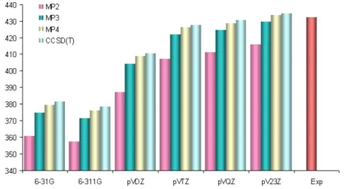
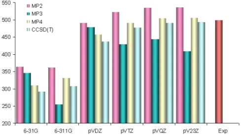
The labels pVDZ, pVTZ, pVQZ and pV23Z denote the basis sets aug-cc-pVDZ, aug-cc-pVTZ, aug-cc-pVQZ and extrapolated energies aug-cc-pV23Z, respectively. . . 89 6.2 Dissociation energies in kJ/mol of the molecules calculated at 298.15

K and 1.013 bar. Experimental dissociation energy is 432.1 kJ/mol for H 2 ; O 2 : 498.4 kJ/mol and for F 2 : 154.5 kJ/mol [47]. . . 90 6.3 Bond lengths/˚ A of the dimers H 2 -O 2 and H 2 -F 2 in an optimized T

configuration, calculated with different methods and basis sets. Ex-

perimental bond lengths are 0.7413 ˚ A, 1.2074 ˚ A and 1.418 ˚ A for

hydrogen, oxygen and fluorine, respectively [119]. . . 90

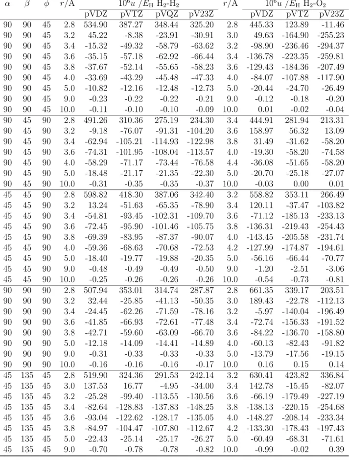
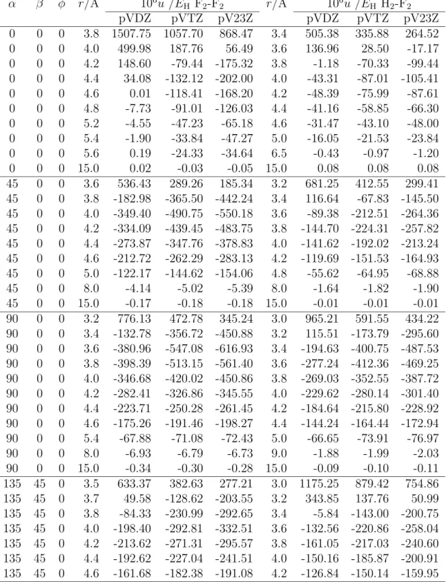
6.4 Potential energies, 10 ⁶ E min /E H and equilibrium distances, r min /˚ A of the dimers at selected orientations (α, β, φ), calculated with CCSD(T) method and basis sets aug-cc-pVm Z (m = 2, 3, 4, 23). The labels pVDZ, pVTZ, pVQZ and pV23Z denote the basis sets aug-cc-pVDZ, aug-cc-pVTZ, aug-cc-pVQZ and extrapolated energies aug-cc-pV23Z, respectively. . . 91 6.5 Pair interaction energies of dimers H 2 -H 2 and H 2 -O 2 calculated with

the CCSD(T) method and the basis sets aug-cc-pVm Z (m = 2, 3, 23) (23 denotes the extrapolation from sets 2 and 3). . . 100 6.6 Table 6.5 continued . . . 101 6.7 Table 6.6 continued . . . 102 6.8 Pair interaction energies of dimers F 2 -F 2 and H 2 -F 2 calculated with

the CCSD(T) method and the basis sets aug-cc-pVm Z (m = 2, 3, 23) (23 denotes the extrapolation from sets 2 and 3). . . 103 6.9 Table 6.8 continued . . . 104 6.10 Table 6.9 continued . . . 105 6.11 Table 6.10 continued . . . 106 7.1 Optimized parameters of the 5-site potential function Eq. 3.3 for the

dimers H 2 -H 2 and H 2 -O 2 . For all interactions δ ij = 2.0 ˚ A ⁻¹ and β = 1.0 ˚ A ⁻¹ were assumed. Partial charges: hydrogen: q N /e = -0.07833, q H = 0; oxygen: q N /e = -0.98630; q M = -2q N . E H = 4.359782 × 10 ⁻¹⁸ J (Hartree energy unit). . . 109 7.2 Optimized parameters of the 5-site potential function Eq. 3.4 for the

dimers H 2 -H 2 and H 2 -O 2 . For all interactions δ ij = 5.0 ˚ A ⁻¹ and β = 1.0 ˚ A ⁻¹ were assumed. See Table 7.1 for the partial charges. . . 110 7.3 Optimized parameters of the 5-site potential function Eq. 3.5 for the

dimers F ₂ -F ₂ and H ₂ -F ₂ . For all interactions δ _ij = 2.0 ˚ A ⁻¹ was as- sumed. Partial charges: hydrogen: q N /e = -0.078329, q H = 0; fluorine:

q N /e = -0.781897132, q F = 0; q M = -2q N . E H = 4.359782 × 10 ⁻¹⁸ J (Hartree energy unit). . . 113 7.4 Optimized parameters of the 5-site potential function Eq. 3.6 for the

dimers F 2 -F 2 and H 2 -F 2 . For all interactions δ ij = 5.0 ˚ A ⁻¹ was as-

sumed. See Table 7.3 for the partial charges. . . 114

8.1 Second virial coefficients, B ⁰ _cl of hydrogen (given in cm ³ /mol) calcu- lated from pair potentials at the level CCSD(T)/aug-cc-pVmZ (m = 2, 3, 4, 23). . . 115 8.2 Second virial coefficients of hydrogen as a function of temperature

(given in cm ³ /mol). B ⁰ _cl : classical result obtained from pair poten- tials; B ¹ _r , B ¹ _a,I , B ¹ _a,µ : quantum corrections; B: total virial coefficient;

Sph.harm: ab initio prediction of Diep and Johnson [25, 26] and Et- ters et al. [32]; exp.: experimental data. . . 116 8.3 Cross second virial coefficient (given in cm ³ /mol) of the mixture hy-

drogen–oxygen; correl.: empirical correlation [30]; exp.: experimental data. For an explanation of the other properties see Table 8.2. . . 117 8.4 Second virial coefficients, B ⁰ _cl of fluorine (given in cm ³ /mol) calculated

from pair potentials at the level CCSD(T)/aug-cc-pVm Z (m = 2, 3, 23). . . 118 8.5 Second virial coefficients of fluorine (given in cm ³ /mol). D1 EOS.:

Deiters equation of state [18]. For an explanation of the other prop- erties see Table 8.2. . . 119 8.6 Cross second virial coefficient (given in cm ³ /mol) of the mixture

hydrogen-fluorine; correl.: empirical correlation [30]. For an explana- tion of the other properties see Table 8.2. . . 120 9.1 Density results (given in g/cm ³ ) for the pure liquid estimated at two

pressures 1.0 MPa and 5.0 MPa for hydrogen, and 1.0 MPa and 10.0 MPa for fluorine using ab initio potentials, respectively; EOS : modi- fied Benedict-Webb-Rubin equation of state [139]; exp.: experimental data [17, 76]; D1 EOS: Deiters equation of state [18]. . . 134 9.2 GEMC simulation results and statistical uncertainties for hydrogen

calculated with the CCSD(T)/aug-cc-pV23Z extrapolated potentials Eq. 3.3; exp.: experimental data [76]; EOS : equation of state [139];

the values of parentheses are the uncertainty of the last digits obtained from the simulations, e.g., 0.0746(31) = 0.0746 ± 0.031. . . 135 9.3 GEMC simulation results and statistical uncertainties for hydrogen

calculated with the CCSD(T)/aug-cc-pV23Z extrapolated potentials

Eq. 3.4. For an explanation of the other properties see Table 9.2. . . . 136

10.1 GEMC simulation results and statistical uncertainties for fluorine calculated with the CCSD(T)/aug-cc-pV23Z extrapolated potentials:

Eq. 3.5; D1-EOS: Deiters equation of state [18]; exp.: experimental data [17]; the values of parentheses are the uncertainty of the last digits obtained from the simulations, e.g., 1.6152(63) = 1.6152±0.063. 150 10.2 GEMC simulation results and statistical uncertainties for fluorine

calculated with the CCSD(T)/aug-cc-pV23Z extrapolated potentials

Eq. 3.6. For an explanation of the other properties see Table 10.1 . . 151

Introduction

Hydrogen, fluorine and the mixtures hydrogen-oxygen and hydrogen-fluorine are used in several industrial areas. Hydrogen in its liquid form has been used as a fuel in space vehicles for years [95]. It could become the most important energy carrier of tomorrow [59]. Liquid hydrogen, oxygen and fluorine are the usual liquid fuels for rocket engines [122, 58, 2, 3]. The National Aeronautics and Space Adminis- tration (NASA) is the largest user of liquid hydrogen in the world [16, 41]. The knowledge of thermodynamic properties of the pure substances hydrogen, fluorine and the mixtures hydrogen-oxygen and hydrogen-fluorine are important for practi- cal applications. It is also necessary for their safe use [46, 76].

Computer simulations have expanded in number, complexity, and importance over the last many years [4]. Computers permit the study of systems for which ana- lytical solutions are not available or require approximation techniques. Molecular simulations have been used for various studies [35]. The properties of the stud- ied systems are determined solely by the intermolecular forces and energies [35, 4].

Therefore, simulations have become a necessary tool for studying fluids and fluid mixtures. They can generate structural and thermodynamic as well as transport properties consistently without the need to introduce artificial simplifications as re- quired by integral equation techniques, and statistical thermodynamic perturbation theory [35, 4]. Computer simulation techniques, Monte Carlo as well as Molecular Dynamics, cannot work without some input. It is necessary to know the interaction potentials of the systems under study.

1

Monte Carlo simulation is used to calculate widely phase equilibria of both poly- meric and low molecular organic substances. The field of phase equilibria simulation is now highly developed and very broad in techniques and applications. Some re- cently published works, are de Pablo et al. (1998 and 2000) [87, 86], Delhommelle et al. (2000) [123], Martin and Siepmann (1998 and 1999) [71, 72] and Spyriouni et al.

(1998) [112]. Gibbs ensemble simulation had been developed by Panagiotopoulos (1987) [91]. The basic idea in the Gibbs ensemble method is to simulate phase co- existence properties by following the evolution in phase space of a system composed of two distinct regions. The two regions in the simulation system represent the two coexistence phases, e.g. a vapor in equilibrium with a liquid at saturation. However, there are no physical interfaces between the two regions. In general, the two regions have different densities and compositions, while they are at thermodynamic equilib- rium with each other. Although the Gibbs ensemble simulation considers chemical equilibria between coexisting phases, it does not require an explicit calculation of the chemical potential. Due to its simplicity, the Gibbs ensemble method became the choice for simulating phase equilibria in the past decade.

Gibbs Ensemble Monte Carlo simulation has become a useful tool to estimate the phase equilibria of several pure substances and their binary and ternary mixtures.

Gibbs ensemble Monte Carlo simulation technique was used for

• Pure components: It permits simulation of vapor-liquid coexistence points for any pure component system at a given temperature.

• Mixtures: It permits simulation of vapor-liquid and liquid-liquid coexistence points for binary and ternary systems at any given temperature and pressure.

• Critical constants: It permits prediction of critical points based on a supplied set of pure component coexistence points.

Vapor-liquid equilibria can also be estimated with several equations of state and

with Monte Carlo simulation using analytic potential functions, in which the usual

procedure is to assume a simple model potential, e.g., the Lennard-Jones pair po-

tential (1924) [63] and the Morse potential (1929) [81], fit its parameters to suitable

experimental data, and then to perform the simulation. Such a simulation is no

longer predictive, because it requires an experimental input of the same kind that it

produces. This can sometimes be a severe limitation, namely if experimental data are scarce.

Recently an alternative approach has become feasible, for which the name “global simulation” has been coined by H. Popkie et al. (1973) [97]. It consists of a cal- culation of intermolecular potentials by quantum mechanical methods, followed by computer simulations and eventually calculations with equations of state fitted to the simulation results, in order to obtain properties that are not accessible to sim- ulations. Such global simulations have been reported for the noble gases, where it is now possible to predict the vapor-liquid phase equilibria without recourse to ex- perimental data with an accuracy comparable to the experimental uncertainty. One of the first attempts that achieved near-experimental accuracy was that of Deiters, Hloucha and Leonhard (1999) [23] for neon. Further global simulation attempts for noble gases were published by the groups of Eggenberger and Huber [29, 126, 96], Sandler [37], and Malijevsk´ y [69]. Using a functional form for the dispersion poten- tials of argon and krypton proposed by Korona et al. [56], Nasrabad and Deiters (2003, 2004) even predicted phase high-pressure vapour–liquid phase equilibria of noble-gas mixtures [84, 85]. Other mixed-dimer pair potentials for noble gases were published by L´opez Cacheiro et al. (2004) [7], but they were not used for phase equilibria predictions, yet.

The development of ab initio pair potentials for molecules is much more complicated because of the angular degrees of freedom of molecular motion, but for some sim- ple molecules such potentials have already been constructed: Leonhard and Deiters (2002) used a 5-site Morse potential to represent the pair potential of nitrogen [65]

and were able to predict vapour pressures and orthobaric densities. Bock et al.

(2000) also used a 5-site pair potential for carbon dioxide [5]. There have been other attempts to develop a pair potential function for hydrogen. Recently such a potential was published by Diep and Johnson (2000) [25, 26], who performed cal- culations with post-SCF methods MP2, MP3, MP4, and CCSD(T) and with the basis sets aug-cc-pVmZ (m =2, 3, 4), including extrapolation to the basis set limit.

This pair potential, however, uses a spherical harmonics expansion to account for

the anisotropy of interaction. Such an approach can become problematic, however,

if repulsion at short ranges becomes the dominant feature of a fluid, e.g., in a dense

liquid state; they furthermore applied the first-order quantum correction to the 2nd virial coefficients developed by Pack (1983) [89] and Wang Chang [45]. Naicker et al. (2003) [83] used SAPT (symmetry-adapted perturbation theory) to develop a 3- site pair potential for hydrogen chloride, based on Korona’s function and a modified Morse potential; they then successfully predicted the vapour–liquid phase equilibria of hydrogen chloride with GEMC (Gibbs ensemble Monte Carlo [92]) simulations.

Research objectives

The ab initio intermolecular pair potentials of the dimers H 2 -H 2 , F 2 -F 2 , H 2 -O 2

and H 2 -F 2 should be calculated from quantum mechanics, using the level of theory CCSD(T) and correlation-consistent basis sets aug-cc-pVmZ (m = 2, 3, 4). Then the quantum mechanical results should be used to construct four new analytical potential functions of these dimers. The second virial coefficients of the dimers H 2 - H 2 , F 2 -F 2 and the cross second virial coefficients of the dimers H 2 -O 2 and H 2 -F 2

have to be determined by integration of these functions. The thermodynamics of vapor-liquid equilibria as well as the structural properties of pure fluids hydrogen and fluorine should be derived from GEMC simulations using those potentials.

To achieve these goals, the thesis has the following four specific objectives:

• Calculations from quantum mechanics: Constructing the angular orientations of the dimers H 2 -H 2 , H 2 -O 2 , F 2 -F 2 and H 2 -F 2 ; calculating the ab initio inter- molecular energies for all built orientations, and single-molecule properties of some representational orientations from quantum chemical methods CCSD(T), MPn (n =2, 3, 4) and basis sets; correcting the energy results for the basis set superposition error (BSSE) with the counterpoise method; extrapolating the interaction energies to the complete basis set limit aug-cc-pV23Z.

• Construction of analytical potential functions: Developing four new 5-site ab initio intermolecular potentials of the dimers H 2 -H 2 , H 2 -O 2 , F 2 -F 2 and H 2 -F 2

along the proposed potentials of carbon dioxide [5], nitrogen [65] and hydrogen

chloride [83]; estimating the adjustable parameters of these analytical poten-

tial functions with the fit to ab initio intermolecular energies combining the

Levenberg-Marquardt (LM) and the Genetic Algorithm (GA); evaluating the

accuracy of the fit upon the statistical results of analysis.

• Prediction of virial coefficients: Calculating the second virial coefficients of hydrogen, fluorine and the cross second virial coefficients of the dimers hy- drogen–oxygen and hydrogen-fluorine by 4D numerical integrals for the con- structed potential functions; eventually including corrections for quantum ef- fects; comparing the accuracy of the obtained virial coefficients of this work with the experimental data and with results from the correlation equations and equations of state.

• Simulation of the phase equilibria: Carrying out GEMC-NPT and NVT sim- ulations using the four developed ab initio 5-site intermolecular potentials of hydrogen and fluorine for the temperature range from 18 K to 32 K for hy- drogen and from 60 K to 140 K for fluorine; calculating the thermodynamic properties and the critical point of the fluids hydrogen and fluorine from the obtained densities of coexisting phases and vapor pressures; comparing the results in this work with experimental data and with results from equations of state.

Outline of the thesis

This thesis consists of five chapters and five appendices.

Chapter 1: This chapter gives an introduction to important applications and proper- ties of hydrogen, oxygen and fluorine, and their mixtures; it presents the simulation methods are being used recently for the prediction of the thermodynamic properties of several systems; also the major objectives of this thesis are shown in here.

Chapter 2: This chapter describes the theoretical background for the ab initio calcu- lations, the basis sets and the intermolecular pair potentials, for the calculations of the second virial coefficients with quantum effects, the equations of state, Levenberg- Marquardt (LM) and the Genetic Algorithm (GA) used for the least-square fit, the Metropolis algorithm, and the Gibbs ensemble Monte Carlo simulations.

Chapter 3: This chapter contains the methodologies, requirements and means of

calculation, in which all are extracted upon the theoretical background; the com- puter programs and materials used for this thesis are shown here; the four new in- termolecular potentials used for the calculation of the virial coefficients and GEMC simulations are shown here too; this chapter also contains the simulation details which are needed for the prediction of the vapor liquid equilibria.

Chapter 4: This chapter presents the discussion following the calculation results which have been obtained from the performing stages. The results are compared with experimental data.

Chapter 5: This chapter summarizes and discusses the achievements of the the-

sis, and gives recommendation for future work.

Theoretical Background

2.1 Ab initio implementations

Quantum mechanics (QM) provides an accurate mathematical description of the behavior of electrons. QM is used in chemistry to predict many properties of an individual atom or molecule. In practice, the QM equations can only be solved ex- actly for one-electron systems. QM methods have been developed for approximating the solutions for multiple-electron systems. The energies and wave-functions of a system are given by the solutions of the Schr¨odinger Equation [43, 14]:

HΨ = b EΨ (2.1)

where H b is the Hamiltonian operator, which in this case gives the kinetic and po- tential energies of atomic nuclei and electrons. The wave-function Ψ depends on the coordinates of the electrons and the nuclei. The Hamiltonian consists of kinetic and potential energy terms, in general,

H b = − h ² 8π ²

particles X

i

1 m i

µ ∂ ²

∂x ² _i + ∂ ²

∂y _i ² + ∂ ²

∂z ² _i

¶

+ 1

4πε 0

particles X X

i<j

q i q j

r ij

(2.2)

where m i and q i are the mass and charge of particle i, and r ij is the distance of be- tween particles. The first term gives the kinetic energy of the particle. The second term represents the Coulombic attraction or repulsion of particles.

The Born-Oppenheimer approximation simplifies Eq. 2.3 by separating the nuclear

7

and electron motions. The Hamiltonian for a molecule with stationary nuclei is H b = − 1

2

electrons X

i

µ ∂ ²

∂x ² _i + ∂ ²

∂y _i ² + ∂ ²

∂z _i ²

¶ 2

−

nuclei X

i

electrons X

j<i

Z i

r ij

+

electrons X X

i<j

1 r ij

(2.3)

Here the first term corresponds to the kinetic energy of the electrons, the second to the attraction of electrons to nuclei, and the third to the repulsion between electrons.

The repulsion between nuclei is defined at the end of the calculation [43, 14, 13, 48].

2.1.1 Electron correlation methods

The Hartree-Fock method provides approximate solutions to the Schr¨odinger equa- tion by replacing the real electron-electron interaction with an average interaction.

The Electron Correlation (EC) energy is the energy difference between the HF and the lowest possible energy in each basis set. It is due to a correlation between the motion of electrons. For systems and states where correlation effects are important, the Hartree-Fock results will not be satisfactory [34]. QM methods have been de- veloped to include some effects of electron correlation [13, 48, 34].

Three main correlation correction methods are Configuration Interaction (CI), Many Body Perturbation Theory (MBPT), and Coupled-Cluster (CC). The Coupled- Cluster method presents the most successful approach to accurate many-electron molecular solutions. It might applied to relatively large systems and is capable of recovering a large part of the correlation energy [13, 48, 34].

In practice the Coupled-Cluster method is restricted to large systems with multi- electron configurations. However the Coupled-Cluster wave function provides an accurate correlation to the Hartree-Fock description [13, 48, 34].

Configuration Interaction (CI)

Configuration Interaction (CI) methods constructed by replacing one or more occu-

pied orbitals in Hartree-Fock determinant with a virtual orbital. The wave function

of the system is represented as the linear combination of these multiple determi- nants [13].

Ψ = c 0 Ψ HF + c 1 Ψ 1 + c 2 Ψ 2 + ... (2.4)

Here the coefficients c i are the weights of each determinant in the expansion and ensure normalization.

The full CI method builds wave-functions by the linear combination of the Hartree- Fock determinant and all possible substituted determinants [48, 13];

Ψ = c 0 Ψ HF + X

s>0

c s Ψ s (2.5)

Here the first term in right side is the Hartree-Fock determinant, and s runs over all possible substitutions.

Møller–Plesset perturbation theory

Møller and Plesset (1934) [48, 13] proposed a convection for correlation as a pertur- bation from the Hartree-Fock wave-function. It is called Møller–Plesset perturbation theory. The minimal correlation is the second-order MP2 method. Third-order MP3 and fourth-order MP4 calculations are also possible. The results of an MP4 calcu- lation is equivalent to a CISD calculation. MP5 and higher calculations are seldom carried out due to the high computation time [62, 48].

In the Møller–Plesset perturbation theory the perturbed Hamiltonian, H λ is defined as

H λ = H 0 + X ∞

i=1

λ ⁱ H i (2.6)

Here λ is an expansion coefficient. The n-electron integral over H 0 is equal to the sum over the one-electron eigenvalues of the Fock Operator.

The exact ground-state wave function and energy Ψ _λ and E _λ of a system described

by the full Hamiltonian H λ can be expanded in powers of λ [62, 34].

Ψ λ = Ψ ⁽⁰⁾ + λΨ ⁽¹⁾ + λ ² Ψ ⁽²⁾ + ...

E λ = E ⁽⁰⁾ + λE ⁽¹⁾ + λ ² E ⁽²⁾ + ... (2.7)

Insertion of the exact wave function and energy into the Schr¨odinger equation yields (H ₀ + λV )(Ψ ⁽⁰⁾ + λΨ ⁽¹⁾ + ...) = (E ⁽⁰⁾ + λE ⁽¹⁾ + ...)(Ψ ⁽⁰⁾ + λΨ ⁽¹⁾ + ...) (2.8) After expanding the results, the coefficients on each side of the equation can be equated for each power of λ, leading to a set of relations representing successively higher orders of perturbation.

(H 0 + λE ⁽⁰⁾ )Ψ ⁽⁰⁾ = 0

(H 0 + E ⁽⁰⁾ )Ψ ⁽¹⁾ = (E ⁽¹⁾ − V )Ψ ⁽⁰⁾

(H 0 + E ⁽⁰⁾ )Ψ ⁽²⁾ = (E ⁽¹⁾ − V )Ψ ⁽¹⁾ + E ⁽²⁾ Ψ ⁰

(2.9)

The correction of energy and wave function at corresponding order can be obtained by solving the equation for each order of λ, [13, 34].

Coupled-Cluster theory

Today, Coupled-Cluster (CC) theory is probably the most accurate and best appli- cable approach for the treatment of molecular systems. The Coupled Cluster (CC) method was developed in the late 1960s by Cizek (1966) [11, 13, 48], but it was not until the late 1970s that the practical implementation began to take place and until 1982 that the key stone of modern implementation, CCSD (Coupled Cluster with single and double excitation) [98], was presented.

The size consistency problem of CI is solved by using the CC method to form a wave-function where the excitation operators are exponentiated [11, 13, 48]

ψ _CC = exp(T )ψ _C (2.10)

The cluster operator T is defined as T = T 1 + T 2 + T 3 + ... + T n

and T _n is a linear combination of all n-type excitations. n the total number of

electrons and the various T i operators generate all possible determinants having i excitations from the reference.

T 1 Ψ C = X

i

X

a

C ^a _i Ψ i

T 2 Ψ C = X

i>j

X

a>b

C ^ab _ij Ψ ^ab _ij (2.11)

Here C ^a _i and C ^ab _ij are the coefficients to be determined Ψ CCSD = Ψ 0 + X

a

X

i

C ^a _i Ψ ^c _i + X

i>j

X

a>b

C ^ab _ij Ψ ^ab _ij + 1

2 X

cb

X

ij

C ^c _i C ^b _j Ψ ^cb _ij + 1 2

X

a>b

X

c>d

X

i>j

X

k>l

C ^ij _ab C ^kl _cd Ψ ^abcd _ijkl + . . .

(2.12)

This appears to be the advantage of CC theory: Higher excitations are included, but their coefficients may be determined by the excitations of lower order. The coefficients are determined by projecting Schr¨odinger’s equation on the left with the configurations generated by the ˆ T operator. This replaces the eigenvalue problem by a non-linear simultaneous system [39].

Coupled cluster calculations can be similar to configuration interaction calculations, in which the wave function is a linear combination of many determinants [13, 34, 48].

The method used in this work, CCSD(T), includes triple excitations perturbatively rather than exactly. Coupled Cluster calculations give variational energies as long as the excitations are included successively [13, 34, 48].

2.1.2 Basis sets

Ab initio methods try to get accurate information by solving the Schr¨odinger equa-

tion without fitting parameters to experimental data. Actually, ab initio methods

also make use of experimental data in a rather subtle way. These methods use

several approximations for solving the Schr¨odinger equation. One of the approxi-

mations inherent in essentially all ab initio methods is the use of basis sets [13, 48].

An individual molecular orbital is defined as [34]:

ψ i = X N µ=1

c µi Φ µ (2.13)

here the coefficients c µi are known as the molecular orbital expansion coefficients.

The basis functions Φ 1 ... N are assumed to be normalized. Thus Φ µ refers to an arbitrary basis function in the same way that ψ i refers to an molecular orbital.

In HF calculations the wave function need to be described by mathematical func- tions, which are known well for a few one-electron systems only. This is the second approximation of the HF calculation. The functions used most often are linear com- binations of Gaussian-type orbitals exp(−ar ² ), denoted GTO. Amongst the used split-valence basis sets are those of Pople et al. [13] including the basis sets 3-21G, 6-21G, 4-31G, 6-31G, and 6-311G. The first number indicates the number of primi- tives used in the contracted core functions. The numbers after the hyphen indicate the numbers of primitives used in the valence functions. If there are two numbers, it is a valence-double-ζ basis, is there are three, valence-triple-ζ [13, 34, 48].

Split-valence basis set: the 6-31G basis sets

For the basis set 6-31G the core orbitals are a contraction of six primitive GTOs (PGTOs), the inner part of the valence orbitals is a contraction of three PGTOs and outer part of the valence is represented by one PGTO. The designation of the car- bon/hydrogen 6-31G basis is (10s4p/4s) → [3s2p/2s]. This basis set is only strictly defined for hydrogen through fluorine [48, 13].

The basis set 6-31G(p1,p2) where p1 can be d, 2d, 3d, f, df, 2df or 3df and p2

can be p, 2p, 3p, d, pd, 2pd or 3pd. 6-31G* can be used instead of 6-31G(d) and

6-31G** is the same as 6-31G(d,p). The 6-31+G basis will add diffuse s- and p-

orbitals on all non-hydrogen atoms and 6-31++G also adds diffuse s-functions on

all hydrogen atoms [48].

Split-valence basis set: the 6-311G basis sets

For the basis set 6-311G the core orbitals are also a contraction of six primitive GTOs (PGTOs); This basis set is only strictly defined for hydrogen through fluo- rine [48, 13].

The general form of the basis set is 6-311G(p1,p2) where p1 can be d, 2d, 3d, f, df, 2df or 3df and p2 can be p, 2p, 3p, d, pd, 2pd or 3pd. 6-311G* can be used instead of 6-311G(d) and 6-311G** is the same as 6-311G(d,p). The 6-311+G basis will add diffuse s- and p- orbitals on all non-hydrogen atoms and 6-311++G also adds diffuse s-functions on all hydrogen atoms [48, 13].

Correlation consistent basis sets

A set of basis sets for correlated calculations has also been developed by Dunning et al (1970) [51, 52, 53]. These basis sets are called as correlation consistent (or cc) and are designed as a base set of sp functions combined with correlation functions.

Several basis sets of different sizes are available. These are known by their ab- breviation: cc-pVDZ, cc-pVTZ, cc-pVQZ, and cc-pV5Z, where D, T and Q indicate the number of contracted functions. The terms of primitive and contracted functions are shown below [48, 13].

Basis Primitive functions Contracted functions

cc-pVDZ 9s,4p,1d/4s,1p 3s,2p,1d/2s,1p

cc-pVTZ 10s,5p,2d,1f/5s,2p,1d 4s,3p,2d,1f/3s,2p,1d cc-pVQZ 12s,6p,3d,2f,1g/6s,3p,2d,1f 5s,4p,3d,2f,1g/4s,3p,2d,1f cc-pV5Z 14s,9p,4d,3f,2g,1h/8s,4p,3d,2f,1g 6s,5p,4d,3f,2g,1h/5s,4p,3d,2f,1g The energy–optimized cc basis sets are augmented by additional diffuse functions, denoted by the prefix aug- to the abbreviation. The augmentation involves inserting one extra function with a smaller exponent for each angular momentum [48].

2.1.3 Supermolecule approach

In calculations for dimers, basis functions of one molecule can be contribute to the

basis set of the other. The effect is known as Basis Set Superposition Error (BSSE).

In the limit of a complete basis set, the BSSE would be zero [48, 13, 43]. An approximate method of assessing BSSE is the counterpoise (CP) correction. The BSSE is estimated from the monomer energies with the regular basis and the energies calculated with the full set of basis functions for the whole complex. The geometries of the two separated molecules A and B, and the complex AB are optimized. The energy difference between those is calculated with following formula [48, 13, 60, 43]

∆E = E(AB) ^∗ _ab − E(A) a − E(B) b (2.14)

Here basis set a for A and basis set b for B, and basis set ab for complex AB. Two energy calculations of the fragments in the complex are carried out with the full ab basis set. The energy of A is calculated in the presence of both the normal a basis functions and with the b basis functions of fragment B located at the corresponding nuclear positions, but without the B nucleus present. Such basis functions located at fixed points in space are referred to as ghost orbitals. The CP correction is calculated as [48, 13, 43]

∆E CP = E(A) ^∗ _ab + E(B) ^∗ _ab − E (A) ^∗ _a − E(B) ^∗ _b (2.15) The counterpoise corrected ∆E energy is given as ∆E − ∆E CP [48, 13, 43].

2.1.4 Symmetry-adapted perturbation theory

This perturbational method was proposed by Jeziorski et al. [49, 50, 120]. It com- putes the interaction energy E int directly from a sum of physical contributions

E int = E _pol ⁽¹⁾ + E _exch ⁽¹⁾ + E _pol ⁽²⁾ + E _exch ⁽²⁾ + · · · (2.16) where E _pol ⁽¹⁾ is the damped classical electrostatic interaction energy, E _pol ⁽²⁾ is a sum of the damped classical induction and quantum mechanical dispersion energies

E _pol ⁽²⁾ = E _ind ⁽²⁾ + E _disp ⁽²⁾ (2.17)

and E _exch ⁽ⁿ⁾ , n = 1,2, are exchange corrections defined by the symmetry-adapted

perturbation theory (SAPT) [49, 50, 120].

2.1.5 Extrapolation to the basis set limit

Many attempts were to extrapolate the interaction energies of weakly bound molec- ular system at the basis set limit from correlation-consistent basis sets and an ex- trapolation scheme. The relationship between the correlation-consistent energies and the energy in the basis-set limit may now be written as [43, 138, 55, 10]

∆E exact = ∆E X + AX ⁻³ (2.18)

Using this formula, the correlation energy E exact can be extrapolated from the correlation-consistent energies E X for small cardinal numbers X. To apply Eq. 2.18, only two energies are needed. From the cardinal numbers X and Y, the energies E X and E Y can be obtained. From these energies, the extrapolated basis-set limit E _XY ^∗ and the parameter A XY can be determined with the following two equations satisfied [43, 138, 55, 10, 33]

E _XY ^∗ = E X + A XY X ⁻³ (2.19)

E _XY ^∗ = E Y + A XY Y ⁻³ (2.20)

The extrapolated correlation energy and the linear parameter A XY can be calculated from the following formulae [43, 10]:

E _XY ^∗ = X ³ E X − Y ³ E Y

X ³ − Y ³ and A _XY = E X − E Y

X ⁻³ − Y ⁻³ (2.21)

2.1.6 Electrostatic interactions

Electrostatics is the study of interactions between charged positions. It is necessary for understanding the interactions of electrons, which is described by a wave func- tion or electron density. The Coulomb’s law equation for the energy of interaction between two particles with charges e a and e b at a distance r ab is [114]

E = 1 4π² 0

X

a∈A

X

b∈B

e a e b

r ab (2.22)

2.2 Intermolecular potential functions

2.2.1 Lennard-Jones potential

The total intermolecular pair potential is obtained by summing the attractive and repulsive potentials. One of them is the Lennard-Jones (1924) 6-12 potential [63].

This potential function was used successfully for noble gases, but also in simulations of molecules, by using 2-site models [9, 79] by adding quadrupole moments [8, 57].

The Lennard-Jones potential can be written as E _ij = 4²

"µ σ r ij

¶ 12

− µ σ

r ij

¶ 6 #

(2.23) where ² characterises the well depth of the pair interaction and σ is the hard sphere radius of the atom (the distance at which E ij is zero). r ij is the distance between i and j (r ij = |~r i − ~r j |).

In 1987 the Gibbs ensemble Monte Carlo technique was proposed by Panagiotopou- los [91]. The phase properties of several systems have been obtained successfully by these techniques using Lennard-Jones 6-12 potentials.

2.2.2 Morse potential

The harmonic potential is a starting point for a discussion of vibrating molecules.

A potential that is suitable for cases when attractive interaction comes from the formation of a chemical bond was proposed by Morse (1930) [81]:

E ij = D

· e ^−2α

³

re

´

− 2e ^−α

³

re

´ ¸

, (2.24)

The Morse potential is usually written as [44]

E _ij = D(1 − exp(−αr _ij )) ² (2.25)

where D is the depth of the interaction potential, r ij is the interaction distance

and α denotes the range of the interaction. This potential is widely used to model

covalently diatomic molecules. Both potentials Eq. 2.23 and 2.24 are scalable. The