Configuration Path Integral Monte Carlo

Configuration Path Integral Monte Carlo

T. Schoof¹, M. Bonitz^∗1, A. Filinov^1,2, D. Hochstuhl¹,andJ.W. Dufty³

1Institute for Theoretical Physics and Astrophysics, Christian Albrechts University Kiel, Leibnizstrasse 15, D-24098 Kiel, Germany

2Institute of Spectroscopy of the Russian Academy of Sciences, Troitsk, Russia

3Physics Department, University of Florida, Gainesville

Received 24 February 2011, revised 28 March 2011, accepted 31 March 2011 Published online 11 April 2011

Key words Dense plasmas, quantum plasmas, thermodynamic properties, path integral Monte Carlo

A novel path integral Monte Carlo (PIMC) approach for correlated many-particle systems with arbitrary pair interaction in continuous space at low temperatures is presented. It is based on a representation of theN-particle density operator in a basis of (anti-)symmetrizedN-particle states (configurationsof occupation numbers).

The path integral is transformed into a sum over trajectories with the same topology and, finally, the limit of M → ∞, whereM is the number of high-temperature factors, is analytically performed. This yields exact expressions for the thermodynamic quantities and allows to perform efficient simulations for fermions at low temperature and weak to moderate coupling. Our method is expected to be applicable to dense quantum plasmas in the regime of strong degeneracy where conventional PIMC fails due to the fermion sign problem.

c 2011 WILEY-VCH Verlag GmbH & Co. KGaA, Weinheim

1 Introduction

Nonideal many-particle systems are of rapidly increasing importance in many fields of physics and chemistry.

Examples are dense astrophysical and laboratory plasmas, many-electron atoms and molecules, nonideal Bose condensates or the quark gluon plasma, e.g. [1, 2]. Of particular importance are partially ionized plasmas pro- duced by strong electromagnetic fields e.g. [3] where nonideality (correlation) effects, electron degeneracy and exchange as well as bound state formation have to be taken into account selfconsistently. Here analytical methods or semiclasscial approaches fail, and one has to resort to first-principle approaches, see e.g. [1] for an overview.

Among them, a central role is being played by quantum Monte Carlo methods which have seen a remarkable development in recent years, e.g. [4–7], in particular in the theory of dense plasmas, e.g. [7–11].

While for bosons path integral Monte Carlo simulations (PIMC) are able to achieve virtually exact results e.g. [4, 12] fermionic simulations are hampered by the notorius fermion sign problem which prevents simulations at low temperature (strong degeneracy, see below). It is, therefore, of crucial importance, not only for plasmas but for electrons in condensed matter or multi-electron atoms as well, to develop novel concepts which may relieve the sign problem. Here we present a new approach to PIMC simulations – configuration PIMC (CPIMC) that allows to make progress in this direction. CPIMC has the following features: 1.) it uses a representation of the density operator in terms of (anti-)symmetrized N-particle states in occupation number representation, 2.) the states are constructed from an arbitrary single-particle basis. 3.) the matrix elements for an aribtrary pair interaction are efficiently computed using the Slater-Condon rules, 4.) The limitM → ∞is performed analytically (M is the number of high-temperature factors) thus leading to exact results [13].

∗ Corresponding author: E-mail:bonitz@physik.uni-kiel.de, Phone: + 49 431 880-4122, Fax: + 49 431 880-4094

2 Ab inititio thermodynamics of interacting systems

We consider a general system ofN interacting identical particles with the hamiltonian

Hˆ = ˆT+ ˆV + ˆW = ˆH0+ ˆW , (1)

Hˆ₀ = ^N

α=1

ˆh_α, Wˆ = ^N

1≤α<β

ˆ

w(|r_α−r_β|). (2)

HereV denotes an external potential andwˆthe pair interaction. The system is assumed to be in thermodynamic equilibrium at a given temperatureT, volume and particle numberN, so the central quantity is theN−particle canonical density operator

ˆ ρ= 1

Ze^−βHˆ, Z= Tre^−βHˆ, β= 1

k_BT. (3)

To account for the spin statistics of bosons (fermions), one performs an (anti-)symmetrization of the density operator,ρˆ→ρˆ^S/A= ˆS^±ρˆ, by summing over allN!particle permutations. Knowledge ofρˆ^S/Agives access to expectation values of all observables of the system via

A^S/A= Tr ˆAρˆ^S/A. (4)

The main difficulty in computing the density operator is that, in general, the two parts of the Hamiltonian do not commute

[ ˆH₀,Wˆ]= 0, (5)

which can be overcome by expressingρˆin terms of the high-temperature density operator using its path integral representation.

2.1 Path integral

The path integral representation is obtained by identically expressingρˆviaM factors corresponding to anM times higher temperature, using the identity

e^−βHˆ =

e^−MβHˆ_M

, (6)

taking advantage of the fact that, in the limit M → ∞, the well-known semiclassical result for the high- temperature density matrices of kinetic and potential energy can be used [14]. This approach has been used very successfully in combination with Metropolis Monte Carlo methods during the last more than three decades in a tremendous number of applications. The standard approach uses the coordinate representation of the density operator, i.e. introducingN-particle states|R=|r₁r₂. . . r_Nwherer_i ={r_i, s_zi}, and evaluates the density matrixρ^S/A(R, R) = R|ˆρ^S/A|Rin continuous configuration space. While for bosons virtually exact results can be achieved (limited only by the available computer power), e.g. [4, 12], for fermions there is a fundamen- tal obstacle – thefermion sign problem: the sign-alternating terms in the anti-symmetrized density operatorρˆ^A prevent exact calculations at strong quantum degeneracy, in particular the ground state limitT → 0is not ac- cessible. Numerous strategies have been proposed to perform fermionic PIMC simulations including restricted PIMC [4, 8, 9, 11], multilevel blocking algorithms [5] or direct PIMC (DPIMC) with effective quantum poten- tials [7, 10]. While these methods have achieved remarkable results in recent years, they did not overcome the inherent sign problem.

Here we propose another approach to PIMC simulations: instead of computing averages with an (anti)- symmetrized density operator, as in Eq. (4), we use the original density operatorρ, but in combination withˆ (anti-)symmetricN-particle states in the trace which leaves the result unchanged,

A^S/A= Tr ˆAρˆ^S/A= Tr^S/AAˆρ.ˆ (7)

The properN-particle states are states in Fock space [16] for which we use the occupation number representation together with a complete orthonormal set of single-particle states|φ_i, with the associated occupationsn_i, where n_i = 0,1, for fermions, andn_i = 0,1,2, . . ., for bosons. The associatedN-particle state will be denoted by

|{n}=|n₀, n₁, . . .. While the theory can be developed in complete Fock space whereNis arbitrary, here it will be advantageous to restrict ourselves to the subspace of a fixed particle numberN. This introduces a restriction on the occupation numbers, _∞

i=0ni = N. The present method resembles the configuration interaction (CI) approach to the ground and excited states of many-electron atoms in quantum chemistry [19–21]. However, our method uses a mixed ensemble and arbitrary finite temperatures. This combination of PIMC withN−particle states in occupation number space (configurations) will be called configuration PIMC (CPIMC).

2.2 Configuration Path integral

We outline the CPIMC approach for the example of the canonical partition sum which we transform according to formula (6)

Z = Tr^S/Ae^−βHˆ =

{n}

{n}|e^−βHˆ|{n}=

=

{n}

{n⁽¹⁾}

· · ·

{n^M−1}

{n}|e^−MβHˆ|{n⁽¹⁾} · · · {n^(M−1)}|e^−MβHˆ|{n}, (8)

where all sums are restricted to states with fixed particle numberN. Thus the sum is over all possible “paths”

in configuration (occupation number) space: each single-particle state|φkis represented by a closed path ofM occupation numbers{nk→n⁽¹⁾_k →n⁽²⁾_k →. . . n^(M_k ⁻¹⁾→nk}situated atM+1discrete equidistant “imaginary time slices”{β₀= 0, β₁=_M^β, β₂=^2β_M . . . β_M =β}, wheren^(M_k ⁾=n_k. Next, we evaluate the matrix elements by expanding the exponentials into a Taylor series which, for sufficiently largeM, can be terminated at linear order with an error of orderO(M⁻²),

{n}|e^−MβHˆ|{n} ≈ {n}|1− β

M( ˆD+ ˆY)|{n} ≈

≈

e^−MβD{n}, {n}={n},

−_M^βY_{n},{n}, {n} ={n}. (9)

Here the hamiltonian is split into a diagonal (Dˆ) and an off-diagonal part (Yˆ),Hˆ = ˆD+ ˆY. Instead of using the finiteM approximation, alternatively, we can restore the full exponent for the diagonal part, with an error of the same order.

1 2 3 4 5 6 7 8 9 10 11 12 13 14 15 16 17 18 19 20 {n⁽⁰⁾}

{n⁽¹⁾} {n⁽²⁾},{n⁽⁴⁾} {n⁽³⁾} {n⁽⁴⁾} state{n(i)}

l0 l1 l2 l3 l4 l5

time slice i

Fig. 1 Visualization of CPIMC. AnN-particle configuration is given by an “imaginary-time path” of occupation number states{n⁽ⁱ⁾}in the interval[0, β], the example showsM+ 1 = 20time slices. The y-axis represents an arbitrary ordering of states, i.e. states with different ordinate are different and states with the same ordinate are equal. Occupation changes occur at time slicesl1= 5, l2= 6, l3= 9, l4 = 15andl5= 19, i.e. there areK= 5kinks.

In the special case of ideal single-particle states, the kinetic energy part of the hamiltonian,Hˆ₀, is diagonal, andYˆ is due to the pair interaction hamiltonianWˆ. Yet with the choice of the (anti-)symmetric states{n}the matrix elementsY_{n},{n} are known exactly, for an arbitrary pair interactionw(r)and are given by the well- known Slater-Condon rules, e.g. [22]. They consist of three parts, one of which (Wˆ^I) is diagonal, and the other two are off-diagonal, see appendix. Correspondingly, the diagonal and off-diagonal parts of the hamiltonian becomeDˆ = ˆH0+ ˆW^IandYˆ = ˆW^II+ ˆW^III.

With these results the CPIMC representation of the partition function is fully defined, and analogous expres- sions for any observable are straightforwardly derived. Numerical results can be obtained by standard Metropolis Monte Carlo to any finite orderM. But, how about the sign problem for the case of fermions? While we have removed the original source of alternating signs by avoiding the use of the anti-symmetric density operator, in general, new sources of alternating signs have emerged: obviously, the two off-diagonal interaction contributions Wˆ^II+ ˆW^IIIcontain sign-alternating terms and, in addition, each factorY contains a negative sign. So it remains to be checked in simulations how severe this problem turns out to be.

As a first test we study the results from the diagonal terms considering a spin-polarized system. If the inter- actions are completely neglected,Wˆ → 0, the thermodynamical quantities are straightforwardly evaluated. In particular, the mean occupation numbersniturn out to be given exactly by the canonical distribution of an ideal gas (in a grand-canonical simulation we recover the Fermi distribution). Note that the limitT → 0poses no difficulty at all. It has no sign problem – in striking contrast to traditional continuous space PIMC. A first improvement is achieved by including interactions within the diagonal approximations, Wˆ → Wˆ^I, then still Y ≡0. This results in a renormalization of the single-particle energies, similar to the Hartree-Fock approxima- tion. The corresponding occupation numbers are again straightforwardly computed and are, for weak coupling, indeed close to Hartree-Fock results; details will be given in Ref. [23]. Here we will concentrate on the more challenging treatment of the full interaction, including all off-diagonal terms.

3 Kink-based continuous-time CPIMC

Rather than directly evaluating expression (8) with the matrix elements (9) it turns out to be advantageous to first perform a number of reorderings and resummations.

3.1 Kink based path integral

Evidently, intervals in imaginary time within which the occupation numbers do not change involve only the diagonal partDˆ of the hamiltonian leading to ideal-like contributions which do not pose a problem. Therefore, the main challenge is to treat the occurences of changes in the occupation numbers. Letl1, . . . , lKbe the time slices that have occupation numbers different from the previous time slice, i.e.{n⁽ⁱ⁻¹⁾} ={n⁽ⁱ⁾}for alli=l1, . . . , lK

and{n⁽ⁱ⁻¹⁾}={n⁽ⁱ⁾}for alli=l₁, . . . , l_K. The positionsl₁, . . . , l_Kwill be called “kinks”. It is clear that the result for the partition function depends only on the number of kinks and on the length of the intervals in between them. We, therefore, reorder the partition function such that terms with the same number of kinks are grouped together [17]

Z= ^M

K=0K=1

(−1)^{K M}

l1=1

M l2=l1+1

. . . ^M

lK=lK−1+1

β M

_K

×

{n}=

{n(0)}={n(K)}

{n(1)}=

{n(0)}

· · ·

{n(K−1)}=

{n(K−2)},{n(K)}

e^{−Mβ Ki=0D{n(i)}(li+1−li−1)}

K−1 i=0

Y_{n⁽ⁱ⁾_},{n⁽ⁱ⁺¹⁾_}. (10)

Note that since the initial and final configuration of a path have to coincide no paths with a single kink are allowed.

This is the second equivalent result for the partition function which can be used for finiteM calculations.

3.2 TransitionM → ∞

A third expression is obtained by noting that, in Eq. (10), the limitM → ∞can be performed by replacing the discrete imaginary times of the kinks by continuous variables and the summations by integrations,

β

Mli−−−−→M→∞ τi, M li=li−1

β M

−−−−→M→∞

_β

τi−1

dτi. (11)

As a result, the expression for the canonical partition function is written as “continuous time path integral” [13,25]

which is exact Z= ^∞

K=0K=1

(−1)^K _β

0 dτ_{1 β}

τ1

dτ₂· · · _β

τK−1

dτ_K×

{n}=

{n(0)}={n(K)}

{n(1)}=

{n(0)}

· · ·

{n(K−1)}=

{n(K−2)},{n(K)}

e^{−Ki=0D{n(i)}(τi+1−τi)}·^K−1

i=0

Y_{n(i)},{n⁽ⁱ⁺¹⁾} (12)

=·.

Thus the partition function is written as a sum over continuous “trajectories” in occupation number space. Each such configuration trajectoryCI is characterized by a set of parametersIand the associated weightWI,

CI : I = {K, τ1, τ2, . . . τK,{n⁽⁰⁾}, . . .{n^(K−1)}}, W_I =W(C_I) = (−1)^Ke⁻

K

i=0D_{n(i)}(τi+1−τi)

·^K−1

i=0

Y_{n(i)},{n⁽ⁱ⁺¹⁾}. (13)

Below we will use the short notation·for the thermodynamic average in the canonical ensemble (N is fixed) over all tractoriesC_I. With the result (12), in principle, exact thermodynamic computations for interacting Fermi or Bose systems can be performed. Sources of alternating signs remain in two places: inY and in the factor (−1)^Kthe sign of which depends on the number of kinks of a path.

3.3 Expectation values of observables

Let us present a few important examples of thermodynamic quantities. The first is the expectation value of the occupation numbers

ˆnp(β, N) = 1

β K i=0

n⁽ⁱ⁾_p (τi+1−τi)

, (14)

where the thermodynamic average of Eq. (12) has been used. For each configuration the occupation number of any orbital is just the (integer) occupation number of straight pieces of the trajectory weighted by their length.

Next, consider the expectation value of the total energy which is straightforwardly computed H(β, Nˆ ) =− ∂

∂βlnZ= 1

β K

i=0

D_{n(i)}(τ_i+1−τ_i)−K β

. (15)

The result contains contributions from the (Hartree-Fock-type) diagonal terms weighted by the interval length whereas the off-diagonal contributions from the pair interaction enter only via the number of kinks of the given trajectory. Thus a central role is being played by the average number of kinksK(β, N). Similarly, we obtain for the heat capacity

Cv(β, N) = 1 T²

( ˆH− Hˆ)²− K β²

, (16)

and analogous expressions are derived for other quantities. Of central importance for the performance of the CPIMC concept is theaverage signwhich is the difference of the fractionss^±of trajectoriesC_I with a positive weight and those with a negative weight,

s(β, N) =s⁺−s⁻. (17)

This quantity – together with its variance σ_s – is a sensitive indicator for the efficiency of the Monte Carlo procedure for fermions. The fermion sign problem just corresponds to vanishing ofs. An increase ofσ_s/s causes an increase of the error of any observable.

3.4 Monte Carlo procedure

Let us outline the main ingredients for a Metropolis Monte Carlo scheme within CPIMC.

1. The first step consists in choosing a basis of single particle states{|φ}which is adopted to the system. This can be a basis of the noninteracting system, a basis of Hartree-Fock orbitals etc. The dimensionNbof the basis depends on the particle numberN and temperature. All matrix elements of kinetic and interaction energy in this basis are precomputed and stored in a table.

2. From these basis states we construct the N-particle states {n⁽ⁱ⁾} as Slater determinants in the case of fermions or permanents in the case of bosons.

3. The system is initialized in a configurationC_Iwith occupation numbers corresponding e.g. to an ideal Fermi (Bose) gas for the given temperature and basis set without kinks.

4. To generate a new trajectoryC_I, newN-particle states are generated. Depending whether these states co- incide with or differ from the left and right neighboring states the number of kinks is changed appropriately.

Depending on the weightW_Ithe new configuration is accepted or discarded.

5. Operations with kinks: to efficiently sample the whole space ofN-particle states in an ergodic manner we use three different procedures: shift of a kink, addition (removal) of one kink and addition (removal) of two kinks.

6. During the Markov process all expectation values of interest, including their statistical errors, are generated.

In particular, the average signsof the sampled trajectories, Eq. (17), is computed.

Details of the procedure, including the acceptance probabilities of the different MC moves and issues of ergodicity will be presented in Ref. [23].

4 Coulomb interacting fermions in a 1D harmonic potential

To perform a rigorous test of the CPIMC concept we considerNspin-polarized electrons in a 1D harmonic trap.

For this system with small particle numbers exact results from configuration interaction calculations and from direct PIMC simulations will be obtained below and used as a benchmark for CPIMC. Besides, this system is presently of substantial interest in ultracold atoms in optical lattices or electrons in quantum wires.

4.1 Hamiltonian and units

The hamiltonian of N identical particles with Coulomb interaction in a one-dimensional harmonic oscillator potential is given by

Hˆ =1 2

N α=1

(ˆp²_α+ ˆx²_α) +

1≤α<β

λ

|ˆx_α−xˆ_β|²+κ², (18) where we introduced standard dimensionless units and used a standard regularization of the Coulomb potential in1Dwithκ= 0.1. There are two relevant ratios of energy scales: the ratio between Coulomb interaction and oscillator energy given by the coupling parameter in the trap,λ=EC/ω, whereEC=e²/r0andr²₀=/mω, and the temperature in units of the trap energy,β=ω/kBT.

4.2 Reference data from configuration interaction and direct PIMC simulations

To have a rigorous test for the quality of the CPIMC algorithm we have performed independent first principle sim- ulations. The first are from a Configuration Interaction procedure, which has been extended to describe finite tem- peratures in the canonical ensemble [23]. Thereby, we constructed the Hamiltonian as a matrix{n}|H|{n} in the full configuration space and obtained the density operator, Eq. (3), straightforwardly by calculation of the matrix exponential. Note that the density operator obtained this way is exact up to the choice of the single-particle basis. The matrix exponential itself is evaluated through direct diagonalization of the Hamiltonian, which cor- responds to an exact solution of the Schr¨odinger equation. Obviously, this procedure is feasible only for small systems, as the effort increases exponentially with the particle numberN and with the single-particle basis size Nb(which is determined by the temperatureT) [27]. An important advantage of this comparison is that, by using the same single-particle basis as in CPIMC, we can eliminate any ambiguities due to the choice of the basis.

The second set of reference data is obtained from standard direct fermionic PIMC simulations (DPIMC) in continuous coordinate space. This method has the fermion sign problem, so simulations become increasingly inefficient with decreasing temperature andλ. In particular, the limit of the ground state of the ideal Fermi gas is not accessible. Details of our DPIMC simulations can be found in Ref. [15].

4.3 CPIMC Results

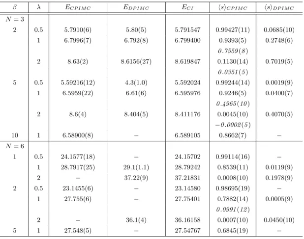
Table 1 Total energy of three and six fermions in a harmonic trap for different coupling parametersλand inverse tem- peraturesβ. Comparison of CPIMC results with direct PIMC in coordinate space (DPIMC) and configuration interaction calculations (CI). Last two columns show the average sign of CPIMC and DPIMC. For CPIMC results with Hartree-Fock orbitals are shown and, for comparison, a few from an ideal basis (lower lines, italic). MC data are for simulations with one million configurations. Missing data (dashes) indicate a relative error exceeding100%.

β λ ECP IMC EDP IMC ECI sCP IMC sDP IMC

N= 3

2 0.5 5.7910(6) 5.80(5) 5.791547 0.99427(11) 0.0685(10)

1 6.7996(7) 6.792(8) 6.799400 0.9393(5) 0.2748(6)

0.7559(8)

2 8.63(2) 8.6156(27) 8.619847 0.1130(14) 0.7019(5)

0.0351(5)

5 0.5 5.59216(12) 4.3(1.0) 5.592024 0.99244(14) 0.0019(9)

1 6.5959(22) 6.61(6) 6.595976 0.9246(5) 0.0400(7)

0.4965(10)

2 8.6(4) 8.404(5) 8.411176 0.0045(10) 0.4070(5)

−0.0002(5)

10 1 6.58900(8) − 6.589105 0.8662(7) −

N= 6

1 0.5 24.1577(18) − 24.15702 0.99114(16) −

1 28.7917(25) 29.1(1.1) 28.79242 0.8539(11) 0.0119(9)

2 − 37.22(9) 37.21831 0.0008(10) 0.1978(9)

2 0.5 23.1455(6) − 23.14580 0.98695(19) −

1 27.755(6) − 27.75401 0.7882(14) 0.0005(9)

0.0991(12)

2 − 36.1(4) 36.16158 0.0007(10) 0.0450(10)

5 1 27.548(5) − 27.54767 0.6845(19) −

We have performed a large series of simulations in a broad range of coupling parameters and temperatures.

In a first analysis we used free (ideal) one-particle states as a basis with the basis dimensionN_b = 14. The anti-symmetric N-particle states are constructed from these orbitals as Slater determinants. The total energy from CPIMC simulations is presented in table 1 and compared with exact CI results with the same single-particle basis. CPIMC shows very good agreement with CI for weak and moderate couplingλ ≤ 2, forN = 3and λ≤1, forN = 6. For larger coupling the error quickly increases (for a fixed number of Monte Carlo steps). For comparison, in table 1 we also included direct PIMC results for the same parameters. It turns out that DPIMC agrees well with CI for large coupling, but exhibits increasingly large deviations whenλis reduced. The reason of this behavior is the fermion sign problem which is analyzed in detail below, in Fig. 4.

0 0.2 0.4 0.6 0.8 1

0 2 4 6 8 10 12

A v erage o ccupation n u m b er, n

Orbital index, i

CI CPIMC β = 1 β = 2 β = 5 β= 10

N = 3

N = 6

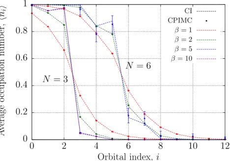
Fig. 2 Mean occupation numbers of a moderately coupled (λ= 1) systems of3and6fermions versus single particle state index and various temperatures shown in the figure. Comparison of CPIMC results using ideal states (symbols) and CI results (lines). Error bars indicate the statistical error of the simulations. (Online colour: www.cpp-journal.org).

Next, consider the mean occupation numbers which are a very sensitive test to the quality of our method.

Results for three and six particles at moderate coupling,λ= 1are shown in Fig. 2. The CPIMC results again agree very well with thermodynamic CI calculations, in particular for weak to moderate couplingλ≤ 2. The results are plotted versus the index of the single particle states (i.e. the oscillator eigenstate which are ordered by energy). As expected, for increasingβ the distribution tends towards a step-like function which, however, is broadened around the Fermi edge due to Coulomb correlations. Also, an increase of the particle number shifts the Fermi edge to higher energies. Interestingly, for an ideal basis, the occupation numbers are not monotonic which is confirmed by CI. We now repeat the simulations by using, instead of an ideal basis, Hartree-Fock states.

The results are shown in Fig. 3. and exhibit much lower statistical errors than the ideal basis calculations and agree much better with CI. In this case the mean occupation numbers are a strictly monotonic function of energy.

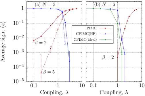
To analyze how severe the fermion sign problem is in the present CPIMC approach we compute the average sign s, Eq. (17), which is observed during the simulations, see also the data in table 1. We observe a fast decay of the average sign withT,λandN at fixed other parameters. To quantify this behavior we show the dependence ofsas a function of the coupling parameter for two constant temperaturesk_BT = 0.5ωandk_BT = 0.2ω, cf. Fig. 4. The figure shows that for weak and moderate coupling the average sign is close to unity, confirming again that simulations of an ideal or weakly nonideal strongly degenerate Fermi system pose no problem for CPIMC. At the same time we observe an exponential decrease of the sign for largerλ. In the figure we show results obtained within a Hartree-Fock single-particle basis. This gives a dramatic improvement compared to an ideal basis which is demonstrated for a few cases in table 1. In Fig. 4 we also include the average sign of DPIMC simulations.

0 0.2 0.4 0.6 0.8 1

0 2 4 6 8 10 12

A v erage o ccupation n u m b er, n

Orbital index, i

CI CPIMC β= 1 β= 2 β= 5 β= 10

N = 3

N = 6

Fig. 3 Mean occupation numbers for3and6fermions atλ= 1and various temperatures shown in the figure. Comparison of CPIMC results (symbols) and CI results (lines). HF-basis states are used. Error bars indicate the statistical error of the simulations. Note that the same orbital index forN = 3andN = 6refers to different wave functions. (Online colour:

www.cpp-journal.org).

Interestingly, these simulations show the opposite behavior: for strongly coupled states where the particles are localized and experience only little wave function overlap the average sign is large, and efficient simulations are possible. However, when the coupling parameter is reduced a rapid loss of the average sign and of simulation efficiency is observed.

5 Discussion and Outlook

We have presented a new formulation of the path integral approach to interacting quantum many-particle systems in thermodynamic equilibrium – configuration path integral Monte Carlo. It uses (anti-)symmetrizedN-particle states in occupation number representation to compute the density operator and has no sign problem for an ideal Fermi gas even at zero temperature. For interacting fermions the path integral has been transformed into a summation over topologically equivalent paths characterized by the same number of “kinks”. Furthermore, the limit M → ∞ has been analytically performed, leading to a “continuous-time” description [13] which is formally exact. First numerical CPIMC results have been presented for Coulomb interacting fermions in a harmonic trap and were compared with exact results from thermodynamic CI calculations. The total energy and mean occupation numbers show excellent agreement with exact results confirming the correctness of the present formulation and of our Monte Carlo implementation. The aim of the present paper was to give a proof of principle of the method for which we chose a simple test case. By using a different basis set the method is readily applied to larger systems, to multidemensional problems, to atomic, molecular or condensed matter systems. The present data were obtained within just a few hours of CPU time on a single processor per data point which leaves plenty of room for upscaling on larger computers. At the same time, the efficiency of the present simulations – measured by the average sign – is found to decrease rapidly with the coupling strength. This loss of efficiency indicates that the fermion sign problem still remains – at least in our present (barely optimized) implementation of the method.

Sources of alternating signs remain in two places: in the off-diagonal matrix elements of the pair interaction and in the sign attached to each trajectory which depends on the number of kinks. Further improvements of the Monte Carlo procedure seem to be possible, in particular, by exploiting the full freedom in the choice of the single-particle states. It is obvious that, if the exactN-particle states would be known there would be no sign

problem [24]. This is because the hamiltonian would be diagonal, as in the ideal case, where no problems exist.

A first dramatic improvement along these lines was demonstrated by using Hartree-Fock orbitals instead of the free orbitals.

10

10

10

10

10

1

0.1 1 10

A v erage sign, s

Coupling, λ 0.1 1 10

Coupling, λ

(a) N = 3

β = 2

β = 5

PIMC CPIMC(HF) CPIMC(ideal)

(b)N = 6

β = 2

Fig. 4 Average sign forN = 3((a), left) andN = 6fermions ((b), right) for the indicated temperatures as function of the coupling parameter. Results are shown for CPIMC with HF-orbitals and are compared to direct PIMC simulations. Fig. b also compares CPIMC with an ideal basis vs. HF-basis and demonstrates the improvements achieved by the latter. Note the error bars and the log scale. (Online colour: www.cpp-journal.org).

Based on this experience we expect that similar advances in weakening the fermion sign problem compared to traditional PIMC in configuration space should also be possible for dense plasma applications. There are two main features of this method to note: first, the scaling of the computational effort with the basis dimension is significantly slower than the exponential scaling of exact diagonalization methods which are, therefore, limited to small values ofN. Second, the excellent performance of CPIMC at low temperature and weak and moder- ate coupling covers a parameter range where conventional PIMC in coordinate space fails, as was convincingly demonstrated by our results. At the same time, in the regime of strong coupling CPIMC (in its present imple- mentation) experiences increasing difficulties, whereas standard PIMC performs well. Therefore, both methods ideally complement each other which opens new roads towards first principle simulations of dense Fermi systems in quantum plasmas and condensed matter.

A Appendix: Matrix elements of the interaction potential

Here we summarize the results for the matrix elements of the pair interaction (Slater-Condon rules [22]). Consider an anti-symmetricN-particle state{n}composed as determinant of a complete set of single-particle orbitals|φ_i. We denote the anti-symmetrized matrix elements of the pair potential by

w_ijkl⁻ = ij|w|kl − ij|ˆ w|lk,ˆ ij|w|klˆ = δσi,σkδσj,σl

drdrw(|r−r|)φ^∗_i(r)φ^∗_j(r)φl(r)φk(r).

From this directly follow the matrix elements of the full interaction hamiltonianWˆ in the basis ofN-particle states,W_{n},{¯n} = {n}|Wˆ|{¯n}. They are nonzero only for 3 distinct cases, i.e. W_{n},{¯n} = W_{n},{¯^I _n}+ W_{n},{¯^II _n}+W_{n},{¯^III _n}:

I.) Both states are equal,{n}={¯n}, then W_{n},{¯^I _n}=^∞

i=1

∞ j=i+1

w⁻_ijijn_in_j.

II.) Both states are equal except for two orbitals with indicesp, r, withnp= 1,¯np= 0andnr= 0,¯nr= 1: W_{n},{¯^II _n}=

i=p,qi=1

(−1)^αw⁻_ipirni, α=

max(p,r)−1

l=min(p,r)+1

nl.

III.) Both states are equal except for four orbitals with indicesp, q, r, swherep < q, r < sandn_p,q= 1,n¯_p,q = 0 andn_r,s = 0,¯n_r,s= 1

W_{n},{¯^III _n}= (−1)^βw⁻_pqrs, β=

q−1

l=p

nl+

s−1

l=r

¯ nl.

Acknowledgements We are grateful to K. Balzer for providing the Hartree-Fock orbitals. We acknowledge many fruitful discussions with the members of our group in Kiel, in particular, K. Balzer, J. B¨oning, and M. Heimsoth and helpful comments from V. Filinov (Moscow) and L. M¨uhlbacher (Freiburg). This work was supported by the Deutsche Forschungsgemeinschaft via grant BO 1366-9.

References

[1] Proceedings of the conference “Strongly coupled Coulomb systems”, J. Phys. A42No. 21 (2009).

[2] M. Bonitz, C. Henning, and D. Block, Rep. Prog. Physics73, 066501 (2010).

[3] H. Haberland, M. Bonitz, and D. Kremp, Phys. Rev. E64, 026405 (2001).

[4] D.M. Ceperley, Rev. Mod. Phys.65, 279 (1995).

[5] R. Egger, W. H¨ausler, C.H. Mak, and H. Grabert, Phys. Rev. Lett.82, 3320 (1999).

[6] A. V. Filinov, M. Bonitz, and Y. E. Lozovik, Phys. Rev. Lett.86, 3851 (2001).

[7] V.S. Filinov, M. Bonitz, W. Ebeling, and V.E. Fortov, Plasma Phys. Control. Fusion43, 743 (2001).

[8] B. Militzer, and D.M. Ceperley, Phys. Rev. Lett.85, 1890 (2000).

[9] B. Militzer, and R. Pollock, Phys. Rev. E61, 3470 (2000).

[10] M. Bonitz et al., J. Phys. A - Math. Gen.36, 5921-5930 (2003).

[11] M. A. Morales, C. Pierleoni, E. Schwegler, and D. M. Ceperley, PNAS107, 12799 (2010).

[12] A. Filinov, N. Prokof’ev, and M. Bonitz, Phys. Rev. Lett.105, 070401 (2010).

[13] N.V. Prokof’ev, B.V. Svistunov, and I.S. Tupitsyn, JETP Lett.64, 911 (1996) [Pis’ma Zh. Ekxp. Teor. Fiz.64, 853 (1996)].

[14] R.P. Feynman, and A.R. Hibbs,Quantum Mechanics and Path Integrals, Mc-Graw Hill, New York 1965.

[15] Introduction to Computational Methods in Many-Body Physics, M. Bonitz and D. Semkat (eds.), Ch. 5. Rinton Press, Princeton (2006).

[16] We mention previous activities in this direction which used coherent states or Grassmann variables, see e.g. H. Kleinert Path integrals in Quantum Mechanics, Statistics, Polymer Physics, and Financial Markets, World Scientific, and refer- ences therein, but which have no direct relevance for the present work. More recently such representations for ground state calculations were used in refs. [17] and [18].

[17] R.W. Hall, J. Chem. Phys.116, 1 (2002).

[18] G. H. Booth, A.J.W. Thom, and A. Alavi, J. Chem. Phys.131, 054106 (2009).

[19] CI (full configuration interaction) is the standard term in quantum chemistry for solution of the stationary Schr¨odinger equation via exact diagonalization. The method yields theN-particle wave function rather than a density matrix. For an overview, see refs. [20, 21].

[20] A. Szabo, and N.S. Ostlund,Modern Quantum Chemistry: Introduction to Advanced Electronic Structure Theory, Dover 1996.

[21] C. David Sherrill, and Henry F. Schaefer, Advances in Quantum Chemistry,34143-269 (1999).

[22] see e.g. O.E. Alon, A.I. Streltsov, and L.S. Cederbaum, J. Chem. Phys.127, 154103 (2007).

[23] T. Schoof, A. Filinov, D. Hochstuhl, and M. Bonitz, to be published.

[24] Adaptive diagonalization of theN−particle states was shown to yield a considerable reduction of the number of kinks in ground state calculations [17].

[25] The nested “time” integrals are, in fact, well known from the interaction (Dirac) representation of quantum mechanics.

[26] K. Balzer, M. Bonitz, R. van Leeuwen, A. Stan, and N.E. Dahlen, Phys. Rev. B79, 245306 (2009).

[27] A similar but approximate scheme was presented by J. Jakliˇc, and P. Prelovˇsek, Phys. Rev. B,49, 5065–5068, (1994).