Introduction to Conﬁguration Path Integral Monte Carlo

(1)

Monte Carlo

T. Schoof, S. Groth and M. Bonitz

AbstractIn low-temperature high-density plasmas quantum effects of the electrons are becoming increasingly important. This requires the development of new theoret- ical and computational tools. Quantum Monte Carlo methods are among the most successful approaches to first-principle simulations of many-body quantum systems.

In this chapter we present a recently developed method—the configuration path integral Monte Carlo (CPIMC) method for moderately coupled, highly degenerate fermions at finite temperatures. It is based on the second quantization representation of theN-particle density operator in a basis of (anti-)symmetrizedN-particle states (configurations of occupation numbers) and allows to tread arbitrary pair interactions in a continuous space.

We give a detailed description of the method and discuss the application to electrons or, more generally, Coulomb-interacting fermions. As a test case we consider a few quantum particles in a one-dimensional harmonic trap. Depending on the coupling parameter (ratio of the interaction energy to kinetic energy), the method strongly reduces the sign problem as compared to direct path integral Monte Carlo (DPIMC) simulations in the regime of strong degeneracy which is of particular importance for dense matter in laser plasmas or compact stars. In order to provide a self-contained introduction, the chapter includes a short introduction to Metropolis Monte Carlo methods and the second quantization of quantum mechanics.

T. Schoof

Kiel University, Department of Physics, Leibnizstr. 15 , Germany; e-mail: schoof@theo- physik.uni-kiel.de

S. Groth

Kiel University, Department of Physics, Leibnizstr. 15, Germany; e-mail: groth@theo-physik.uni- kiel.de

M. Bonitz

Kiel University, Department of Physics, Leibnizstr. 15, Germany; e-mail: bonitz@physik.uni- kiel.de

1

(2)

1 Introduction

Interacting fermionic many-body systems are of great interest in many areas of physics. These include atoms and molecules, electron gases in solids, partly ionized and dense plasmas in strong laser fields, and astro-physical plasma or the quark- gluon plasma [1, 2, 3, 4, 5, 6]. In these systems the quantum behavior of the electrons (and, at high density, also of the ions) plays an important role. Similar relevance of quantum effects is observed in low-temperature plasmas at atmospheric pressure, in particular, when the plasma comes in contact with a solid surface. For the quantum treatment of electrons in the latter case, see the chapter by Heinisch et al.

Thermodynamic properties of these system can only be calculated with huge dif- ficulties if long range interactions as well as degeneracy of the quantum particles become important. Many models and approximations exist, including quantum hydro- dynamics (QHD), cf. the chapter by Khan et al. in this book, but these are often in- accurate or not controllable. For that reasonfirst-principlecomputer-simulation are of great importance. Among the most successful methods for the simulation of interacting many-body quantum systems are the density functional theory (DFT) [7], many-body theories like, e.g. Green functions [8, 9, 10], and quantum Monte Carlo (QMC) methods. Nevertheless, theab initiosimulation of fermions is still an un- solved problem.

The main idea of finite-temperature QMC methods is based on the description of the system in terms of the Feynman path integral [11]. In this formulation a quantum system in thermodynamic equilibrium can be described by classical paths in an effective “imaginary time”. While, in principle, exact results can be obtained for arbitrary large particle numbers for bosons [12, 13], Monte Carlo (MC) methods for fermions suffer from the so-called fermion sign problem[14, 15], which leads to exponentially increasing statistical errors in dependence of the particle number. The mathematical reason for this is the alternating sign of the terms that contribute to the expectation values due to the antisymmetry of the fermionic wave function under particle permutations. The physical origin is the Pauli principle. There exist several approaches to reduce or even avoid the sign problem. Thefixed-nodespath integral Monte Carlo approximation can be considered as one of the most successful methods for highly degenerate systems like warm dense matter [16, 17, 18, 19]. It uses the knowledge about the nodal surface structure of a trial density matrix to completely avoid the sign problem. However, the choice of the trial density matrix introduces systematical errors that are difficult to estimate. Another approach is the multi-level- blocking algorithm [20]. Exact direct path integral Monte Carlo (DPIMC) calculations are also possible with the use of several optimizations [21, 22] but this is possible only for sufficiently high temperature (moderate degeneracy).

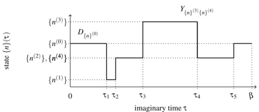
In this chapter we will present a different approach—the configuration path integral Monte Carlo (CPIMC) method [23]. The main idea of this approach is to evaluate the path integral not in configuration space (as in DPIMC), but in second quantization. This leads to paths in Slater determinant space in occupation number representation instead of paths in coordinate space. The idea is based on the continuous time path integral method [24, 25], which is widely used for lattice models such

(3)

as the Hubbard model, see [26], and for impurity models, see [27]. These models are described by simplified Hamiltonians where the interaction is typically of short- range. However, for many systems, in particular plasmas, the long-range Coulomb interaction is of central importance. In this chapter we will show how the CPIMC idea can be used to calculate thermodynamic properties of plasmas or, more generally, spatially continuous fermionic systems with arbitrary pair interactions.

The chapter will start with a short introduction to Metropolis Monte Carlo methods and an advanced description of the estimation of statistical errors. We will then introduce the formalism of the second quantization as far it is needed to understand the presented algorithm and give a short overview over the equations of statistical quantum physics that describe the thermodynamics of the systems of interest in equilibrium. In the main part we will derive the underlying formulas of CPIMC in detail and give a complete description of the MC algorithm. At the end of the chapter a demonstrative application of the method to a one-dimensional system of Coulomb-interacting fermions in a harmonic trap will be discussed.

2 Monte Carlo

In the first section of this chapter, theMetropolis algorithm, which has been developed by Metropolis et. al.in 1953 [28], shall be explained in a fairly general form. The next section, where we will briefly illustrate how to estimate the error of quantities computed with theMetropolis algorithm, is based on [29]. We mention that similar Monte Carlo methods are used also in the chapters by Thomsen et al.

(classical Metropolis MC) and Rosenthal et al. (kinetic MC) of this book.

2.1 Metropolis algorithm

Our ultimate goal is the computation of thermodynamic properties of quantum many-body systems in equilibrium. However, the following considerations are completely general and are valid for classical and quantum systems. In the classical case, we only have to remove the operator heats of the observables. Regardless of the chosen ensemble, expectation values of observables ˆOare always of the form

hOˆi= Z

∑

C

O(C)W(C)

Z with Z=

Z

∑

C

W(C). (1)

The partition functionZis given by the sum over all weightsW(C), where the multi- variableCdefines exactly one contribution to the partition function, i.e. one specific weight. Moreover, we refer to the multi-variableCas a configuration or a microstate of the system. Such a configuration is generally defined by a set of discrete and/or

(4)

continuous variables, which is why the symbol Z

∑

C

was introduced in (1) denoting the integration or summation over all these variables. Further, O(C) denotes the value of the observable in the configurationC. We can interpretP(C) =^W^(C)_Z as the probability of the system to be in the configurationCif and only if the weightsW(C) are always real and positive. Hence, the expectation value of an observable [Eq. (1)]

is given by the sum over all possible values of the observableO(C)weighted with its corresponding probability.

The difference between classical and quantum systems as well as the choice of the ensemble (microcanonical, canonical or grand canonical ensemble) enter in the actual form of the weights and in the set of variables necessary to define a configuration. [In Chap. 1 by Thomsen et al., Metropolis Monte Carlo of a classical system in the canonical ensemble is described.] For a quantum system, the partition function is given by the trace over theN−particle density operator ˆρ discussed in detail in Sec. 4 below:

Z=Tr ˆρ. (2)

Each choice of a different basis in which the trace is performed leads to a different Monte Carlo algorithm. For example, performing the trace in coordinate space results in the DPIMC method [12], whereas the occupation number representation yields the CPIMC method described in Sec. 5 and [23].

Now we will continue with the general consideration of theMetropolis algorithm for quantum and classical systems. Using theMetropolis algorithm, one can generate a sequence of configurationsC_i which are distributed with probabilityP(Ci).

However,P(Ci)involves the partition functionZ(normalization of the distribution), that is typically very hard to compute. To avoid this problem, one defines a transition probabilityv(C_i→C_i+1)for the system that characterizes the transition into the con- figurationC_i+1starting fromCi. To ensure that the configurationsCiare distributed withP(Ci), the transition probability has to fulfill thedetailed balance condition¹:

P(Ci)v(Ci→C_i+1) =P(Ci+1)v(Ci+1→C_i). (3) A possible solution of this equation is given by

v(Ci→C_i+1) =min

1,P(Ci+1) P(Ci)

=min

1,W(Ci+1) W(Ci)

. (4)

Now the algorithm works as follows. Suppose the system is in the configurationC_i. A Monte Carlo step then consists of proposing a certain change of the configuration converting it intoC_i+1. After that, a random number from[0,1)is generated, and the transition probability is calculated according to Eq. (4). If the random number is smaller thanv(Ci→C_i+1), then the change (Monte Carlo step) is accepted. Oth- erwise, the system stays in the previous configuration, i.e. it isC_i+1=C_i. Starting

1In fact, there are weaker conditions on the transition probabilities, but in practice, one uses the detailed balance.

(5)

from an arbitrary configurationC₀, after some steps, the configurations will be distributed withP(C)forming a so-calledMarkov chain. We refer to the number of steps which are necessary for the initial correlations to vanish as theequilibration time.

In addition to thedetailed balance, we have to make sure the transition probabilities are ergodic, i.e. it must be possible to reach every configuration withW(C)>0 in a finite number of steps. In practice, one will usually need a few different Monte Carlo steps to ensure the ergodicity. These steps address different degrees of freedom of the configurations, which, of course, depend on the actual form of the partition function, Eq. (1). Furthermore, in the majority of cases, it will be more efficient not to propose every change of the configuration with equal probability. Therefore, we split the transition probability into a sampling probabilityT(Ci→C_i+1)and an acceptance probabilityA(Ci→C_i+1)for that specific change, i.e. it is

v(Ci→C_i+1) =A(Ci→C_i+1)T(Ci→C_i+1). (5) Inserting this factorization into thedetailed balance, one readily obtains the solution for the acceptance probability

A(Ci→Ci+1) =min

"

1,T(Ci+1→C_i)W(Ci+1) T(Ci→C_i+1)W(Ci)

#

. (6)

This generalization is also called theMetropolis Hastings algorithm. The algorithm is most efficient if the acceptance probability is about 50%. A suitable choice of the sampling probability can help optimizing the acceptance probability.

Once we have generated aMarkov chainof lengthN_MCvia theMetropolis algorithm, a good estimator for the expectation value of an observable is given by

hOˆi ≈ 1 N_MC

NMC

i=1

∑

O(Ci) =:O, (7)

which directly follows from Eq. (1) and the fact that all configurationsCi in the Markov chainare distributed withP(Ci).

Unfortunately, the weightW(C)is not always strictly positive, so we can not always interpret ^W(C)_Z as a probability. Especially for systems of fermions, there are many sources of sign changes in the weights. However, we can still apply the Metropolis algorithmif we define a new partition function

Z⁰:=

∑

C

|W(C)|, (8)

and rewrite the expectation values as follows:

hOˆi=∑CO(C)W(C)

∑CW(C) =

1

Z⁰∑CO(C)S(C)|W(C)|

1

Z⁰∑CS(C)|W(C)| =hOSˆ i⁰

hSi⁰ , (9)

(6)

whereS(C) =sgn[W(C)]denotes the sign of the weight. Obviously, the expectation value of ˆOin the physical system, described by the partition functionZ, is equivalent to the expectation value of ˆOSdivided by the expectation value of the sign (average sign), both averaged in the primed system described by Z⁰, cf. Eq. (8). For that system, we can generate aMarkov chainif we simply insert the modulus of the weights|W(C)|in Eq. (6) when computing the acceptance probability. Combining Eq. (7) and (9), we obtain an expression for the estimator of the observable in the real system:

hOˆi ≈∑^N_i=1^MCO(C_i)S(C_i)

∑^N_i=01^MCS(Ci) =:OS⁰

S⁰ =O. (10)

Thus, we actually simulate the primed system and calculate quantities of the physical system via Eq. (10).

2.2 Error in the Monte Carlo simulation

Estimating the errors of quantities computed with theMetropolis algorithmis not a trivial task. First, we consider the case of strictly positive weights, where the estimator of an observable is given by Eq. (7). It is reasonable to interpret the values of the observable in each configuration of theMarkov chainas a series of measurements.

The estimatorO, which is obtained by averaging over all measurements, fluctuates statistically around the true expectation valuehOˆi. The error of the arithmetic mean of a measurement series of lengthN_MCis defined by

∆O= σ_O

√N_MC , (11)

whereσ_O is the standard deviation which, for uncorrelated measurements, can be estimated by

σ_O= v u u t 1

(NMC−1)

N_MC i=0

∑

(Oi−O)², with O_i=O(Ci). (12) Certainly, the “measurement” series obtained from theMarkov chainis correlated, since we generate each configuration from the previous one. The correlation of these configurations can be measured by the integrated auto-correlation time

τ_int,O=1 2+

N_MC k=1

∑

O_iO_i+k−O²

σ_O²_¯ , (13) with OiO_i+k= 1

N_MC

N_MC i=1

∑

OiO_i+k.

(7)

The auto-correlation of the measurements enhances the statistical error by a factor ofp

2τ_int,O, i.e. it is

∆O_auto=∆Op

2τ_int,O=√σO¯

N_MC

p2τ_int,O=√σO¯

N_eff. (14) Therefore, if we have generated aMarkov-chainof lengthN_MC, we have effectively gained only _2τ^N^MC

int,O uncorrelated measurements. To keep the correlation small, efficient Monte Carlo steps are essential, which change many degrees of freedom of the configurations simultaneously while still having an acceptance ratio of about 50%. In practice, acceptance ratios are much smaller than 50%, and one therefore performs a certain number of Monte Carlo steps (acycle) before again measuring the observables.

Things become more complex if the weights are not strictly positive. In that case, we have expressed quantities of the physical system by quantities of the primed system, Eq. (10). We simulate the primed system and calculate the r.h.s. of Eq. (10) to obtain O. The measurements of the quantities OS⁰ and S⁰ are not only auto- correlated but also cross-correlated with each other. The relative statistical error can be estimated according to (cf. [29])

∆O_auto,cross

O =

v u u t ∆OS⁰

OS⁰

!2

+ ∆S⁰ S⁰

!2

− 2 N_MC

OSS⁰−OS⁰S⁰ OS⁰S⁰

2τ_int,OS,S, (15)

where we have the statistical errors ofOS⁰andS⁰

∆OS⁰= s

(OS)²⁰−(OS)⁰²

N_MC 2τ_int,OS,

∆S⁰= s

S²⁰−S⁰²

N_MC 2τ_int,S, (16)

each enhanced by their individual auto-correlation time and in the last term the integrated cross-correlation time

τint,OS,S=1 2+

NMC

k=1

∑

O_iS_iS_i+k⁰−OS⁰S⁰

OSS⁰−OS⁰S⁰ , with O_iS_iS_i+k⁰= 1 N_MC

NMC

i=1

∑

O_iS_iS_i+k. Assuming we are working in the canonical ensemble, then, from the definition of the partition function and theaverage sign, cf. Eq. (9), it immediately follows that

S⁰≈ hSi⁰= Z

Z⁰ =e⁻^β^N(^f⁻^f⁰⁾≤1, (17) whereβ is the inverse temperature,Nthe particle number, and f⁽⁰⁾the free energy per particle in the physical (primed) system. Combining Eqs. (15) and (17) yields

(8)

∆O_auto,sign

O ∝ 1

S⁰√

N_MC ≈ 1

√N_MCe^βN(^f⁻^f⁰⁾. (18) The relative error of an observable grows exponentially with the product of the particle number, the inverse temperature and the difference of the free energy per particle in the physical and the primed system. Unfortunately, the error can only be reduced with the square root of the number of Monte Carlo samples (measurements). There- fore, the value of theaverage signof a given system determines if one can compute reliable quantities via theMetropolis algorithmfor that system. This severe limita- tion is called the (fermion)sign problem. In practice, an average sign of the order

≈10⁻³is the limit for reliable Monte Carlo simulations. Also, one should be aware that even the sign itself has a statistical error of the form (14). Besides, we note that the proportionality (17) can be obtained by a simple Gaussian error propagation of O, cf. Eq. (10).

Thesign problemis strongly dependent on the actual representation of the partition function, cf. Eq. (1). For some special systems, thesign problemcan be cir- cumvented by a specific choice of the representation [30, 31], but a general solution is highly unlikely, since it has been shown to be NP-complete [15].

3 Second quantization

Second quantization refers to the introduction of creation and annihilation operators for the description of quantum many-particle systems. Thereby, not only the observables are represented by operators but also the wave functions, in contrast to the standard formulation of quantum mechanics (correspondingly called “first”

quantization), where only the observables are represented by operators. The proper symmetry properties of the bosonic (fermionic) many-particle states are automatically included in the (anti-)commutation relations of the creation and annihilation operators. Simultaneously, also observables can be expressed by these operators.

This unifying picture of quantum mechanics is often advantageous when it comes to the description of many-particle systems.

Since CPIMC makes extensive use of the second quantization of quantum mechanics, a brief introduction will be given in this section, where we will focus on those aspects which are necessary for the comprehension of the method. Especially the derivation of the crucialSlater-Condon rulesshall be outlined. For a detailed introduction to the second quantization see e.g. [32].

3.1 (Anti-)Symmetric many-particle states

We consider a system ofNidentical, ideal (i.e. not interacting) quantum particles which is described by the Hamiltonian ˆH₀. For an ideal system, the Hamiltonian can

(9)

be written as a sum of one-particle Hamiltonians:

Hˆ₀=

N α=1

∑

hˆ_α, (19)

hˆ_α= pˆ²_α

2m+vˆ_α, (20)

where ˆp_α denotes the momentum operator and ˆv_α the operator of the potential energy of the particleα in an external field. Thus, the subscriptα indicates that those operators are acting on states from the one-particle Hilbert spaceHαof the particle α. We imply that the solutions of the eigenvalue problem

hˆ|ii=ε_i|ii, with i∈N₀ (21) are known. The one-particle states|iiform a complete orthonormal system (CONS) of the one-particle Hilbert space. Further, we assume the states are arranged according to their one-particle energy, i.e.εi≤εjfor alli≤j. In general, the one-particle states are spin orbitals, i.e.|ii ∈Hcoord⊗Hspin with the tensor product of the coordinate and spin Hilbert space. Hence, the wave functionhrσ|ii= (hr|hσ|)|ii= φi(r,σ)depends on both the coordinaterand the spin projectionσ of the particle.

In the case of an ideal system, the solution of theN−particle eigenvalue problem

Hˆ₀|Ψi=E|Ψi (22)

can be constructed from products of one-particle states:

|i₁i₂. . .iNi=|i₁i1|i₂i2. . .|i_NiN . (23) The many-body Hilbert space ofNparticlesH^N =^N^N_α=1Hα is thus given by the tensor product of one-particle Hilbert spaces. The states|i₁i₂. . .iNiform a basis of H^N, and the used notation indicates that particleαis in the state|i_αi.

Apart from some special exceptions as e.g. Axions, only totally symmetric or antisymmetric states with respect to arbitrary two-particle exchanges are physically realized, i.e. states with

|. . .iα. . .i_β. . .i_±=±|. . .i_β. . .iα. . .i ∀α,β . (24) Particles that are described by symmetric states (upper sign) are called bosons and those with antisymmetric states (lower sign) fermions. The reason for this symmetry ofN−particle states lies in the indistinguishability of the quantum particles, whereby physical properties of the system cannot change under particle exchange.

The spin-statistics-theorem states that fermions have half-integer and bosons integer spin.

Totally (anti-)symmetric states can be constructed from the product states (23) by summing up allN! permutations ofNparticles:

(10)

|i₁i₂. . .iNi_±= 1 N

∑

P∈S_N

(±1)^PPˆ|i₁i1|i₂i2. . .|i_NiN , (25)

wherePˆ is theN−particle permutation operator that can be constructed from a composition of two-particle exchanges. The normalization factorN is given by

N =







pN!∏^∞_i=0n_i, for bosons,

√N!, for fermions,

(26)

wheren_idenotes the number of one-particle states|iiin the product state. The hermitian operator ˆS(A)ˆ

S/ˆ Aˆ= 1 N

∑

P∈SN

(±1)^PPˆ, (27) is referred to as the (anti-)symmetrization operator. For fermions, the sign of each summand is determined by the number of two-particle exchangesPin the permutation operator ˆP. Further, arbitrary (anti-)symmetric states can be constructed from linear combinations of these (anti-)symmetric states, Eq. (25). Therefore, they form a basis in the (anti-)symmetric Hilbert spaceH_±^N⊂H^N. The operator(N /N!)Sôr (N /N!)Aîs a projection operator on the respective subspace, it is ˆS²= (N!/N)Sˆ and Â²= (N!/N )A, respectively and also ˆˆ SAˆ=0.

In coordinate-spin representation, the anti-symmetric product states of fermions can be written as determinants (calledSlater determinants):

Ψ(x1, . . . ,x_N)₋= 1 N!

φi₁(x1) φi₂(x1)··· φi_N(x1) φi₁(x2) φi₂(x2)··· φi_N(x2)

... ... ... φi1(xN)φi2(xN)···φiN(xN)

. (28)

For bosons, one obtains instead permanents. From this representation of antisymmetric states it becomes obvious that there is none with a one-particle state occurring twice in the product state, for a determinant with two equal columns vanishes. This is also known as the famousPauli principle. For bosons, there is no such restriction.

3.2 Occupation number representation

Due to the (anti-)symmetrization of the many-particle states (25), such states are entirely characterized by the occurrence frequency of each one-particle state in the product state. The number of particlesn_i in the one-particle state|iiis called the occupation number (of thei-th state/orbital). Since the complete set of occupation numbers, denoted with{n}, defines an (anti-)symmetric many-particle state, we can

(11)

also write

|i1. . .i_Ni_±≡ |n0n1n2. . .i=:|{n}i, (29)

with

n_i∈ (

N0 , for bosons {0,1} , for fermions .

The order of the occupation numbers equals the order of the one-particle states in the product state, which can be arbitrary but must remain fixed for further calculations.

ThePauli principlefor fermions is automatically included in the restriction on the occupation numbers to be either zero or one.

If we only consider many-particle states with fixed particle number,N=∑^∞_i=0n_i, then the states|{n}iform a CONS of the (anti-)symmetricN−particle Hilbert space N_±^Nwith the orthogonality relation

h{n}|{n¯}i=

∞

∏

i=0

δni,n¯i=:δ_{_n_}_,_{_n_¯_}, (30) and the completeness relation

∑

{n}

|{n}ih{n}|δ_∑_i_n_i_,N =ˆ1N. (31) To shorten the notation, we introduced the following abbreviation:

∑

{n}

:=







∑^∞_n₀₌₀∑^∞_n₁₌₀···, for bosons

∑¹_n₀₌₀∑¹_n₁₌₀···, for fermions

. (32)

In practical simulations, one has to work with a finite number of one-particle orbitals N_B. This equals the approximation

∑

{n}

≈







∑^∞_n₀₌₀∑^∞_n₁₌₀···∑^∞_n_NB₌₀, for bosons

∑¹_n₀₌₀∑¹_n₁₌₀···∑¹_n_NB₌₀, for fermions

. (33)

Given a certain one-particle basis, each antisymmetric state|{n}ican be uniquely identified with aSlater determinant(28). The relations (30) and (31) are consistent with the respective relations for determinants. For that reason, it is common to also refer to the states|{n}iasSlater determinants.

Now we drop the restriction of a fixed number of particles. The inner product in Eq. (30) is still well defined for states with different particle numbers; only the completeness relation is slightly modified

(12)

{n}

∑

|{n}ih{n}|=ˆ1. (34)

The states |{n}ithereby form a CONS in the so-called Fock spaceF_±=H⁰⊕

H¹⊕H_±². . ., which contains (anti-)symmetric states of varying particle number.

Consequently, any state of the Fock space can be written as a linear combination of theSlater determinants|{n}i:

|Ψi=

∑

{n}

c_{_n_}|{n}i . (35)

For example, if we consider a general Hamiltonian of interacting particles

Hˆ=Hˆ₀+Wˆ , (36)

where we added the interaction operator ˆW to the ideal Hamiltonian ˆH₀, then the solution|Ψiof the eigenvalue problem

Hˆ|Ψi=E|Ψi, (37)

can in general not be written in terms of a singleSlater determinant|{n}ibut will be of the form (35). Besides, those states do not necessarily have a defined particle number. Furthermore, theSlater determinantwithout any particles|00. . .i=|{0}i is thevacuum statethat is normalized to one according to Eq. (30) and also belongs to the Fock space (Thevacuum stateshould not be confused with the zero vector).

Finally, we could have chosen any arbitrary, complete one-particle set{|νi}in the definition of the states|{n}i, cf. Eq. (29). Since from the states|{n}iit is not clear which one-particle basis has been used for the quantization, one usually has to explicitly specify the chosen basis.

3.3 Creation and annihilation operators

The introduction of creation and annihilation operators, which induce transitions between states of different particle number, is of crucial importance for the formalism of the second quantization. Originally, these operators have been constructed for the description of the harmonic oscillator (so-called ladder operators). In the following bosons and fermions will be treated separately.

3.3.1 Bosons

In the bosonic case, the action of the creation and annihilation operators on symmetric states in the occupation number representation is defined by

(13)

ˆ

a^†_i|n₀n₁. . .ni. . .i=p

n_i+1|n₀n₁. . .n_i+1. . .i, (38)

ˆ

a_i|n₀n₁. . .ni. . .i=√n_i|n₀n₁. . .ni−1. . .i, (39) where the prefactors ensure the correct normalization. Apparently, the annihilation operator vanishes forn_i=0. Hence, the creation and annihilation operators are not hermitian but pairwise adjoint. The bosonic creation and annihilation operators fulfill the commutation relations

[aˆ^†_i,aˆ^†_j] = [aˆ_i,aˆ_j] =0,

[aˆ_i,aˆ^†_j] =δ_i,_j, (40) with the commutator[A,ˆ B] =ˆ AˆBˆ−BˆA. Using the creation operator, we can constructˆ arbitrary states of the form (29):

|{n}i= 1

√∏in_i! ^∞

∏

i=0

(aˆ^†_i)ⁿⁱ

|{0}i. (41)

Of particular interest is the hermitian occupation number operator of thei−th orbital ˆ

n_i=aˆ^†_iaˆ_i. (42) Its action is given by

ˆ

n_i|{n}i=n_i|{n}i , (43) and the eigenvalues are simply the occupation numbersn_iof thei−th orbital. Simi- larly, we have the total particle number operator

Nˆ =

∞ i=0

∑

nˆi, (44)

with the total particle numberNof the state as its eigenvalue

Nˆ|{n}i=N|{n}i. (45) Consequently, the states|{n}iare common eigenstates of the occupation number operator, the particle number operator and the ideal Hamilton operator (if we choose the ideal one-particle basis (21) for the quantization).

3.3.2 Fermions

For fermions, the states have to be antisymmetric. A definition of the fermionic creation and annihilation operators which satisfies this condition is given by

(14)

ˆ

a^†_i|{n}i= (1−n_i)(−1)^α^{ⁿ^}^,i|. . . ,ni+1, . . .i, ˆ

a_i|{n}i=n_i(−1)^α^{ⁿ^}^,i|. . . ,ni−1, . . .i, (46)

where the sign is determined by

α_{n},i=

i−1 l=0

∑

n_l. (47)

The sign is positive if the number of particles in the one-particle states before the i−th state is even (with respect to the chosen order) and negative if it is odd. Further, the prefactors ensure that the creation (annihilation) operator vanishes if the orbitali, where the particle shall be created (annihilated), is already occupied (unoccupied), and so the definition also includes thePauli principle. In contrast to the bosonic commutation relations, for fermions, the creation and annihilation operators fulfill the three anti-commutation relations:

{aˆ^†_i,aˆ^†_j}={aˆ_i,aˆ_j}=0,

{aˆ_i,aˆ^†_j}=δi,j (48) with the anti-commutator being defined as{A,ˆ Bˆ}=AˆBˆ+BˆA. When it comes toˆ the algebraic treatment of physical systems, the only difference between the second quantization for bosons and for fermions lies in the difference of the commutation relation (40) and anticommutation relation (48). For example, from the first anticommutation relation directly follows that(aˆ^†_i)²=0, i.e. doubly occupied orbitals do not exist in the case of fermions. As a consequence of the non-commutativity of the fermionic creation and annihilation operators, we have to make sure the ordering of the creation operators equals the chosen order of the orbitals when constructing an arbitrary state from the vacuum states according to

|{n}i=^∞

∏

i=0

(aˆ^†_i)ⁿⁱ

|{0}i. (49)

The formulas for the occupation number operator and the particle number operator (42)-(44) remain unchanged for fermions.

For further calculations, we will need the matrix elements of the creation and annihilation operators

h{n}|aˆ^†_k|{n¯}i= (−1)^α^{ⁿ^}^,kδ_{^k_n_}_,_{_n_¯_}δ_n_k_,1δ_n_k_,¯_n_k₊₁, h{n}|aˆ_k|{n¯}i= (−1)^α^{ⁿ^}^,kδ_{^k_n_}_,_{_n_¯_}δn_k,0δn_k,¯n_k−1,

δ_{^k_n_}_,_{_n_¯_}:=

∞

∏

i=0 i6=k

δ_n_i_,¯_n_i . (50)

(15)

These follow directly from the definitions (46). Evidently, the creation and annihilation operators are defined with respect to a certain one-particle basis{|ii}, the basis that we chose for the quantization. The transformation of the creation and annihilation operators to a different basis{|νi}can be performed as follows:

ˆ a^†_ν=

∞ i=0

∑

hi|νiaˆ^†_i , (51) ˆ

a_ν=

∞ i=0

∑

hν|iiaˆ_i. (52)

For example, choosing spin-coordinate space for the quantization, i.e.|νi=|xi,x= {r,σ}, leads to the so-calledfield operators

Ψˆ^†(x):=aˆ^†_x=

∞

i=0

∑

hi|xiaˆ^†_i =

∞ i=0

∑

φ_i^∗(x)aˆ^†_i, (53) Ψ(x)ˆ :=aˆ_x=

∞

i=0

∑

hx|iiaˆ_i=

∞ i=0

∑

φi(x)aˆ_i. (54) Thefield operatorΨˆ^†(x)creates and ˆΨ(x)annihilates a particle at the space pointr with spin projectionσ.

3.4 Operators in second quantization

Arbitrary first quantized operators can be expressed in the second quantization via the creation and annihilation operators. In the following, we will consider this representation for the one- and two-particle operators. For fermions, in particular, we will give the expressions for the corresponding matrix elements of the interaction potential, which leads to theSlater-Condon-rules.

3.4.1 One-particle operators

Though somewhat misleadingly, it is common to refer to theN−particle operator Bˆ₁=

∑

α

bˆ_α, (55)

that is a sum of true one-particle operators ˆb_α as a “one-particle operator”, too. In second quantization, that operator takes the following form:

Bˆ₁=

∞ i,j=1

∑

b_{i j}aˆ^†_iaˆ_j, (56)

(16)

with the one-particle integrals b_{i j}=hi|bˆ|ji=

Z

dxφ_i^∗(x)b(x)φj(x), (57) where the integration overx={r,σ}includes an integration over the space coordinate and a summation over the spin. As usual, we have assumed local operators in coordinate space. From the matrix elements of the creation and annihilation operators (50), we readily obtain the matrix elements of the one-particle operators (56):

h{n}|aˆ^†_laˆ_k|{n¯}i=

∑

{n0}

h{n}|aˆ^†_l|{n⁰}ih{n⁰}|aˆ_k|{n¯}i

=

∑

{n⁰}

(−1)^α^{ⁿ^0}^,l^+α^{ⁿ^¯^},kδ_{^l_n_}_,_{_n₀_}δ_{^k_n₀_}_,_{_n_¯_}δ_n0

l,0δ_n_l_,1δ_n_¯_k_,1δ_n0

k,0. (58)

Via case differentiation we can simplify this to h{n}|aˆ^†_laˆ_k|{n¯}i=

((−1)^α^{ⁿ^}^,l^+α^{ⁿ^¯^}^,kδ_{^kl_n_}_,_{_n_¯_}δ_n_l_,1δ_n_¯_k_,1δ_n_¯_l_,0δ_n_k_,0, k6=l

n_lδ_{_n_}_,_{_n_¯_}, k=l . (59) Inserting this into Eq. (56) and rearranging the sums with respect to terms withk=l andk6=lyields

h{n}|Bˆ₁|{n¯}i=δ_{_n_},{_n_¯_}

∞ k=0

∑

b_kkn_k

+

∞ k=1

∑

∞ l=1

∑

l6=k

b_lk(−1)^α^{ⁿ^}^,l^+α^{ⁿ^¯^}^,kδ_{^kl_n_}_,_{_n_¯_}δ_n_l_,1δ_n_¯_k_,1δ_n_¯_l_,0δ_n_k_,0. (60)

The first term only gives a contribution if bothSlater determinantsare equal; thus, these are the diagonal elements of the matrix. The second term does not vanish only if the right and left state differ in exactly two occupation numbers while conserving the total particle number.

Let|{n}q^pibe theN−particle state that one obtains from the state|{n}iif one particle is removed from theq−th orbital and added to the p−th orbital, i.e. for q<pit is

|{n}q^pi=|. . . ,nq−1, . . . ,np+1, . . .i. (61)

Using this notation, we can rewrite the matrix elements of a one-particle operator of the form (56) in a compact way:

(17)

h{n}|Bˆ₁|{n¯}i=











∞ k=1∑

b_kkn_k, {n}={n¯} b_pq(−1)

max(p,q)−1

∑

l=min(p,q)+1

n_l

, {n}={n¯}q^p

0, else

. (62)

Thereby, we have expressed the matrix elements of a second quantized one-particle operator (56) by the one-particle integrals (57).

3.4.2 Two-particle operators

In analogy to the one-particle operators, general two-particle operators of the form Bˆ₂=¹₂∑^N_α₆_=β=1bˆ_α,β take the following form in second quantization:

Bˆ2=1 2

∞ i,j,k,l=1

∑

b_{i jkl}aˆ^†_iaˆ^†_jaˆ_laˆ_k. (63) Note the exchange of the orbital indices of the annihilation operators and the two- particle integrals, which is important for fermions due to the non-commutativity of the creation and annihilation operators. The two-particle integrals are given by

b_{i jkl}=hi j|bˆ|kli= Z

dx Z

dyφ_i^∗(x)φ^∗_j(y)b(x,y)φk(x)φl(y). (64) The following considerations are restricted to fermions only. For the most interesting case of the pair interaction operator ˆW, one can take advantage of the fact that the interaction is symmetric under particle exchange, i.e.w(x,y) =w(y,x), and real, i.e.

w^∗(x,y) =w(x,y). Hence, for the two-particle integrals, we have

w_{i jkl}=w_jilk, (65)

w^∗_{i jkl}=w_{kli j}. (66)

Using these symmetries, we can bring the interaction operator into a more suitable form:

Wˆ =

∞ i=1

∑

∞ j=i+1

∑

∞ k=1

∑

∞ l=k+1

∑

w⁻_{i jkl}aˆ^†_iaˆ^†_jaˆ_laˆ_k, (67) where we have introduced the antisymmetric two-particle integralsw⁻_{i jkl} =w_{i jkl}− w_{i jlk}. Obviously, there are only terms withi< jandk<l. Therefore, we end up with six different cases to be considered:

(18)

Wˆ =

∑

i=1

∑

j=i+1

w⁻_{i ji j}aˆ^†_jaˆ^†_iaˆ_iaˆ_j+

∑

i=1

∑

j=i+1

∑

l=i+1 l6=j

w⁻_{i jil}aˆ^†_jaˆ^†_iaˆ_iaˆ_l

+

∑

i=1

∑

j=i+1 j−1 k=1

∑

k6=i

w⁻_{i jk j}aˆ^†_jaˆ^†_iaˆ_kaˆ_j+

∑

i=1

∑

j=i+1 i−1 k=1

∑

w⁻_{i jki}aˆ^†_jaˆ^†_iaˆ_kaˆ_i +

∑

i=1

∑

j=i+1

∑

l=j+1

w⁻_{i j jl}aˆ^†_jaˆ^†_iaˆ_jaˆ_l+

∑

i=1

∑

j=i+1

∑

kk=16=i,j l=k+1

∑

l6=i,j

w⁻_{i jkl}aˆ^†_jaˆ^†_iaˆ_kaˆ_l. (68)

For each of these cases, one readily computes the matrix elementsh{n}|aˆ^†_jaˆ^†_iaˆ_kaˆ_l|{n¯}i. Rearranging of the terms finally yields

h{n}|Wˆ|{n¯}i= δ_{_n_}_,_{_n_¯_}

∞ i=1

∑

∞ j=i+1

∑

w⁻_{i ji j}n_in_j

+

∞ p=1

∑

∞ q=1

∑

δ_{^pq_n_},{_n_¯_}δnp,1δn¯p,0δnq,0δn¯q,1

·

∞ i=1

∑

w⁻_ipiq(−1)^α^{ⁿ^}^,i^+α^{ⁿ^¯^}^,i^+α^{ⁿ^}^,p^+α^{ⁿ^¯^}^,qΘ(i,p,q)ni

+

∞ p=1

∑

∞ q=p+1

∑

∞ r=1

∑

∞ s=r+1

∑

δ_{^pqrs_n_},{_n_¯_}δnp,1δn¯p,0δnq,1δn¯q,0δnr,0δn¯r,1δns,0δn¯s,1

·w⁻_pqrs(−1)^α^{ⁿ^}^,p^+α^{ⁿ^}^,q^+α^{ⁿ^¯^}^,r^+α^{ⁿ^¯^}^,s ,

(69) with

Θ(i,p,q) =







−1, p<i<q, or q<i<p 0, i=p or i=q

1, else

. (70)

Thus, there are three different contributions to the matrix elements. These are the Slater-Condon-rules[32], which can be rewritten as follows:

(19)

Wˆ_{_n_},{_n_¯_}:=h{n}|Wˆ|{n¯}i=Wˆ_{Î_n_}_,_{_n_¯_}+Wˆ_{ÎI_n_}_,_{_n_¯_}+Wˆ_{ÎII_n_}_,_{_n_¯_}, Wˆ_{Î_n_}_,_{_n_¯_}=δ_{n},{_n}_¯

∞ i=0

∑

∞ j=i+1

∑

w⁻_{i ji j}n_in_j, Wˆ_{^II_n_}_,_{_n_¯_}=

∞ p,q=1

∑

δ_{^pq_n_}_,_{_n_¯_}δ_n_p_,1δ_n_¯_p_,0δ_n_q_,0δ_n_¯_q_,1

∑

i6=p,qi=0

w⁻_ipiq(−1)^∑^max(p,q)−

1 l=min(p,q)+1n_l

n_i,

Wˆ_{^III_n_}_,_{_n_¯_}=

∞ p=1

∑

∞ q=p+1

∑

∞ r=1

∑

∞ s=r+1

∑

δ_{^pqrs_n_}_,_{_n_¯_}δnp,1δn¯p,0δnq,1δn¯q,0δnr,0δn¯r,1δns,0δn¯s,1

·w⁻_pqrs(−1)^∑^q⁻

1

l=pn_l+∑^s_l=r⁻¹n¯_l

.

(71)

The first term only gives a contribution if both states are equal and the second if left and right state differ in exactly two orbitals. In contrast, the third term is not vanishing only if both states differ in exactly four orbitals. In all cases, the left and right state must have the same particle number. All other matrix elements vanish.

Collecting the obtained results, we finally end up with

h{n}|Wˆ|{n¯}i=











∑^∞_i=0

∞

∑

j=i+1

w⁻_{i ji j}n_in_j, {n}={n¯}

∑i=0

i6=p,qw⁻_ipiq(−1)^∑

max(p,q)−1 l=min(p,q)+1nl

ni, {n}={n¯}^pq

w⁻_pqrs(−1)^∑^q⁻

1

l=pn_l+∑^s_l=r⁻¹n¯_l

, {n}={n¯}^p<qr<s

0, else

. (72)

Thereby,|{n}r<s^p<qiis theN−particle state that one obtains from|{n}iif a particle is added to the orbitals|piand|qieach, withp<q, and removed from the orbitals|ri and|si, withr<s.

4 The density operator

The density operator ˆρ is of extreme importance for the description of thermodynamic properties of quantum many-particle systems. While in standard quantum mechanics a quantum system is described by a certain state|Ψi, this does not apply to a quantum system at a finite temperature (e.g. a system in a thermostate). In this case, in principle, all possible states may be observed with a certain probability, i.e.

the system is in an ensemble of states or in a “mixed state”. For an ensemble of possible many-particle states{|Ψii}, the density operator (which replaces the wave function in the previous case of a “pure” state) is defined as

ρˆ=

∑

i

P(|Ψii)|ΨiihΨi|. (73)

(20)

The sum goes over all states of the ensemble, andP(|Ψ_ii)is the real, positive probability to observe the state|Ψ_ii. The matrix representation of ˆρ in an arbitrary N- particle basis{|Φ_ii}is called the density matrixhΦ|ρˆ|Φi. Further, it is hermitian, i.e. ˆρ^†=ρ, and positive semi-definite, i.e.ˆ hΦi|ρˆ|Φii ≥0 for arbitrary states|Φii. The probabilities obey the normalization∑iP(|Ψii) =1, which corresponds to

Tr ˆρ=

∑

i

hΦi|ρˆ|Φii=1, (74) where the trace can be evaluated in an arbitrary N-particle basis. The most important feature of the density matrix is that we can compute the expectation value of any observable via

hOˆi=Tr(Oˆρ)ˆ . (75) It is always Tr ˆρ²≤1, and for a mixed ensemble this expression is strictly smaller than 1. For a pure state |Ψi, the density operator becomes a projection operator with ˆρ²=ρˆ and (75) turns into the standard quantum mechanical averagehOˆi= hΨ|Oˆ|Ψi. The entropy of the system can be defined as

S=−hln ˆρi. (76)

Hence, the density operator contains the whole thermodynamic information of the system.

In the canonical ensemble, characterized by the particle numberN, the tempera- tureT and the volumeV of the system, the density operator takes the form

ρˆ(N,β,V) = 1

Z(N,β,V)e⁻^β^H^ˆ, (77) with the inverse temperatureβ=_T¹ (we usek_B=1). The normalization factorZis the partition function

Z(N,β,V) =Tre⁻^β^H^ˆ. (78) For most of the physical quantities, the whole information about theN-particle density operator is not required. Instead, it is sufficient to know the partition function.

Another crucial quantity of the canonical ensemble is the free energy

F(N,β,V) =−TlnZ. (79) Most of the physical quantities can also be derived from the free energy, e.g. for the total energy and the heat capacity at constant volume we have

hHˆi=−T² ∂

∂T F T _N,V

=− ∂

∂ β lnZ _N,V

, (80)