A Study of Track Segments within Hadronic Showers with a Highly Granular Hadronic Calorimeter

Hadronic Showers with a Highly Granular Hadronic Calorimeter

Diploma Thesis of Lars Weuste

Ludwig-Maximilians-Universität Department of Physics

Max-Planck-Institut für Physik

Supervisor: Prof. Christian Kiesling

September 7, 2009

Introduction

1 Physics motivation

1.1 The Particle Zoo and elementary particles . . . . 4

1.2 The Standard Model (SM) . . . . 8

1.3 Beyond the Standard Model . . . 11

2 The ILC Detector and CALICE 2.1 The International Linear Collider . . . 13

2.2 The International Large Detector (ILD) . . . 16

2.3 CALICE. . . 27

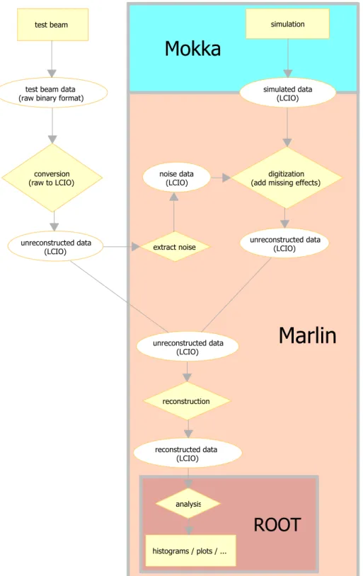
3 Software and Analysis Toolchain 3.1 Analysis Toolchain . . . 38

3.2 Mokka/Geant4: Monte Carlo simulation. . . 40

3.3 Software. . . 43

4 Tracking in hadronic showers 4.1 Motivation. . . 46

4.2 Isolated hits and Track parameters . . . 48

4.3 Tracking via “Follow-Your-Nose” tracking . . . 50

4.4 Tracking via Parameter Search inspired by Hough Transformation . . 56

4.5 Comparison of FYN and Hough inspired Parameter Search . . . 63

4.6 Corrections and Clean Up. . . 67

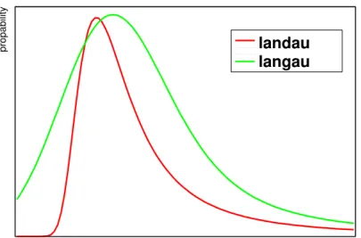
4.7 Determination of the langau peak . . . 71

4.8 Implementation. . . 73

5 Applications 5.1 Track length of primary pions . . . 75

5.2 Temperature Monitoring . . . 77

5.3 Calibration Transportation . . . 78

5.4 Comparison of Monte Carlo to real data. . . 83

6 Conclusion

i

A Tracking Algorithm comparison: CPU and mem- ory performance

B Implementation

B.1 Implementation of tracking algorithms. . . 95 B.2 Analysis Processor. . . 95

Figures. . . 96

With the Large Hadron Collider (LHC, [1]) installed in CERN [2] it will be possible to search for the “missing” Higgs particle and for new physics beyond the Standard Model, such as Super Symmetric Particles. To distinguish the different physical final states a very high precision is necessary. The LHC is a proton - proton collider and hence it is capable of finding new physics at mass scales up to several TeV. Once indications for new physics are found, accurate measurements need to be done with an electron-positron machine. This situation is similar to thespps¯ where the heavy weak bosons were found, and LEP, where the Standard Model was verified with high precision.

The International Linear Collider (ILC) will usee⁺e⁻ instead of protons. There- fore it will have much cleaner events and can provide the needed accuracy with carefully designed detectors. And unlike a hadron detector it has a fixed center of mass energy for the particles in the initial state, which largely improves the pos- sibility to fully reconstruct the final state. However, acquiring and maintaining detectors with required precision is not an easy task. Especially the jet energy resolution has to be much better than with previous detectors. Several detector concepts exist to achieve this. Two of them make use of the particle flow algo- rithm which measures the particles in the subdetector that is suited best for that purpose. Therefore it is necessary to be able to follow the path of single particles even into the calorimeters so that one can assign the measured energy to specific particles. This is only possible in so called imaging calorimeters which feature unprecedented spacial resolution.

Calorimeters are designed to force the incident particles into a shower, depositing all of its energy so it can be measured. This can be done for particles interacting electromagnetically (electron, photon) and for particles that interact hadronically (hadrons). Often sampling calorimeters are used, i.e. in addition to the sensitive material a second, passive material, in which the showering of particles proceed is included, where layers of both materials alternate. This is done to keep the size and therefore the cost of such calorimeters manageable. The calorimeters of the International Large Detector (ILD) are highly granular detectors. For the hadronic part it is planned to have tiles of a size of 30×30×5 mm³ resulting in approximately eight million channels [3]. Each of these tiles is read out by a Silicon Photo Multiplier (SiPM). This raises the problem of establishing a precise inter-calibration of these many channels.

1

The CALICE (CALorimeter forLInear Collider Experiment) collaboration was formed to study electromagnetic and hadronic designs suitable for particle flow calorimetry at the ILC. For this purpose several prototypes where assembled and tested at various accelerator sites in the past few years. The hadronic calorimeter tested in great detail is the analog hadron calorimeter (AHCal). This type of calorimeter is meant as a prototype for the ILD detector. It uses scintillator tiles with a size of 3×3 cm² to 12×12 cm² as sensitive material read out via SiPMs.

With such high resolution ("imaging") hadronic calorimeter built by the CAL- ICE collaboration, it is possible to identify single particle tracks within hadronic showers. Assuming that all particles flying through the detector are minimum ionizing, we then expect the resulting distribution to look like a Landau distri- bution. This peak of the Landau distribution (most probable energy deposition) can be used for cell to cell intercalibration as well as for monitoring the detector performance and stability using real event data.

This diploma thesis will use as small subset of the collected testbeam data from CALICE for developing a tracking algorithm in the hadronic calorimeter to iden- tify single particle tracks. Two options are considered: A simple “follow your nose”

algorithm which uses the last found point as a reference and searches in the direct vicinity for another one to continue the track. The second approach is based on the Hough-Transformation, a very well studied algorithm for pattern recognition.

The results of these two algorithms are compared.

The applications for the tracks found within hadronic showers are manifold. One example is the transport of calibration constants from one accelerator site to another. This can be used to calibrate sections of the ILD hadronic calorimeter before they are assembled at the actual accelerator site. A proof of principle was performed with the help of the AHCal detector from the CALICE collaboration.

Another very interesting issue is the comparison with Monte Carlo shower data.

Hadronic showers are not yet fully understood and therefore difficult to simulate.

There exist several models describing the hadronic interactions but there are large differences between the generated results. The tracking provides detailed information of the shower patterns and can be used for testing the performance of different shower models. The results of a comparison between Monte Carlo based simulations and real experimental data will also be discussed.

This thesis is organized in the following chapters:

1. Physics Motivation: This chapter gives an overview of the Standard Model in particle physics and a motivation for building electron-positron collider like the ILC.

2. The ILC Detector and CALICE: The interaction of particles with mat- ter leading to detectors will be shortly discussed. The International Linear

Collider (ILC) and one of it’s detector concepts - the International Large Detector (ILD) - is presented. Then the CALICE collaboration and its ana- log hadron calorimeter are introduced.

3. Software and Analysis Toolchain: This chapter will discuss the Software and the Analysis Toolchain used.

4. Tracking in hadronic showers: Here the two different tracking algo- rithms are introduced and described in detail. The performance of the two is compared and additional comments for the applications of the tracking are made.

5. Applications: This chapter describes the applications for the tracking algo- rithm like temperature monitoring, transportation of calibration constants from one site to another and Monte Carlo to data comparisons.

6. Conclusion: The results presented in this thesis are summarized.

Particle physics is the science looking for the basic building blocks of matter and their interactions. Already greek philosophers like Demokrit claimed that all matter was finally built out of very tiny objects, which he called “atoms”.

The name comes from the greek word for indivisible: atomoc. It took until the 19th century to show that atoms have in fact a substructure when J.J. Thomson discovered the electron [4]. This breakthrough was followed by the discovery of the atomic nucleus [5] by E. Rutherford and the discovery of the neutron by Chadwick [6]. Especially in the middle of the 20th century many more particles were detected, finally resulting in a mere particle zoo.

1.1 The Particle Zoo and elementary particles

In the middle of the last century only very few particles where known: The elec- tron, neutron and proton, all components of an atom. Later the neutrino was postulated by Pauli [7] to provide an explanation for the β-decay. But with the invention of particle accelerators and looking at the cosmic rays a new era started.

A lot of new particles could be detected. Originally they where classified by their mass to be light leptons (electron, muon, neutrino), mediummesons (pion, kaon) or heavy baryons (neutron, proton, . . . ). When additional particles were found - mostly heavier than the proton (m > m_p) - it turned out that this classification can be based upon other properties. The leptons would only interact electromag- netically (and through the so called weak force) while the mesons and baryons - summarized as hadrons - would interact via the so called strong force. The light hadrons could be put into schemes as seen in fig. 1.1. This “eight-fold way” was first presented by Murray Gell-Mann [8] and extended by many others. It ar- ranges the particles with the lowest masses according to their quantum numbers spin, strangeness s and charge q:

1. mesons: a nonet with spin 0.

2. baryons: an octet with spin¹/2.

This was a strong indication that the hadrons have a substructure, the quarks. The quarks interact via the strong force. The eight-fold way was based on only

4

(a) Baryon octet with spin¹/2. (b) Meson nonet with spin 0.

Figure 1.1: The eight fold way.

the three light quarks: up u, down d and strange s. Today another three are known: charm c, topt and bottom b. For every quark a counterpart exists with the same mass and spin but opposite charge: The antiquarks. These quarks and antiquarks can be combined in two ways to create the hadrons:

1. mesons: quark-antiquark - qq¯.

2. baryons (anti-baryons): quark-quark-quark (or antiquark-antiquark- antiquark): qqq (or ¯qq¯q¯).

The lowest mass baryons are the proton (uud) and the neutron (udd). It is be- lieved that quarks are elementary particles without any further substructure.

The second kind of elementary particles are the already mentioned leptons. Lep- tons do not interact with the strong force, but only with the weak or electromag- netic force. They consists of electron e⁻, muon µ⁻, tau τ⁻ and for each one an associated neutrinoν_e,ν_µ and ν_τ.

The forces describing the world around us are of various nature. Four different types are known, here listed according to their rising strength of the interaction:

• gravitational force.

• weak interaction

• electromagnetic force

• strong interaction

The gravitational force is the one which is most obvious to anyone on earth. It is the force that keeps everything on the ground as well as working on even larger scales like keeping the planets on their orbits or even whole galaxies rotating

around each other. Although it seems to be very strong it is the weakest of the four forces.

The effects of the electromagnetic force are influencing everyday’s life, too. This includes the emission of light or radio waves as well as keeping objects from passing through each other. Additionally it is the force responsible for chemical bonds and the structure of atoms and molecules.

But when we take a closer look at the subatomic structure the question arise on how the protons in the nucleus are being kept together, although the electromag- netic interaction would force them to repel each other. This is done by the strong force which has to be much stronger then the electromagnetic force. Hence it got its name. But as we don’t see the effects outside the atomic nuclei the range must be very limited.

Yukawa proposed that the strong force was mediated via a non massless particle, the pion [9]. The theory used Heisenberg’s uncertainty relation for energy and time to explain the process (Et & ~) [10]. A massive particle needs energy E to be generated. In order to conserve the energy, according to the uncertainty relation it can only exists for a given time t. As the particle can only travel at the speed of light c, this constraints the range to c·t. Later it turned out that the mediating particles where not the pions, but massless gluons and that the small range was induced by colorless quark-gluon pairs that screen the the color charge.

The argument is also true for the weak force where in fact the mediators are massive particles (W^±, Z⁰). This force is mostly know from β-decay, where a neutron emits an electron and an anti-neutrino and is converted into a proton.

The fact that a particle like the photon γ is the acting mediator of the force is described in Quantum Field Theory. Within the Standard Model (SM), which is only describing the latter three forces listed above, these mediators are called gauge bosons. For the gravitational force various theories predict a similar boson, the graviton. However, this is not described within the Standard Model and will not be discussed here any further.

General bosons have the intrinsic property of integer spinn. All gauge bosons in the Standard Model have spin 1. They are listed in table 1.1.

Each gauge boson couples to a specific charge with a certain strength given by the coupling constant α. Depending on the type of boson this coupling constant varies.

The particles the gauge bosons couple to are called Fermions. Fermions are half- spin particles ²ⁿ⁺¹₂ following the Fermi-Dirac statistics. The have the special prop- erty that every quantum state can be occupied by only one particle (Pauli prin- ciple [11]).

mediator force charge constant name

γ electromagnetic electric α Quantum Electro Dynamics (QED)

W^±/Z⁰ weak weak αw The weak interaction

gluons strong color αs Quantum Chromo Dynamics

(QCD)

Table 1.1: List of gauge bosons in the Standard Model Within the Standard Model, two types of Fermions exist:

• Quarks

• Leptons

For each type 6 different versions exists, called flavors. This results in a total of 12 Fermions and 4 gauge bosons (fig. 1.2).

u

⅔

½

c

charm 1.27 GeV

⅔

½

t

top 171.2 GeV

⅔

½

down

d

4.8 MeV

-⅓

½

s

strange 104 MeV

½

-⅓

b

bottom 4.2 GeV

½ -⅓

ν ^e

electron neutrino

<2.2 eV 0

½

ν ^μ

neutrinomuon

<0.17 MeV 0

½

ν ^τ

neutrinotau

<15.5 MeV 0

½

electron

e

0.511 MeV -1

½

μ

muon 105.7 MeV

½

-1

τ

tau 1.777 GeV

½

-1

γ

photon 0 0 1

g

gluon 0 1 0

Z

91.2 GeV 0 1

weakforce

W

80.4 GeV

1

±1 weakforce mass→

spin→

charge→

QuarksLeptons

Three Generations of Matter (Fermions)

Bosons (Forces)

I II III

name→

Figure 1.2: The basic fermions and gauge bosons in the Standard Model. [12]

Not shown: the predicted Higgs boson which has spin 0.

When Dirac tried to solve the problem of the free electron, he got solutions with positive energy as well as solutions with negative energy. He interpreted these to be the electron and the anti particle of the electron: a particle called positron with the same properties except for charge [13] [14]. This was found later by Carl David Anderson [15] in cosmic radiation. All basic Fermions of the Standard Model listed in fig. 1.2 have anti particles, doubling the types of Fermions to 24.

1.2 The Standard Model (SM)

1.2.1 Quantum Electrodynamics (QED)

In the end of the 19th century Maxwell postulated the four Maxwell equation de- scribing the behaviour of electric and magnetic fields over time [16]. This included the description of light to be an electromagnetic wave.

Later Einstein and others quantisized Maxwell’s theory, introducing the photon γ as particle mediating the fields. Finally Richard Feynman completed the theory of Quantum Electrodynamics (QED).

The mass- and chargeless photon can only be absorbed or emitted by electrically charged particles. Hence it cannot couple to itself. The coupling strength is defined by the coupling constant α= _4π^e2_0~c ≈ ₁₃₇¹ . Because the photon is massless it has according to Yukawa’s theory infinite range with a strength dropping like _r¹2. With this theory it was possible to provide a very good explanation on the hydro- gen spectrum by applying additional corrections like the Lamb-Shift [17]. Until now any measurement confirmed the predictions. Hence the QED is the most accurate theory in the SM.

1.2.2 The weak interaction

The best known experimental data indicating the existence of the weak interac- tion is the β-decay of atoms:

n→p+e⁻+ ¯ν_e (1.1)

But as it is the case with the strong force, the range of the weak interaction is limited. This is due to the fact that the mediators - weakons - of the force are very heavy and hence can only exist for a short time limiting the range. The weakons are: Z⁰ (≈ 91 GeV), W⁻ and W⁺ (both ≈ 80 GeV). The mass of the weakons has an anti-proportional influence of the coupling. Hence the coupling is

very weak. The strength of the weak interaction is about 10¹¹ times weaker than the EM interaction, and about 10¹³ times weaker than the strong interaction.

The weak interaction is special in various ways. It is the only force that couples only to left handed particles (or right handed anti-particles). Additionally, parity is not conserved in weak interactions.

1.2.3 Electroweak unification and the standard electroweak model

The fact that the weak force is so weak comes from the massive mediators which influence the coupling. However, if the mass becomes negligible compared to the total energy, the strength becomes similar to the EM force. S. L. Glashow [18], A.

Salam [19] and S. Weinberg [20] postulated that for high energies (>100 GeV) the weak and the electromagnetic force would unite into the electroweak force [21].

Their elegant theory was based upon an SU(2) × U(1) gauge symmetry. As a consequence four gauge bosons would be created:B⁰, W⁰, W¹, W². Through spon- taneous symmetry breaking a mixing would occur, forming the massless photon γ and the massive weak Z⁰ as a mix of B⁰ and W⁰. W^1,2 are then the massive chargedW^±.

A Langrangian density describing a scalar field will change its form with the symmetry breaking of the SU(2) × U(1) gauge symmetry. The new density has an additional term that can be interpreted as a single boson, the Higgs boson [22]

[23] [24]. It is the consequence of the Higgs field which gives mass to the gauge bosons.

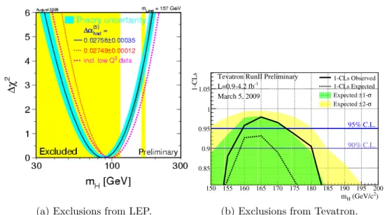
Until now the Higgs boson has not been discovered yet. This is probably due to the weak coupling and its high mass. Its discovery is one of the main goals of the new accelerator LHC. From experiments with LEP the mass of the Higgs boson is excluded below 114.4 GeV [25]. Recently the CDF and D0 experiments at Tevatron could exclude the region 160-170 GeV (see fig. 1.3) [26].

1.2.4 Quantum Chromo Dynamics (QCD)

The QCD introduces a new quantum number named color. It has three possible values: red, green and blue, respectively anti-red, anti-green and anti-blue for anti-quarks. These always combine to a colorless (or “white”) particle. In case of the baryon it means that each of the constituents has a different color (rgb

= white). In case of mesons the quark and the anti quark carry the same, but opposite color (e.g. red and anti-red).

(a) Exclusions from LEP.

2) (GeV/c mH

150 155 160 165 170 175 180 185 190 195 200

1-CLs

0.85 0.9 0.95 1 1.05

L=0.9-4.2 fb-1

March 5, 2009

Tevatron RunII Preliminary 1-CLs Observed 1-CLs Expected 1-σ Expected ±

2-σ Expected ±

95% C.L.

90% C.L.

(b) Exclusions from Tevatron.

Figure 1.3: Exclusion of the Higgs mass m_H made with measurements done at LEP and Tevatron. [27] [26]

The strong force only couples to colored particles. Consequently color is the charge of the QCD. As leptons are colorless and have no known substructure that could carry color, quarks are the only particles that can interact using the strong force.

The underlying symmetry in QCD is SU(3). It postulates eight gauge bosons with spin 1 as mediators. The difference between the eight gluons is the color they are carrying. Each gluon carries the charge of QCD in form of a color and an anticolor.

Hence in an strong interaction color is exchanged between the participants. These can be quarks, but as each gluon carries color, gluons can interact with each other.

They can even form so called “glue balls”.

The strength of the coupling between the colored particle and the gluon is de- scribed by the coupling constantα_s. This “constant” like also the electromagnetic and weak coupling, turn out to be dependant on the energy transfer between the fermions and gauge bosons. For increasing energy transfers the coupling con- stant decreases, going to zero at asymptotic energy transfer. This running of the coupling constant is called asymptotic freedom.

As already stated above, quarks have never been observed as free particles. If one would try to take a meson and “pull” at the two quarks the amount of energy needed increases with the quark separation. Once enough energy is acquired (E >

2m_hadron) it is used to create a new quark - anti-quark pair. These just created quarks will bind to the two original quarks and form two new Mesons where the quarks again are not separated by much (less than about 1 fermi). This property of QCD is called confinement.

1.3 Beyond the Standard Model

Although the Standard Model and its predictions are a great success it cannot be the final theory. It does not explain the asymmetry between matter and antimat- ter sufficiently as well it totally lacks a description of dark matter. Hence there are a lot of theories going beyond the current Standard Model, like the Grand Unified Theories.

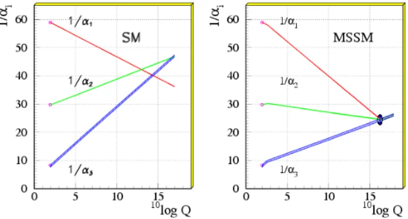
The Standard Model includes the unification of the electromagnetic and the weak force at energies of around 100 GeV. The SM does not relate the various couplings (electromagnetic, weak and strong). A theory which describes the unification of all three forces is called aGrand Unified Theory (GUT). The unification is expected to happen around 10¹⁵GeV at the so called GUT-scale.

1.3.1 Super Symmetry (SUSY)

The Super-Symmetry (SUSY) theory is a potential GUT candidate and also an attractive theory to provide candidate particles for the dark matter. Within this symmetry each elementary fermion is associated with a corresponding boson called Superpartner. Also for the gauge bosons superpartners with spin¹/2 exists.

All these superpartners must be in a mass range unreached by previous particle accelerators.

Figure 1.4: Unification of the coupling constants at the GUT scale in the MSSM.

[25, fig. 15.1]

The Minimal Supersymmetric Standard Model (MSSM) is a minimal extension to the Standard Model including Super Symmetry which could provide the unifi- cation (see fig. 1.4). It adds another Higgs-doublet for the spontaneous symmetry breaking of the electroweak theory resulting in a total of 5 Higgs particles:h⁰ (CP even boson, similar energy as SM Higgs boson), H⁰ (CP even boson), A⁰ (CP

odd boson),H (charged fermions). Some of the Superpartners postulated in the MSSM are in the energy range of the Large Hadron Collider [1] at CERN [2], which will hopefully be found at the LHC at an energy scale of order TeV.

If Supersymmetry will be found around the Terascale (∼ 1 TeV), there is a pre- diction that the three coupling constants will unite.

1.3.2 Other extensions

Apart from Super Symmetry there are other theories extending the Standard Model [28] [29]. But they all share the prediction of additional particles at the Terascale. Hence new accelerators and detectors like the LHC and the ILC are needed for verification.

In this chapter we will present the International Linear Collider and discuss the physical principles of a particle detector on the example of one of the ILC detec- tor concepts. Last but not least the CALICE collaboration and their prototype detectors are presented.

2.1 The International Linear Collider

2.1.1 Motivation for a new e⁺e⁻ - collider

The Large Hadron Collider (LHC) [1] is a proton storage ring reaching energies up to 14 TeV. Therefore the two general purpose detectors ATLAS and CMS are capable of finding the Higgs Boson as well as new physics such as super symmetric particles.

But using a proton collider for this studies of the Terascale has some limitations.

Unlike leptons protons have a substructure made of partons. The protons energy is not split equally among the partons, and it is not measurable which parton has how much energy prior to the collision. The actual collision happens with these partons, not the the proton. Consequently the energy of the collision partners is unknown. And unlike leptons partons can interact via the strong force resulting in a pile up of underlying events which is especially large at this high luminosity and cross section. Consequently it has larger systematic errors.

Therefore there is a high discovery potential for new physics at the LHC, but precision measurements and detailed studies of the new physics spectrum have to be done with a lepton collider. Currently the only leptons which can be handled without problems for such a purpose are electrons e⁻ and positrons e⁺.

2.1.2 Reasons for a new linear collider

Using a circular accelerator like the LHC storage ring has nice benefits. As the particles are passing the accelerating RF structure several times, one does not need many of these expensive devices when increasing the energy. Additionally the

13

particles that didn’t collide can be reused at the next interaction point while still having the same energy. This saves effort necessary for creating and accelerating new particles. The downside of circular accelerators is that synchrotron radiation appears.

Synchrotron radiation is radiation emitted from an accelerated charged particle.

As a particle moving on a circle with radius R is continuously accelerated to the center of the ring, the energy loss due to radiation is [30, p. 226]:

P = dE

dt ≈ 2cq² 3

γ⁴

R² = 2cq² 3

E⁴

m⁴c⁸R² (2.1)

As one can see the mass mof the colliding particle contributes with a power of 4.

Compared to the proton the electron is ≈2000 times lighter, resulting in a much larger synchrotron radiation at the same energy:

P_e P_p =

2cq² 3

E⁴ m⁴_ec⁸R²_e 2cq²

3 E⁴ m⁴_pc⁸R²_p

= (m_p)⁴R²_p (₂₀₀₀^mp )⁴R²_e

= 1.6·10¹³· R²_p R²_e

(2.2)

This lost energy has to be put back in and is a major cost driver for maintaining the beam. Therefore another increase is not an option. As the energy E of the particle is fixed from our analysis the only parameter that is changeable is the radius R. But the radius contributes only with a power of 2.

The predecessor of LHC was the e⁺e⁻ - storage ring LEP built in the same tunnel (circumference: 27 km) with a maximum energy of ≈ 209 GeV [31]. An e⁺e⁻ - storage ring reaching an energy of 1 TeV without increasing synchrotron radiation has therefore to have a ≈27 times larger radius than LEP/LHC. Such a machine is not feasible to built.

Synchrotron radiation is only a feature of circular acceleration. Hence using a linear accelerator circumvents this problem.

2.1.3 The ILC

The International Linear Collider (ILC, see fig. 2.1) is a planned future 31 km long linear e⁺e⁻ collider. It is the unification of several international projects from different parts of the world: the Americas, Europe and Asia. The Reference Design Report (RDR) [32] was published in August 2007.

The ILC is designed to be complementary to LHC. It’s purpose is the precise measurement of new physics as well as tests of the Standard Model (SM) at energies of up to 500 GeV, later on upgradeable to 1000 GeV. It is designed for high luminosity with the ability to collide polarized beams.

Main Linac

Damping Rings

Main Linac 31 km

e⁺ e⁻

e⁻

Positrons

Electrons

Undulator

Detectors Electron

Source

Beam Delivery System

Figure 2.1: The layout of the ILC.

2.1.4 Detector concepts

Unlike the LHC the ILC will only have a single interaction point. In order to provide a systematic cross check it is discussed to use two detectors in a so called

“push-pull” setup, changing every now and then the currently active detector.

There are currently three different detector concepts, each with their own Letter of Intent (LoI). The International Detector Advisory Group [33] will decide which of the following concepts will be approved:

ILD “International Large Detector” [3]

SiD “Silicon Detector” [34]

4th the so called “4th detector concept” [35]

As this thesis shows results created with the results of the prototype of a hadronic calorimeter under discussion for ILD, we will only discuss this detector concept.

2.1.5 ILC Detector requirements

The goal of the ILC is the precise measurement of new physics at high energy scales (up to 1 TeV) as well as studying Standard Model physics with high pre- cision. This includes top physics, physics with Z/W Bosons and heavy flavour physics as well potential particles like Higgs or SUSY particles. All of these anal- ysis require that multi-jet final states can be measured and reconstructed very precisely.

One of these requirements is the possibility to distinguish jets from hadronic W and Z decays, enforcing a jet energy resolution of σ_E/E ≈3−4% or 30%/√

E. Also with such a good resolution it is possible to account for invisible energy in events like neutrinos or possibly light super symmetric particles. To achieve this the ILD and the SiD detector concepts use so called Particle Flow Algorithms (PFA, see section 2.2.4).

2.2 The International Large Detector (ILD)

The International Large Detector (ILD) is one of the ILC detector concepts. Al- though the Letter of Intent [3] was already presented to the International Detector Advisory Group (IDAG) [33] in the end of march 2009, the design parameters are not totally fixed yet as there is a lot of ongoing research, so any numbers presented here may change in the future.

2.2.1 Passage of charged particles through matter

The principle of every detector is the energy loss of particles when passing through matter. When charged particles pass through matter they undergo a lot of inter- actions resulting in energy loss and deflection from the original flight direction.

These reasons for this are:

• inelastic collisions with the materials atomic electrons

• elastic scattering with the nuclei

• emission of Cherenkov-Radiation

• nuclear reactions

• bremsstrahlung

Inelastic collisions: Bethe Bloch

For heavy particles the main energy loss is due to inelastic collisions with the atomic electrons where heavy means anything with a mass greater than the elec- trons mass m > m_e. Bethe and Bloch [36] derived a formula based on quantum mechanical considerations describing the mean energy loss per unit path ^dE_dx. Ex- perience shows that this formula is a good approximation for a wide range of materials if the densityρ is taken into account. Therefore it is usually written as:

−1 ρ

dE

dx = constZ A

z²

β² ln2m_ec²β²γ²

I −β²− δ 2

!

(2.3)

const ≈0.307

A mass number of material Z atomic number of material

z charge of incoming particle m_e electron mass

β = ^v_c γ = √¹

1−β²

δ density correction factor I mean excitation potential

This formula is not valid for electrons as for a collision of partners with equal mass we cannot assume that the path is undeflected. Moreover the collision of electron- electron introduces a maximum energy transfer per collision of 2 times the kinetic energyE_kinof the incident electron. However, there is a similar, corrected formula.

For more details see section 2.2 and 2.4 in [37].

As seen in fig. 2.2 the mean energy loss per unit path length is strongly energy dependant with a minimum at around βγ ≈3−4. Particles at that speed loose a minimum of energy and a therefore called:

Minimum Ionizing Particle (MIP)

A MIP is a particle that has such a speed that the mean energy loss is minimal when passing through matter.

As seen in fig. 2.2 the energy loss rises only slowly with increased energy. Thus particles with βγ >3 are often called MIP as well.

If the energy deposited by 1 MIP in an arbitrary detector is known, one can use a MIP as an energy unit.

Radiation losses: Bremsstrahlung and Cherenkov radiation

As seen in fig. 2.2 further losses due to radiation have to be considered forβγ &

1000. For electrons this is already the case for an energy of 10 MeV or higher.

There are two main effects: Bremsstrahlung and Cherenkov radiation.

Bremsstrahlung is a radiation coming from deflection of the incident particle at the electric field of the materials hull electrons. This deflection is an acceleration into a new direction and any acceleration introduces radiation. The energy for this radiation is taken from the particle.

The second effect is Cherenkov radiation. This arises when a particle moves with a speedv faster than the speed of lightc_m =^c/nin a medium with refractive index n. Due to polarization effects a light cone at well defined angle θ_C is emitted.

The angle is dependant on the refractive index n and the speed of the particle v =cβ [37]:

cosθC = 1

βn (2.4)

This can be used in detectors for speed classification and therefore - if the energy is known - for particle identification.

Muon momentum 1

10 100

Stopping power [MeV cm2/g] Lindhard- Scharff

Bethe-Bloch Radiative

Radiative effects reach 1%

µ⁺ on Cu

Without δ Radiative

losses

0.001 0.01 0.1 1 10 βγ 100 1000 10⁴ 10⁵ 10⁶

[MeV/c] [GeV/c]

100 10

1

0.1 1 10 100 1 10 100

[TeV/c] Anderson-

Ziegler

Nuclear losses

Minimum ionization

E_µc

µ⁻

Figure 2.2: Energy loss for muons when passing through matter [25, fig. 27.1].

Energy loss in thin absorbers

Note that the Bethe-Bloch formula describes only the mean energy loss. Two particles of the same energy flying through the same material of the same strength don’t have to undergo the same number and type of collisions and hence the particle energy after the passage can vary. If the material is thick enough the distribution of the particle energy after the passage is Gaussian. This follows from the central limit theorem, which states that each distribution converges to a Gaussian if the number of repetitions, in this case collisions, becomes very large.

If on the other hand the material is very thin the central limit theorem is not applicable and the distribution of the energy loss becomes very complicated.

Large energy transfers from single interactions can occur as well as “one-shot”

energy loss due to bremsstrahlung, δ-electrons and other effects. These are rare

energy deposition [MIP]

propability

Figure 2.3: The Landau distribution describing mean energy loss for particles passing through thin matter.

and would be negligible for a large number of collisions but for thin layers it adds a large tail to the distribution. Landau described the energy loss in [38]. The resulting distribution is named after him and can be seen in fig. 2.3.

The peak of the Landau distribution is called the Most Probable Value (MPV).

2.2.2 Tracking Detector

A tracking detector searches for tracks of charged particles. It makes use of the ionization of matter through energy deposition as described in the last chapter.

If a magnetic field B is applied, the particle’s path will be curved due to the Lorentz forceFL and the radial forceFr. The radius r of the curve is dependant on the particles momentump, its charge qand the intensity of the magnetic field B.

FL=Fr ⇒ p

r =qB (2.5)

Most charged particles created in a collision experiment like the ILC posess a positve or negative elementary charge. Thus for a given magnetic field B the detection of the track and its radiusryields in the particles transverse momentum p_t.

Its resolution is defined by [39]:

σ(p_t)

p_t ∝ σ(x) B

s 720

N + 4p_t (2.6)

WhereN is the number andσ(x) is the spatial resolution of the measured points.

Note that the resolution ^σ(p_pt^t) increases for higher p_t.

Any interaction of the particle will change its energy and direction of flight through multiple scattering. Deviations from the original flight path increase the momentum resolution. Thus in detectors the number of collisions is reduced by either using very thin detectors (typically silicon based), or detectors with a very low density (e.g. gas).

For covering a large area of the particle’s flight path a tracking chamber filled with gas can provid many measuring points N. In case of the ILD a Time Projection Chamber [3] [37] is used.

Silicon based detectors, often called vertex detectors, provide only few measuring pointsN, but have an excellent spatial resolution and are usually placed near the interaction point.

2.2.3 Electromagnetic and Hadronic Calorimeters

Interaction of Photons with matter

A photon γ passing through matter can undergo several interaction types:

Photoelectric effect

The photon gets absorbed by an atomic hull electron which uses the energy to leave its bound state. This effect decreases with larger energies and is therefore only dominant at low energies.

Compton scattering

In this case the incident photon scatters on one of the quasi free hull elec- trons and deposits energy in dependence of its angle of reflection. Just as the photo electric effect it decreases with larger energy but is still the dom- inating factor in the middle energy range before pair production starts.

Pair production

As soon as the energy of the incident photon is large enough to produce an e⁺e⁻ - pair, i.e. its energy E is larger than twice the mass of the electron m_e (E ≥2m_e), it becomes the dominant interaction effect.

Electromagnetic Showers

An Electromagnetic (EM) shower is a series of pair production and bremsstrahlung effects forming a cascade. A photon will undergo pair produc- tion and both the electron and the positron will create additional photons via bremsstrahlung. These will create other e⁺e⁻ pairs which will produce more γ etc. until the energy of the incident particle is splitted so often that the single daughter particles don’t possess enough energy for creating further particles. In a rough estimation the number of particles N produced is proportional to the energy E of the incident particle:

N ∝E (2.7)

The evolution of an EM shower is described by the radiation lengthX₀. radiation length X₀

X₀ is both the⁷/⁹th of the mean free path of an high energy photon before it undergoes pair production as well as the path where an electron looses all but ¹/^e of it’s energy due to bremsstrahlung.

Hadronic Showers

Hadronic interaction is based on the strong force. This has very limited range and it can, unlike EM interaction which can interact with the hull electrons, only interact with the atomic nuclei. Consequently hadronic interactions are not happening as often as EM interactions and the typical shower length is bigger in the hadronic case. But once a particle collides with a nucleus it can undergo a lot of different reactions. This includes the creation of EM particles (usually when a π⁰ decays to 2γ) which create secondary EM cascades within the hadron shower.

The length of the hadronic shower is measured in the interaction length λ. nuclear interaction length

The nuclear interaction lengthλof an absorber medium is defined as the av- erage distance a high-energy hadron has to travel inside that medium before a nuclear interaction occurs [40]. The probability that such an interaction does not occur after a traveled distance of z is:

P =e^−λz (2.8)

λ is inversely proportional to the total cross section, hence it is particle dependant:

σ_tot ∝ 1

λ (2.9)

Depending on the material, λ is usually much bigger than X₀. Therefore any EM particles will be stopped earlier and the size of EM subshowers in hadronic cascades is small as well.

Calorimeters

In general each particle detector tries to make use of the energy the passing particle deposits for measurements. These can be separated into two classes: On the one hand there are tracking detectors that want to keep the energy loss as low as possible, so that the particle won’t get disturbed too much.

Calorimeters on the other hand are detectors that want to measure the total energy of the incoming particle by completely stopping it within its material.

They thereby make use of the developments of EM and hadronic showers.

Depending on the material the interaction length is usually much bigger than the radiation length (λX₀). Thus there are calorimeters specialized in measuring just EM or just hadronic (with EM subshowers) showers. They are called electro- magnetic and hadronic calorimeters respectively. EM calorimeters usually have a length of several 10 X0 (and 1λ) while hadronic calorimeters have a typical length of 5−10λ. The probability that a hadronic particle can pass a 5λ calorimeter without interacting is according to equation 2.8:

P(5·λ) = e^−5λλ ≈0,67% (2.10) There are two types of calorimeters:

Homogeneous calorimeters

It consists entirely out of active material, i.e. a particle passing anywhere through the calorimeter will be measurable.

Sampling calorimeters

In order to reduce space usage, which effectively minimizes material and therefore costs, a sampling calorimeter consists out of active layers which are capable of measuring particles, and passive material called absorber.

For absorbers usually very dense matter like lead or steel is used. Typically many layers of both types are placed back to back, creating a sandwich like structure.

The signal measured in the calorimeter underlies some fluctuations dependant on the energy of the incident particle. To get the relative fluctuations, one measures the width of the measured energy σ_E over the energy E, which is influence by:

a stochastic fluctuations. In principle the calorimeter counts the number of secondary particles of a shower to measure the initial particle’s energy.