Decision Trees in the Semi-Digital Hadronic Calorimeter Prototype

(1)

Preprint typeset in JINST style - HYPER VERSION

Particle Identification Using Boosted

Decision Trees in the Semi-Digital Hadronic Calorimeter Prototype

The CALICE Collaboration

D. Boumediene,

Université Clermont Auvergne, Université Blaise Pascal, CNRS/IN2P3, LPC, 4 Av. Blaise Pascal, TSA/CS 60026, F-63178 Aubière, France

A. Pingault, M. Tytgat

Ghent University, Department of Physics and Astronomy, Proeftuinstraat 86, B-9000 Gent, Belgium

B. Bilki, D. Northacker, Y. Onel

University of Iowa, Dept. of Physics and Astronomy, 203 Van Allen Hall, Iowa City, IA 52242-1479, USA

G. Cho, D-W. Kim, S. C. Lee, W. Park, S. Vallecorsa Gangneung-Wonju National University Gangneung 25457, South Korea

Y. Deguchi, K. Kawagoe, Y. Miura, R. Mori, I. Sekiya, T. Suehara, T. Yoshioka Department of Physics and Research Center for Advanced Particle Physics, Kyushu

University, 744 Motooka, Nishi-ku, Fukuoka 819-0395, Japan

L. Caponetto, C. Combaret, R. Ete ^∗ , G. Garillot, G. Grenier, J-C. Ianigro, T.

Kurca, I. Laktineh, B. Liu ^a , B. Li, N. Lumb, H. Mathez, L. Mirabito, A. Steen ^† Univ Lyon, Univ CLaude Bernard Lyon 1, CNRS/IN2P3, IP2I Lyon, F-69622

Villeurbanne, France

E. Calvo Alamillo, M.C. Fouz, J. Marin, J. Navarrete, J. Puerta Pelayo, A. Verdugo

CIEMAT, Centro de Investigaciones Energeticas, Medioambientales y Tecnologicas, Madrid, Spain

F. Corriveau, B. Freund ^‡

Department of Physics, McGill University, Ernest Rutherford Physics Bldg., 3600 University Ave., Montréal, Québec, Canada H3A 2T8

arXiv:2004.02972v1 [physics.ins-det] 6 Apr 2020

(2)

M. Chadeeva, M. Danilov ^§

P. N. Lebedev Physical Institute of the Russian Academy of Sciences, 53 Leninsky prospekt, Moscow, 119991 Russia

L. Emberger, C. Graf, F. Simon, C. Winter

Max-Planck-Institut für Physik, Föhringer Ring 6, D-80805 Munich, Germany J. Bonis, D. Breton, P. Cornebise, A. Gallas, J. Jeglot, A. Irles, J. Maalmi,

R. Pöschl, A. Thiebault, F. Richard, D. Zerwas

Universit ˝ O Paris-Saclay, CNRS/IN2P3, IJCLab, 91405 Orsay, France M. Anduze, V. Balagura, V. Boudry, J-C. Brient, E. Edy, F. Gastaldi,

R. Guillaumat, F. Magniette, J. Nanni, H. Videau

Laboratoire Leprince-Ringuet (LLR) – CNRS, École polytechnique, Institut Polytechnique de Paris Palaiseau, F-91128 France

S. Callier, F. Dulucq, Ch. de la Taille, G. Martin-Chassard, L. Raux, N. Seguin-Moreau

Laboratoire OMEGA – École Polytechnique-CNRS/IN2P3, Palaiseau, F-91128 France J. Cvach, M. Janata, M. Kovalcuk, J. Kvasnicka, I. Polak, J. Smolik, V. Vrba,

J. Zalesak, J. Zuklin

Institute of Physics, The Czech Academy of Sciences, Na Slovance 2, CZ-18221 Prague 8, Czech Republic

Y.Y. Duan, S. Li, J. Guo, J.F. Hu, F. Lagarde, B. Liu ^a , Q.P. Shen, X. Wang, W.H. Wu, H.J. Yang, Y.F. Zhu

Tsung-Dao Lee Institute, Institute of Nuclear and Particle Physics, School of Physics and Astronomy, Shanghai Jiao Tong University, Key Laboratory for Particle Physics, Astrophysics and Cosmology (Ministry of Education), Shanghai Key Laboratory for Particle Physics and Cosmology, 800 Dongchuan Road, Shanghai, 200240, P. R. China

a Corresponding author

E-mail: b.Liu@ipnl.in2p3.fr, 610412075@sjtu.edu.cn

A BSTRACT : The CALICE Semi-Digital Hadronic CALorimeter (SDHCAL) prototype us-

ing Glass Resistive Plate Chambers as a sensitive medium is the first technological proto-

type of a family of high-granularity calorimeters developed by the CALICE collaboration

to equip the experiments of future leptonic colliders. It was exposed to beams of hadrons,

electrons and muons several times in the CERN PS and SPS beamlines between 2012 and

2018. We present here a new method of particle identification within the SDHCAL us-

ing the Boosted Decision Trees (BDT) method applied to the data collected in 2015. The

performance of the method is tested first with Geant4-based simulated events and then

on the data collected by the SDHCAL in the energy range between 10 and 80 GeV with

10 GeV energy steps. The BDT method is then used to reject the electrons and muons that

contaminate the SPS hadron beams.

(3)

K EYWORDS : Calorimeters, MVA.

∗

Now at DESY

†

Now at NTU

‡

Also at Argonne National Laboratory

§

Also at MIPT

(4)

1. Introduction 1

2. Monte Carlo samples and beam data samples 2

3. Particle identification using Boosted Decision Trees 3

3.1 BDT input variables 3

3.2 The two approaches to build the BDT-based classifier 5

3.2.1 MC Training Approach 5

3.2.2 Data Training Approach 10

4. Results 11

5. Conclusion 13

6. Acknowledgements 14

1. Introduction

1

The Semi-Digital Hadronic CALorimeter (SDHCAL) [1] is the first of a series of techno-

2

logical high-granularity prototypes developed by the CALICE collaboration. These tech-

3

nological prototypes have their readout electronics embedded in the detector and they are

4

power-pulsed to reduce the power consumption in experiments proposed within the Inter-

5

national Linear Collider (ILC) project [2]. The mechanical structure of these prototypes is

6

part of their absorber. All these aspects increase the compactness of the calorimeters and

7

improve their suitability to apply the Particle Flow Algorithm (PFA) techniques [3, 4, 5].

8

The SDHCAL is made of 48 active layers, each of them equipped with a 1 m × 1 m Glass

9

Resistive Plate Chamber (GRPC) and an Active Sensor Unit (ASU) of the same size host-

10

ing on one face (the one in contact with the GRPC) pickup pads of 1 cm × 1 cm and 144

11

HARDROC2 ASICs [6] on the the other face. The GRPC and the ASU are assembled

12

within a cassette made of two stainless steel plates, 2.5 mm thick each. The 48 cassettes

13

are inserted in a self-supporting mechanical structure made of 51 plates, 15 mm thick each,

14

of the same material as the cassettes, bringing the total absorber thickness to 20 mm per

15

layer. The empty space between two consecutive plates is 13 mm to allow the insertion

16

of one cassette of 11 mm thickness. The HARDROC2 ASIC has 64 channels to read out

17

(5)

64 pickup pads. Each channel has three parallel digital circuits whose parameters can be

18

configured to provide 2-bit encoded information indicating if the charge seen by each pad

19

has passed any of the three different thresholds associated to each digital circuit. This

20

multi-threshold readout is proposed to improve on the energy reconstruction of hadronic

21

showers at high energy (> 30 GeV) with respect to the simple binary readout mode as

22

explained in Ref. [7].

23

The SDHCAL was exposed several times to different kinds of particle beams in the

24

CERN PS and SPS beamlines between 2012 and 2018. The energy reconstruction of

25

hadronic showers within the SDHCAL using the associated number of fired pads with

26

multi-threshold readout information is presented in Ref. [7]. The contamination of the

27

SPS hadron beams such as electrons and muons and the absence of Cherenkov counters

28

during the data taking require the use of the event topology to select the hadronic events

29

before reconstructing their energy. Although the rejection of muons based on the average

30

number of hits per crossed layer is efficient, the rejection of electrons is more difficult

31

because some hadronic showers behave in similar way as the electromagnetic ones in

32

particular at low energy. To reject the electron events, the analysis presented in Ref. [7]

33

requires the shower to start after the fifth layer. Almost all of the electrons are expected to

34

start showering before crossing the equivalent of 6 radiation lengths (X ₀ ) ¹ . Although this

35

selection is found to have no impact on the hadronic energy reconstruction, it represents

36

0.6 interaction length (λ _I ) and thus reduces the amount of the hadronic showers available

37

for analysis.

38

In this paper we explore another method to reject the electron and muon contamina-

39

tions, that is not based on the shower start requirement and does thus preserve the statistics.

40

The new method is based on Boosted Decision Trees (BDT) [8, 9], a part of so-called Mu-

41

tiVariate Analysis (TMVA) technique [10]. In the BDT, different variables associated to

42

the topology of the event are exploited in order to distinguish between the hadronic and

43

the electromagnetic showers, and also to identify muons including radiative ones that may

44

exhibit a shower-like shape. In this paper, section 2 introduces the simulation and beam

45

data samples which are used to study the performance of both the BDT and the standard

46

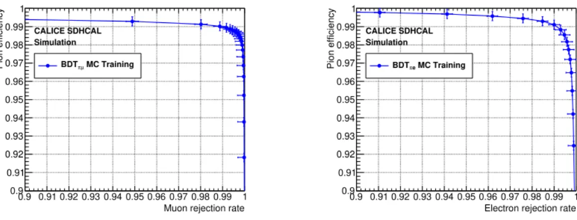
method described in Ref. [7]. Section 3 describes the selected input variables of BDT and

47

the two approaches to build the classifier of BDT. Section 4 presents the results of the

48

hadron selection using BDT. Finally, section 5 gives the conclusion.

49

2. Monte Carlo samples and beam data samples

50

The SDHCAL prototype was exposed to pions, muons and electrons in the SPS of CERN

51

in October 2015. In order to avoid GRPC saturation problems at high particle rate, only

52

runs with a particle rate smaller than 1000 particles/spill are selected for the analysis. In

53

these conditions, pion events at several energy points (10, 20, 30, 40, 50, 60, 70, 80 GeV)

54

1

The longitudinal depth of the SDHCAL prototype layer is about 1.2 X

0

.

(6)

and muon events of 110 GeV were collected as well as electron events of 10, 15, 20,

55

25, 30, 40, 50 GeV. While the electron and muon beams are rather pure, the pion beams

56

are contaminated by two sources. One is the electron contamination despite the use of

57

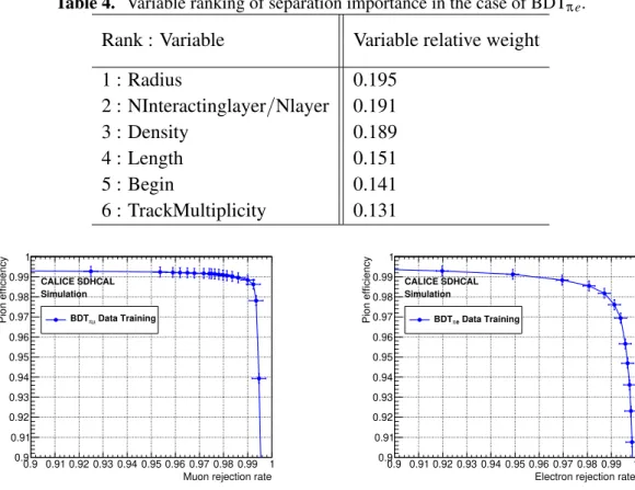
a lead filter to reduce the number of electrons. The other is the muon contamination

58

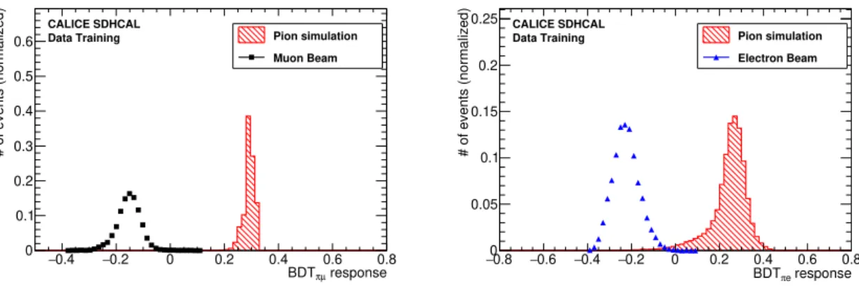
resulting from pions decaying before reaching the prototype. To apply the BDT method,

59

six variables are selected and used in the Toolkit for MultiVariate data Analysis (TMVA)

60

package [10] to build the decision tree.

61

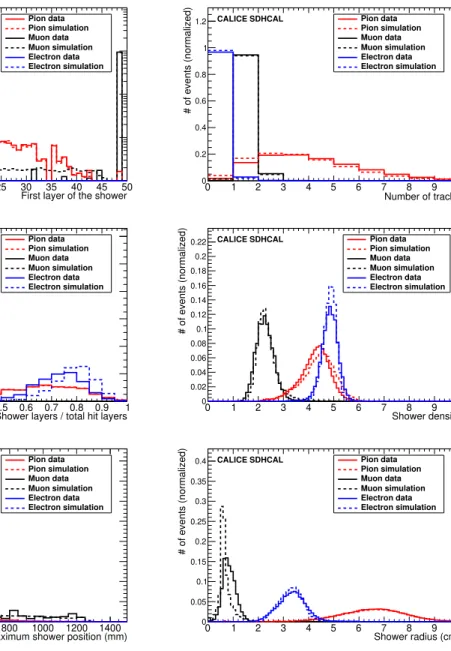
To study the performance of the BDT method, we use the Geant4.9.6 Toolkit pack-

62

age [11] associated to the FTF-BIC ² [12, 13] physics list to generate pion, electron and

63

muon events under the same conditions as in the beam test at CERN-SPS beamline. For

64

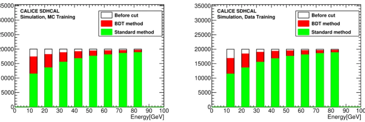
the training of the BDT, 10k events for each energy point from 10 GeV to 80 GeV with a

65

step of 10 GeV for pions, muons and electrons were produced. The same amount of events

66

of each species is produced and used to test the BDT method at the same time. Finally, the

67

pure (> 99.5%) electron and muon data samples ³ are used as validation sets.

68

In order to render the particle identification independent of the energy of the different

69

species and thus to extend the method applied here to a larger scope than the beam purifi-

70

cation, the pion samples of different energies are mixed before using the BDT technique.

71

The same procedure is applied for muon and electron samples.

72

3. Particle identification using Boosted Decision Trees

73

Thanks to the high granularity of the SDHCAL, we can use the MVA methods to mine

74

the information of the shape of electromagnetic and hadronic shower to classify muons,

75

electrons and pions. The BDT method is one of the widely used MVA methods to perform

76

such classification tasks. The BDT is a model that combines many less selective decision

77

trees ⁴ into a strong classifier to achieve a much better performance.

78

3.1 BDT input variables

79

The six variables we use to distinguish hadronic showers from electromagnetic show-

80

ers and from muons are described below. A common right-handed coordinate system is

81

used throughout the SDHCAL whose 48 layers were placed perpendicular to the incoming

82

beams. The origin of the system is defined as the center of the first of the 48 SDHCAL’s

83

layers. The x-y plane is parallel to the SDHCAL layers and referred to as the transverse

84

plane while the z-axis runs parallel to the incoming beam.

85

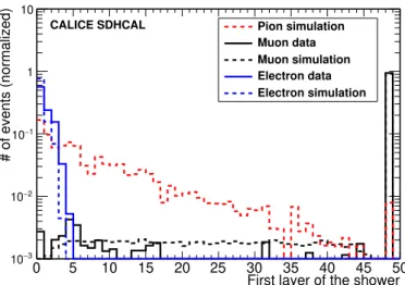
• First layer of the shower (Begin) : The probability of a particle to interact in the

86

calorimeter depends on the particle nature and the calorimeter material properties.

87

2

The FTF model is based on the Fritiof description of string excitation and fragmentation. The BIC model uses Geant4 binary cascade for primary protons and neutrons with energies below 10 GeV. It describes the production of secondary particles produced in interactions of protons and neutrons with nuclei.

3

The purity of these samples is provided by the SPS electron and muon beams.

4

A decision tree takes a set of input variables and splits input data recursively based on those variables.

(7)

The distribution of the coordinate z of the layer in which the first inelastic interaction

88

takes place, follows an exponential law. It is proportional to exp (− _X ^z

0

) for electrons

89

and to exp(− ^z

λ

I

) for pions, where X ₀ and λ _I are effective radiation length and nuclear

90

interaction length for the SDHCAL material composition, respectively. To define the

91

first layer in which the shower starts we look for the first layer along the incoming

92

particle direction, which contains at least 4 fired pads. To eliminate fake shower

93

starts due to accidental noise or a locally high multiplicity, the following 3 layers

94

after the first one are also required to have more than 4 fired pads in each of them.

95

Particles crossing the calorimeter without interaction are assigned the value of 48,

96

which is the case for most of the muons in the studied beam except the radiative

97

ones. Figure 1 shows the distribution of the first layer of the shower in the SDHCAL

98

prototype for pions, electrons and muons as obtained from the simulation and data.

99

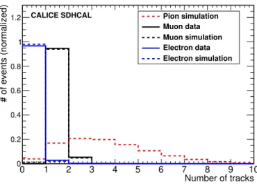
• Number of tracks segments in the shower (TrackMultiplicity): Applying the

100

Hough Transform (HT) technique to single out the tracks in each event as described

101

in Ref. [14], we estimate the number of tracks segments in the pion, electron and

102

muon events. A HT-based segment candidate is considered as a track segment if

103

there are more than 6 aligned hits with not more than one layer separating two con-

104

secutive hits. Electron showers feature almost no track segment while most of the

105

hadronic showers have at least one. For muons, except for some radiative muons,

106

only one track is expected as can be seen in Fig. 2.

107

• Ratio of shower layers over total hit layers (NinteractingLayers/NLayers): This

108

is the ratio between the number of layers in which the Root Mean Square (RMS) of

109

the hits’ position in the x-y plane exceeds 5 cm in both x and y directions and the

110

total number of layers with at least one fired pad. It allows, as can be seen in Fig. 3,

111

an easy discrimination of muons (even the radiative ones) from pions and electrons.

112

It allows also a slight separation between pions and electrons.

113

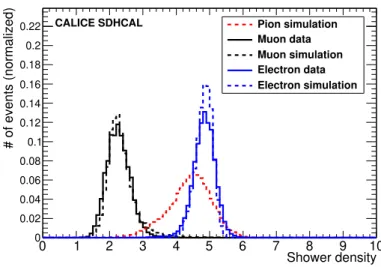
• Shower density (Density): This is the average number of the neighbouring hits

114

located in the 3 × 3 pads around one of the hits including the hit itself in the given

115

event. Figure 4 shows clearly that electromagnetic showers are more compact than

116

the hadronic showers as expected.

117

• Shower radius (Radius): This is the RMS of hits distance with respect to the event

118

axis. To estimate the event axis, the average positions of the hits in each of the ten

119

first fired layers of an event are used to fit a straight line. The straight line is then

120

used as the event axis. Figure 5 shows the average radius of the three particle species

121

in the SDHCAL.

122

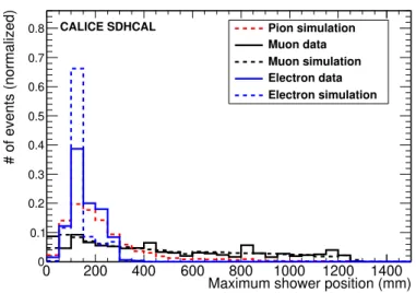
• Shower maximum position (Length): This is the distance between the shower start

123

and the layer where the maximum RMS of hit transverse coordimates with respect

124

(8)

First layer of the shower

0 5 10 15 20 25 30 35 40 45 50

# of events (normalized)

−3

10

−2

10

−1

10 1 10

Pion simulation Muon data Muon simulation Electron data Electron simulation CALICE SDHCAL

Figure 1. Distribution of the first layer of the shower (Begin). Layer 0 refers to the first layer of the prototype. Continuous lines refer to data while dashed ones to the simulation. Layer 48 is the virtual layer after the last layer and used to tag events not fulfilling first layer criteria.

to shower axis is detected. The distribution of this variable for different particle

125

species is shown in Fig. 6.

126

Before using the variables listed above as input to the BDT method, we check that

127

the variables distributions in the simulation are in agreement with data for the muon and

128

electron beams which are quite pure. Figures 1 - 6 show that there is globally a good

129

agreement for the six variables of the two species even though the agreement is not perfect

130

in particular for electrons.

131

3.2 The two approaches to build the BDT-based classifier

132

In order to take into account the small difference observed in some variable distributions

133

between data and simulation, and to cross-check the particle identification using the BDT

134

method, we adopt two different training strategies for the BDT-based classifier. The first

135

approach, referred to as MC Training, uses simulation samples of pions, electrons and

136

muons as training sets. The second, referred to as Data Training, uses simulation samples

137

of pions but electron and muon samples taken from data as training sets.

138

3.2.1 MC Training Approach

139

The six variables of the simulated pion, muon and electron events described in section

140

3.1 are used for the training and testing of the classifier. Events are chosen in alternating

141

turns for the training and test samples as they occur in the source trees until the desired

142

numbers of training and test events are selected. The training and test samples contain

143

the same number of events for each event class. Independent samples of signal events

144

(9)

Number of tracks

0 1 2 3 4 5 6 7 8 9 10

# of events (normalized)

0 0.2 0.4 0.6 0.8 1

1.2 Pion simulation

Muon data Muon simulation Electron data Electron simulation CALICE SDHCAL

Figure 2. Distribution of number of the tracks in the shower (TrackMultiplicity). Continuous lines refer to data while dashed ones to the simulation.

Shower layers / total hit layers 0 0.1 0.2 0.3 0.4 0.5 0.6 0.7 0.8 0.9 1

# of events (normalized)

0 0.2 0.4 0.6 0.8 1

Figure 3. Distribution of ratio of the number of layers in which RMS of the hits’ position in the x-y plane exceeds 5 cm over the total number of fired layers (NinteractingLayers/NLayers).

Continuous lines refer to data while dashed ones to the simulation.

(pions) and of the different background contributions (electron and muons) are used. The

145

ratio between signal and each background (electron or muon) events is 1 for training and

146

test samples. After the training, the BDT provides the relative weight of each variable

147

as a measure of distinguishing signal from background. Two BDT-based classifiers are

148

proposed here. The first (BDT _{π µ} ) is used to discriminate pions against muons and the

149

second (BDT _π _e ) to discriminate against electrons. Table 1 shows the variable ranking

150

according to their separation power in the BDT _{π µ} while Tab. 2 gives their separation power

151

(10)

Shower density

0 1 2 3 4 5 6 7 8 9 10

# of events (normalized)

0 0.02 0.04 0.06 0.08 0.1 0.12 0.14 0.16 0.18 0.2

Figure 4. Distribution of the average number of neighbouring hits surrounding one hit (Density).

Continuous lines refer to data while dashed ones to the simulation.

Shower radius (cm)

0 1 2 3 4 5 6 7 8 9 10

# of events (normalized)

0 0.05 0.1 0.15 0.2 0.25 0.3 0.35

Figure 5. Distribution of the average radius of the shower (Radius). Continuous lines refer to data while dashed ones to the simulation.

in the case of BDT πe . The BDT algorithm using the variables and their respective weights

152

is then applied to the test samples. The output of the BDT applied to each of the test sample

153

events is a variable belonging to the interval [-1,1] with the positive value representing

154

more signal-like events and the negative more background-like events.

155

Figure 7 (left) shows the output of the BDT for a test sample made of pions and

156

muons while Fig. 7 (right) shows the output for a test sample made of pions and elec-

157

trons. The values differ significantly for signal and background suggesting thus a large

158

separation power of the BDT approach. This is confirmed by Fig. 8. The pion selection

159

(11)

Maximum shower position (mm) 0 200 400 600 800 1000 1200 1400

# of events (normalized)

0 0.1 0.2 0.3 0.4 0.5 0.6 0.7

Figure 6. Distribution of the position of the layer with the maximum radius (Length). Continuous lines refer to data while dashed ones to the simulation.

Table 1. Variable ranking of separation power in the case of BDT

π µ

.

Rank : Variable Variable relative weight

1 : Length 0.233

2 : Density 0.225

3 : NInteractinglayer/Nlayer 0.163

4 : Radius 0.160

5 : Begin 0.139

6 : TrackMultiplicity 0.080

Table 2. Variable ranking of separation power in the case of BDT

πe

.

Rank : Variable Variable relative weight

1 : Radius 0.204

2 : NInteractinglayer/Nlayer 0.203

3 : Density 0.194

4 : Length 0.151

5 : Begin 0.145

6 : TrackMultiplicity 0.101

efficiency versus the muon (electron) rejection of the test sample is shown in Fig. 9 (left)

160

and Fig. 9 (right), respectively. A pion selection efficiency exceeding 99% with a muon

161

and electron rejection of the same level (> 99%) can be achieved.

162

In order to check the validity of these two classifiers, we use the pure beam samples of

163

(12)

response

µ

BDTπ

0.4

− −0.2 0 0.2 0.4 0.6 0.8

# of events (normalized)

0 0.05 0.1 0.15 0.2 0.25 0.3 0.35 0.4 0.45

Pion simulation Muon simulation CALICE SDHCAL

Simulation, MC Training

response

e

BDTπ

0.4

− −0.2 0 0.2 0.4 0.6

0 0.02 0.04 0.06 0.08 0.1 0.12 0.14 0.16 0.18 0.2

Electron simulation CALICE SDHCAL

Figure 7. The BDT output of the BDT

π µ

(left) and BDT

πe

(right) built with simulation samples.

response

µ

BDTπ

−0.4 −0.3 −0.2 −0.1 0 0.1 0.2 0.3 0.4

Pion efficiency

0.3 0.4 0.5 0.6 0.7 0.8 0.9 1 1.1 1.2

Muon rejection rate

0.3 0.4 0.5 0.6 0.7 0.8 0.9 1 1.1 1.2 Pion Muon CALICE SDHCAL

response

e

BDTπ

0.4

− −0.3 −0.2 −0.1 0 0.1 0.2 0.3 0.4

Pion efficiency

0.3 0.4 0.5 0.6 0.7 0.8 0.9 1 1.1 1.2

Electron rejection rate

0.3 0.4 0.5 0.6 0.7 0.8 0.9 1 1.1 1.2 Pion Electron CALICE SDHCAL

Figure 8. Pion efficiency and muon rejection rate (left) and pion efficiency and electron rejection rate (right) as a function of the BDT output.

muons and electrons. Figure 10 (left) shows the BDT output of BDT _{π µ} and Fig. 10 (right)

164

shows the case of BDT _πe . Beam muon results show a good agreement with respect to the

165

simulated events. A slight shift of the beam electron shape is observed with respect to the

166

one obtained from the simulated events. This difference is most probably due to the fact

167

that the distribution of some variables in data and in the simulation are not identical. Next,

168

as a first step of purifying the collected hadronic data events we apply the pion-muon

169

classifier. Figure 10 (left) shows the BDT _{π µ} response applied to the collected hadron

170

events in the SDHCAL. We can clearly see that there are two maxima. One maximum in

171

the muon range corresponds to the muon contamination of pion data and another one in the

172

pion range. Hence, to ensure the rejection of the muons in the sample, the BDT variable is

173

required to be > 0.1. The second step is to apply the BDT _π _e to the remaining of the pion

174

sample. Figure 10 (right) shows the BDT _πe output. In order to eliminate the maximum

175

of the electrons contamination and get almost a pure ( > 99.5%) pion sample with limited

176

loss of pion events, we apply to the pion samples a BDT _πe cut of 0.05.

177

(13)

Muon rejection rate 0.9 0.91 0.92 0.93 0.94 0.95 0.96 0.97 0.98 0.99 1

Pion efficiency

0.9 0.91 0.92 0.93 0.94 0.95 0.96 0.97 0.98 0.99 1

MC Training

µ

BDTπ

CALICE SDHCAL Simulation

Electron rejection rate 0.9 0.91 0.92 0.93 0.94 0.95 0.96 0.97 0.98 0.99 1

Pion efficiency

0.9 0.91 0.92 0.93 0.94 0.95 0.96 0.97 0.98 0.99 1

MC Training

e

BDTπ

Figure 9. Pion efficiency versus muon rejection rate(left) and pion efficiency versus electron re- jection rate (right).

response

µ

BDTπ

0.4

− −0.2 0 0.2 0.4 0.6 0.8 1

0 0.05 0.1 0.15 0.2 0.25 0.3 0.35 0.4

Pion simulation Muon simulation Pion Beam Muon Beam CALICE SDHCAL

MC Training

response

e

BDTπ

0.4

− −0.2 0 0.2 0.4 0.6

0 0.02 0.04 0.06 0.08 0.1 0.12 0.14 0.16 0.18 0.2

Electron simulation Pion Beam Electron Beam CALICE SDHCAL

MC Training

Figure 10. The BDT output after using the BDT

_{π µ}

on the data pion sample (left) and the BDT output after using the BDT

πe

on the same data pion sample after classified by BDT

_{π µ}

(right). A green arrow is shown on both to indicate the BDT cut applied to clean the pion samples.

3.2.2 Data Training Approach

178

We use the same variables of the MC Training approach on the data samples of muons and

179

electrons but still on the simulated pion samples to build two classifiers. Then we apply

180

the same procedure as the MC Training approach. Table 3 and 4 show the corresponding

181

variables ranking for BDT _{π µ} and BDT _π _e according to their power separation importance.

182

The difference of variables weights of these two tables with respect to those obtained with

183

MC training approach is explained by the slight difference of some variables distributions

184

between data and simulation. Figure 11 left (right) gives the results of pion efficiency

185

and muon (electron) rejection rate. This shows that these two classifiers have very good

186

pion efficiency and high background rejection rate. The left (right) plot of Fig. 12 shows

187

the BDT output of the BDT _{π µ} (BDT _πe ). Clearly these two classifiers have very good

188

separation power. We apply these classifiers to the raw pion beam samples. The results

189

(14)

Table 3. Variable ranking of separation importance in the case of BDT

_{π µ}

.

Rank : Variable Variable relative weight

1 : Length 0.300

2 : Radius 0.230

3 : Density 0.227

4 : Begin 0.103

5 : NInteractinglayer/Nlayer 0.080 6 : TrackMultiplicity 0.060

Table 4. Variable ranking of separation importance in the case of BDT

πe

.

Rank : Variable Variable relative weight

1 : Radius 0.195

2 : NInteractinglayer/Nlayer 0.191

3 : Density 0.189

4 : Length 0.151

5 : Begin 0.141

6 : TrackMultiplicity 0.131

Muon rejection rate 0.9 0.91 0.92 0.93 0.94 0.95 0.96 0.97 0.98 0.99 1

Pion efficiency

0.9 0.91 0.92 0.93 0.94 0.95 0.96 0.97 0.98 0.99 1

Data Training

µ

BDTπ

Electron rejection rate 0.9 0.91 0.92 0.93 0.94 0.95 0.96 0.97 0.98 0.99 1

Pion efficiency

0.9 0.91 0.92 0.93 0.94 0.95 0.96 0.97 0.98 0.99 1

Data Training

e

BDTπ

Figure 11. Pion efficiency versus muon rejection rate (left) and pion efficiency versus electron rejection rate (right).

can be seen in Fig. 13. We apply a BDT cut value of 0.2 in the pion-muon separation stage

190

and then a BDT cut value of 0.05 in the pion-electron separation stage.

191

4. Results

192

The distributions of input variables for the data and simulation events of pion, muon and

193

electron are shown in Fig. 14. Only the pion data sample distributions are obtained after

194

(15)

response

µ

BDTπ

0.4

− −0.2 0 0.2 0.4 0.6 0.8

0 0.1 0.2 0.3 0.4 0.5

Muon Beam CALICE SDHCAL

Data Training

response

e

BDTπ

0.8

− −0.6 −0.4 −0.2 0 0.2 0.4 0.6 0.8

0 0.05 0.1 0.15 0.2 0.25

Pion simulation Electron Beam CALICE SDHCAL

Data Training

Figure 12. BDT output of the BDT

π µ

built with pure beam muons and simulated pion samples (left) and of the BDT

πe

built with pure beam electrons and simulated pion samples (right)

response

µ

BDTπ

0.8

− −0.6 −0.4 −0.2 0 0.2 0.4 0.6 0.8

0 0.1 0.2 0.3 0.4 0.5 0.6 0.7 0.8

Pion simulation Pion Beam Muon Beam CALICE SDHCAL

Data Training

response

e

BDTπ

0.4

− −0.2 0 0.2 0.4 0.6 0.8

0 0.02 0.04 0.06 0.08 0.1 0.12 0.14 0.16 0.18 0.2

Pion simulation Pion Beam Electron Beam CALICE SDHCAL

Data Training

Figure 13. The BDT output after using the BDT

_{π µ}

on the data pion sample (left) and the BDT output after using the BDT

πe

on the same pion sample after classified by BDT

π µ

(right). A green arrow is shown on both to indicate the BDT cut applied to clean the pion samples.

applying the data-based BDT classifiers. A good agreement between the data and simu-

195

lation events for pions is observed. It also confirms the power of the BDT method. The

196

rejection of muons and electrons presented in the pion data sample using the BDT allows

197

us to have more statistics and a rather pure pion sample as explained in the previous sec-

198

tion. Figure 15 shows the results of comparison in event selection between the standard

199

method and the BDT-based method using the simulation samples. For both simulation and

200

beam data, the BDT method leads to more statistics comparing to the standard method [7]

201

in particular at low energy as shown in Fig. 16 for the comparison of the selected events

202

as a function of the total number of hits for the 10 GeV pion beam data. We also do not

203

observe any significant deviation of energy resolution when applying the standard energy

204

reconstruction described in Ref. [7] on the pion events selected by the BDT method.

205

(16)

First layer of the shower

0 5 10 15 20 25 30 35 40 45 50

3

10− 2

10−

−1

10 1 10

Pion data Pion simulation Muon data Muon simulation Electron data Electron simulation CALICE SDHCAL

Number of tracks

0 1 2 3 4 5 6 7 8 9 10

0 0.2 0.4 0.6 0.8 1

1.2 Pion data

Shower layers / total hit layers 0 0.1 0.2 0.3 0.4 0.5 0.6 0.7 0.8 0.9 1

0 0.2 0.4 0.6 0.8 1

1.2 Pion data

Shower density

0 1 2 3 4 5 6 7 8 9 10

0 0.02 0.04 0.06 0.08 0.1 0.12 0.14 0.16 0.18 0.2

0.22 Pion data

Maximum shower position (mm) 0 200 400 600 800 1000 1200 1400

0 0.1 0.2 0.3 0.4 0.5 0.6 0.7

0.8 Pion data

Shower radius (cm)

0 1 2 3 4 5 6 7 8 9 10

0 0.05 0.1 0.15 0.2 0.25 0.3 0.35

0.4 Pion data

Figure 14. Distributions of six input variables of electron, muon and pion samples. Continuous lines refer to data and dashed ones to the simulation. The pion samples are classified with the data-based training BDT method and others is obtained without applying BDT-based classifiers.

5. Conclusion

206

A new particle identification method using BDT-based MVA technique is applied to purify

207

the pion events collected at the SPS H2 beamline in 2015 by the CALICE SDHCAL proto-

208

type. The new method uses the topological shape of events associated to muons, electrons

209

and pions in the CALICE SDHCAL to reject the two first species. A significant statis-

210

tical gain is obtained with respect to the standard method used in the work presented in

211

Ref [7]. This statistical gain is particularly significant at energies up to 40 GeV and can be

212

(17)

Energy[GeV]

0 10 20 30 40 50 60 70 80 90 100 0

5000 10000 15000 20000 25000 30000 35000

Before cut BDT method Standard method CALICE SDHCAL

Energy[GeV]

0 10 20 30 40 50 60 70 80 90 100 0

5000 10000 15000 20000 25000 30000 35000

Before cut BDT method Standard method CALICE SDHCAL

Simulation, Data Training

Figure 15. The number of simulated events of different energy points from 10 GeV to 80 GeV before (white) and after applying the standard method (green) or BDT method (red). The left plot shows the results from BDT method with MC Training approach while the right one shows the results with Data Training approach.

Nhit 0 50 100 150 200 250 300 350 400 0

500 1000 1500 2000

2500 BDT method

Standard method CALICE SDHCAL

Pion Beam Energy=10GeV MC Training

Nhit 0 50 100 150 200 250 300 350 400 0

500 1000 1500 2000 2500

BDT method Standard method CALICE SDHCAL

Pion Beam Energy=10GeV Data Training

Figure 16. Distribution of the total number of hits for the 10 GeV pion beam data selected by the standard method (blue) and the BDT method (red). The left plot shows the results from BDT method with MC Training approach while the right one shows the results with Data Training ap- proach.

explained by the fact that the showers that start in the first layers are not all rejected. This

213

gain shows the better efficiency and separation power of the multivariate approach over

214

the cut-based approach of the standard method. The BDT-based particle identification in

215

CALICE SDHCAL is a robust and a reliable method as confirmed by the results of two

216

different training approaches.

217

6. Acknowledgements

218

This study was supported by National Key Programme for S&T Research and Develop-

219

ment (Grant NO. 2016YFA0400400).

220

(18)

References

221

[1] G. Baulieu et al., Construction and commissioning of a technological prototype of a

222

high-granularity semi-digital hadronic calorimeter, JINST 10 (2015) P10039.

223

[2] T. Abe et al., The International Large Detector: Letter of Intent, FERMILAB-LOI-2010-01,

224

FERMILAB-PUB-09-682-E, DESY-2009-87,

225

KEK-REPORT-2009-6, (2010) arXiv:1006.3396.

226

[3] M. A. Thomson, Particle Flow Calorimetry and the PandoraPFA Algorithm, NIMA 611 25

227

(2009), arXiv:0907.3577

228

[4] V. L. Morgunov, Calorimetry design with energy-flow concept (imaging detector for

229

high-energy physics), in Proc of Int. Conf. on Calorimetry (Calor02), (2002) Pasadena, 70

230

[5] J. C. Brient and H. Videau, The calorimetry at the future e+e- linear collider, in Proc. of

231

APS/DPF/DBP summer study on the future of particle physics, (2002) Snowmass, Colorado

232

[hep-ex/0202004]

233

[6] F. Dulucq, C. de la Taille, G. Martin-Chassard, N. Seguin-Moreau, HARDROC: Readout

234

chip for CALICE/EUDET Digital Hadronic Calorimeter, IEEE Nuclear Science Symposuim

235

& Medical Imaging Conference, IEEE, 2010.

236

[7] CALICE collaboration, First results of the CALICE SDHCAL technological prototype,

237

JINST 11 (2016) P04001.

238

[8] B. P. Roe, H. J. Yang, J. Zhu et al., Boosted decision trees as an alternative to artificial neural

239

networks for particle identification, NIMA 543 (2004) 577-584.

240

[9] H. J. Yang, B. P. Roe, J. Zhu et al., Studies of boosted decision trees for MiniBooNE particle

241

identification, NIMA 555 (2005) 370-385.

242

[10] A. Hoecker, P. Speckmayer, J. Stelzer, J. Therhaag, E. von Toerne and H. Voss,

243

TMVA-Toolkit for multi data analysis,arXiv:physics/0703039.

244

[11] S. Agostinelli et al. GEANT4 - a simulation toolkit, NIMA 506 (2003) 250-303.

245

[12] V. V. Uzhinsky, The Fritiof (FTF) Model in Geant4, 2013.

246

[13] G. Folger, V. N. Ivanchenko, et J. P. Wellisch, The binary cascade. The European Physical

247

Journal A-Hadrons and Nuclei, 2004, vol. 21, no 3, p. 407-417.

248

[14] Z. Deng et al., Tracking within Hadronic Showers in the CALICE SDHCAL prototype using

249

a Hough Transform Technique, JINST 12 (2017) P05009-P05009.

250

[15] CALICE collaboration, Resistive Plate Chamber Digitization in a Hadronic Shower

251

Environment, JINST 11 (2016) P06014, arXiv:1604.04550.

252

Decision Trees in the Semi-Digital Hadronic Calorimeter Prototype

Particle Identification Using Boosted