The Pseudospectral Method

The Pseudospectral Method

Heiner Igel

Department of Earth and Environmental Sciences Ludwig-Maximilians-University Munich

Infinite Order Finite Differences

Infinite Order Finite Differences

• Any finite-difference operation can be decribed as a convolution operation implying that the specific finite-difference operator has a spectral

representation that can be compared with the exact

−ik operator

• Using Taylor Series for accuracy improvement (=

length of operator)

• Using Fourier concepts for calculating exact derivatives

⇒ Fourier method can be interpreted as an infinite order

finite-difference scheme

Infinite Order Finite Differences

Let us restate the previous result of the partial derivative as an inverse Fourier transform defined as

∂

f (x ) = 1

√ 2π

Z

∞

∂

F (k )e

dk

= 1

√ 2π

Z

−∞

−ikF (k )e

dk

Defining the factors in front of the complex amplitude spectrum F (k) of function f(x) as

∂

f(x) = Z

−∞

D(k )F (k )e

dk , D(k ) = −ik

3

Infinite Order Finite Differences

Two functions d (x ) and f (x) with complex spectra D(k ) and F (k ), are thus linked by

D(k ) = F [d ] F (k ) = F [f ]

d ∗ f = F

[D(k )F (k )]

where F represents the Fourier transform, and ∗ denotes convolution, defined in the continuous case as

(d ∗ f)(x ) :=

Z

−∞

d(x

)f (x − x

)dx

and in the discrete case with vectors d

, i = 0, 1, . . . , m, and f

, j = 0, 1, . . . , n (d ∗ f ) =

m

X d f , k = 0, 1, . . . , m + n

Infinite Order Finite Differences

D(k ) in general is nothing else but a function defined in the spectral domain acting like a filter on the complex spectrum F (k ).

The convolution theorem implies that

∂

f (x ) = Z

−∞

d (x − x

)f (x

)dx

where d(x) is a real function, the spatial representation of spectrum D(k ), in other words

d(x) = F

[D(k )] .

5

Infinite Order Finite Differences

Limiting the wavenumber domain to the Nyquist wavenumber k

= π/dx . Thus D(k ) becomes

D(k ) = ik [H(k + k

) − H(k

)]

where H() denotes the Heaviside function, and to obtain d(x) we simply have to inverse transform

d (x ) = F

[ik [H (k + k

) − H(k − k

)]]

leading to

d (x ) = 1

πx

[sin(k

x ) − k

x cos(k

x)]

Infinite Order Finite Differences

The r.h.s. of the Fourier integral is a multiplication of two spectra:

• derivative operator ik

• boxcar function and its solution is the sinc function of the form sin(x )/x If space is discretized according to

x

= n dx, n = −N, . . . , 0, . . . , N In this case the convolution integral becomes a convolution sum

∂

f (x ) ≈

n=N

X

n=−N

d

f (x − ndx )

where d

is the difference operator.

7

Infinite Order Finite Differences

Inserting the discretization into d(x ) = 1

πx

[sin(k

x )

− k

x cos(k

x )]

we obtain analytically the discrete differ- ence operator

d

=

( 0 for n = 0

(−1)ⁿ

ndx

for n 6= 0 .

Infinite Order Finite Differences Truncated Fourier operator

Convolutional difference operators

9

Infinite Order Finite Differences

How can we conveniently compare the accu- racy of such operators?

= ⇒ The space representation of the ex- act difference operator D(k) = −ik in the wavenumber domain

Thus, for a finite-difference operator d

we will obtain

D

(k ) = i ˜ k

(k ) = F [d

]

Chebyshev Pseudospectral

Method

Chebyshev Polynomials

Let us start with the trigonometric relation

cos [(n + 1)φ] + cos [(n − 1)φ] = 2 cos(φ) cos(nφ) n ∈ N . Inserting n = 0 leads to a trivial statement. However, for n ≥ 1 we obtain statements like

cos(2φ) = 2 cos

(φ) − 1 cos(3φ) = 4 cos

(φ) − 3 cos(φ) cos(4φ) = 8 cos

(φ) − 8 cos

(φ) + 1

.. .

Chebyshev Polynomials

Chebyshev Polynomials

cos(nφ) =: T

(cos(φ)) = T

(x) with

x = cos(φ) x ∈ [−1, 1] , n ∈ N

T

being the n-th order Chebyshev polynomial. Furthermore

|T

(x )| 6 1 for [−1, 1] , n ∈ N

12

Chebyshev Polynomials

Finally, we can write down the first polynomi- als in x ∈ [−1, 1]

T

(x ) = 1 T

(x ) = x T

(x ) = 2x

− 1 T

(x ) = 4x

− 3x T

(x ) = 8x

− 8x

− 1

.. .

Chebyshev Polynomials

A generating function calculates the Chebyshev polynomials of any order n T

(x ) = 2xT

(x ) − T

(x ), n ≥ 1

The extremal values x

of these polynomials have a very simple form x

= cos( kπ

n ) k = 0, 1, 2, . . . , n

14

Chebyshev Polynomials

The Chebyshev polynomials form an orthogonal set with respect to the weighting function w (x ) = 1/ √

1 − x

.

⇒ Using them as a basis for function interpolation f(x) ≈ g

(x) = 1

2 c

T

(x ) +

n

X

k=1

c

T

(x)

where f(x) is an arbitrary function in the interval [−1, 1], T

(x ) are the Chebyshev

polynomials, and c

are real coefficients.

Chebyshev Polynomials

By minimizing the least-squares misfit between f (x ) and g

(x), the coefficients c

can be found

c

= 2 π

1

Z

−1

f (x )T

(x) dx

√

1 − x

k = 0, 1, . . . , n which - after substituting x = cos(φ) - can be written as

c

= 1 π

π

Z

−π

f (cos(φ)) cos(k φ)dφ k = 0, 1, . . . , n

These coefficients turn out to be the Fourier coefficients for the even 2π−periodic function f (cos(φ)) with x = cos(φ).

16

Chebyshev Polynomials

The points we need are the extrema of the Chebyshev polynomials (Chebyshev-) Gauss-Lobatto points defined as

x

= cos( π

N i) i = 0, 1, . . . , n .

With these unevenly distributed grid points we can define the discrete Chebyshev transform as follows. The approximating function is

g

(x) = 1

2 c

T

+

n−1

X

k=1

c

T

(x) + 1

2 c

T

Chebyshev Polynomials

with the coefficients defined as c

= 2

m



 1

2 (f (1) + (−1)

f (−1)) +

m−1

X

j=1

f

cos( kj π m )





k = 0, 1, . . . , n, n = m

where f(1) and f(−1) are the function values at the interval boundaries and f

are the values at the collocation points f (x = cos(jπ/m)). The fundamental property is

g

(x

) = f (x

)

where x

are the collocation points.

18

Example

When we have a function f (x ) = x

in the interval [−1, 1] using the Chebyshev transform, the function f(x )

1 can be exactly interpolated at the collocation points

2 converges very rapidly with just a few polynomials

Chebyshev polynomials

Two cardinal functions with Chebyshev polynomials for grid points i = n/2 (solid line) and i = n (dashed line) are shown for n = 8

20

Chebyshev Derivatives,

Differentiation matrices

Chebyshev Derivatives, Differentiation matrices

A convolution operation can be formulated as a matrix-vector product involving Toeplitz matrices. Defining a derivative matrix D

D

=



 

 

 

 

−

for i = j = N

−

1−x_i²

for i = j = 1,2,...,N-1

c_i c_j

(−1)^i+j

x_i−x_j

for i 6= j = 0,1,...,N

where N+1 is the number of Chebyshev collocation points x

= cos(iπ/N), i = 0, . . . , N and the c

are given as

c

=

( 2 for i=0 or N 1 otherwise

21

Chebyshev Derivatives, Differentiation matrices

This differentiation matrix allows us to write the derivative of function u

= u(x

) simply as

∂

u

= D

u

where the right-hand side is a matrix-vector product, and the Einstein summation

convention applies.

Chebyshev Derivatives, Differentiation matrices

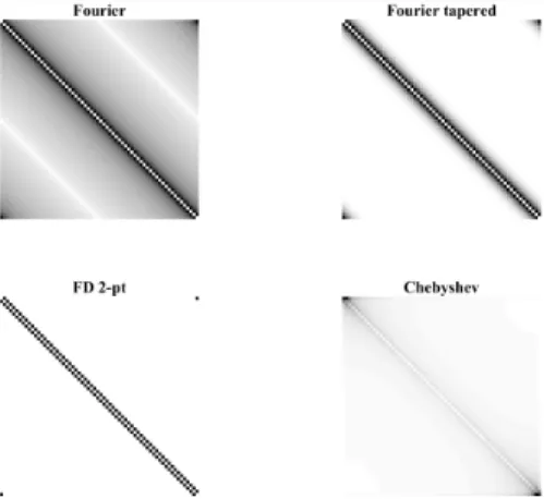
Illustration of differentiation ma- trices (n=64). Top left: Ex- act Fourier differentiation matrix for regular grid (full). Top right:

Exact Chebyshev differentiation matrix for Chebyshev collocation points. Increasing weights at the corners overshadows interior val- ues. Bottom Left: Standard 2-point finite difference operator (banded). Bottom Right: Ta- pered Fourier operator (12-point).

Matrix is banded. For illustration purposes the square root of the absolute values are shown.

23

Chebyshev Derivatives, Differentiation matrices

By testing the differentiation, we define a function to seismic wavefield calculations as

f (x

) = sin(2x

) − sin(3x

) + sin(4x

) − sin(10x

)

in the interval x

∈ [−1, 1], where the discrete

points are the Chebyshev collocation points x

=

cos(πi/n), i = 0, . . . , n given for n = 63.

Elastic 1D with Chebyshev Method

Elastic 1D with Chebyshev Method

Elastic 1D wave equation using the standard 3-point operator ρ

u

− 2u

+ u

dt

= (∂

[µ(x )∂

u(x , t)])

+ f

where the lower index i corresponds to the spatial discretization and the upper index j to the discrete time levels.

The displacement field as well as the geophysical parameters like density ρ

and

shear modulus µ

are defined on the irregular Chebyshev collocation points.

Example

• Distance between grid points is 80 times smaller at the boundaries

• The time step for a stable simulation requires cdt/dx ≤

⇒ Grid distance near boundary is responsible for the global simulation time step

Parameter Value

nx 200

c 3000 m/s

ρ 2500 kg/m

dt 6 ×10

s

dx

1.2 ×10

m dx

0.015 m

f

100 kHz

1.4

26

Result

% Time extrapolation

% for i = 1:nt,

%

% (...)

% Space derivatives du=D*u’; du=mu./rho.*du;

du=D*du;

% (...)

% Time extrapolation unew=2*u-uold+du’*dt*dt;

% Source injection

unew=unew+gauss./rho*src(i)*dt*dt;

% remapping uold=u;

u=unew;

% (...) end

Result

• To obtain a stable solution we need a very small time step that is only needed at the boundaries. Mathematically the time step scales with O(N

).

• In principle we can stretch the spatial grid such that the grid points close to the boundaries are further apart while the grid point distances at the centre remain basically unchanged. If that stretching function is ξ(x ) then the derivative of a function f (x ) on the stretched grid is defined as

∂

f (x ) = ∂f

∂ξ dξ dx .

28

Summary

• Pseudospectral methods are based on discrete function approximations that allow exact interpolation at so-called collocation points. The most prominent examples are the Fourier method based on trigonometric basis functions and the Chebyshev method based on Chebyshev polynomials.

• The Fourier method can be interpreted as an application of discrete Fourier series on a regular-spaced grid. The space derivatives can be obtained exactly (except for rounding errors). Derivatives can be efficiently calculated with the discrete Fourier transform requiringnlognoperations.

• The Fourier method implicitly assumes periodic behavior. Boundary conditions like the free surface or absorbing behaviour are difficult to implement.

• The Chebyshev method is based on the description of spatial fields using Chebyshev polynomials defined in the interval[−1,1](easily generalized to arbitrary domain sizes). Exact interpolation is possible when the discrete fields are defined at the Chebyshev collocation points given byx_i=cos(πi/n),i=0, . . . ,n.

Therefore, the derivatives can also be evaluated exactly and errors accumulate only due to the finite-difference time extrapolation.

Summary

• Because of the grid densification at the boundaries of the Chebyshev collocation points very small time steps are required for stable simulations whennis large. This can be avoided by stretching the grids by a coordinate transformation.

• A main advantage of the Chebyshev method is an elegant formulation of boundary conditions (free surface or absorbing) through the definition of so-called characteristic variables.

• Pseudospectral methods have isotropic errors. Therefore they lend themselves to the study of physical anisotropy.

• The derivative operations of pseudospectral methods are of a global nature. That means every point on a spatial grid contributes to the gradient. While this is the basis for the high precision, it creates problems when implementing pseudospectral algorithms on parallel computers with distributed memory architectures. As communication is usually the bottleneck, efficient and scalable parallelization of pseudospectral methods is difficult.

30