√ s = 8 TeV with the ATLAS detector

(1)

ATLAS-CONF-2013-058 25/08/2013

ATLAS NOTE

ATLAS-CONF-2013-058

Revised August 24, 2013

A search for heavy long-lived sleptons using 16 fb

⁻¹

of pp collisions at

√ s = 8 TeV with the ATLAS detector

The ATLAS Collaboration

Abstract

A search for heavy long-lived scalar leptons (sleptons) through a measurement of the mass of slepton candidates is presented in this note. The search is performed on a data sample of 15.9 fb⁻¹ of proton-proton collisions at a centre-of-mass energy √

s = 8 TeV collected by the ATLAS detector at the LHC in 2012. Such sleptons are expected to interact as if they were heavy muons, charged and penetrating. Their mass is estimated from a measurement of their speed,β, and their momentum,p, using the relationm= p/βγ, based on their interactions in the inner detector, the calorimeters and the muon spectrometer. No excess is observed above the estimated background. Results are interpreted in the context of gauge-mediated supersymmetry breaking (GMSB) models where the ˜τ1, supersymmetric partner of theτlepton, is the next to lightest supersymmetric particle and decays outside the ATLAS volume. Lower limits, at 95% confidence level, are set on the mass of the long-lived sleptons. Long-lived ˜τ1s in the GMSB model considered are excluded at 95% confidence level at masses below 402–347 GeV, for tanβ=5–50. Exclusion limits on the ˜τ₁mass up to 342 (300) GeV are set in the hypothesis that ˜τ₁are produced directly or via light slepton (˜e, µ) pair production, assuming a mass splittings between light slepton and stau of 1 (90) GeV.˜ In decoupled scenarios, where ˜τ₁ pair production is the only SUSY signature, exclusion limits up to 267 GeV are set on the ˜τ₁ mass. Finally, indirect constraints are placed on the mass of charginos and neutralinos.

The following have been revised with respect to the version dated June 21, 2013:

The theoretical cross-sections were re-caluclated due to a Prospino bug fix; in Figure 3 the signal has been re-normalized. Theoretical cross-sections have been updated in Figures 4, 5 and 6. Mass limit values were updated in the Abstract, Results and Conclusion sections.

c

Reproduction of this article or parts of it is allowed as specified in the CC-BY-3.0 license.

(2)

1 Introduction

Heavy long-lived particles (LLPs) are predicted in a variety of theories extending the Standard Model (SM). In Supersymmetry (SUSY) [1–9], sleptons (˜l, superpartners of leptons), squarks and gluinos ( ˜q, g, superpartners of quarks and gluons, respectively) might have long lifetimes and decay outside the˜ detector volume. Heavy LLPs produced at the Large Hadron Collider (LHC) could travel with velocity measurably lower than the speed of light. These particles can be identified and their mass,m, determined from their velocity,β, and momentum,p, using the relationm= p/βγ.

Long-lived charged sleptons would interact like heavy muons, releasing energy by ionisation as they pass through the ATLAS detector. A search for long-lived sleptons identified in the inner detector (ID), calorimeter and the muon spectrometer (MS), is therefore performed. The results are interpreted in the framework of gauge-mediated SUSY breaking (GMSB) [10–16] with the light stau (˜τ₁) as the LLP.

In GMSB models, either the sleptons or the neutralino are the next to lightest supersymmetric particle (NLSP). The GMSB model parameters for this search are chosen such that ˜τ₁is the NLSP and the scale factor for the gravitino mass, which determines the NLSP life time, is chosen to ensure that the NLSP does not decay in the detector. The ˜τ₁, the lightest ˜τmass eigenstate resulting from the mixture of right- handed and left-handed superpartners of theτlepton, is the long-lived NLSP. The ˜τ₁is predominantly right handed in all models considered here. The mass splitting with the other sleptons is small but ˜τ1is always the NLSP.

A search for long-lived sleptons is presented in this note using time-of-flight and specific ionisation energy loss, dE/dx, to measureβ. The background is primarily composed of high-p_T muons with mis- measuredβorβγ. It is estimated directly from the same data sample by convoluting the momentum and βdistributions of the LLP candidates.

The analysis divides the events into two regions: events with two selected candidates and events with one selected candidate. A loose selection with high signal efficiency is used to select candidates in events where there are two LLP candidates. In events where only one candidate passes the loose selection, that candidate is required to pass an additional, tighter selection. The one candidate sample is used to assess systematic uncertainties on the background estimate.

Previous collider searches for LLPs have been performed at LEP [17–20], HERA [21], the Tevatron [22–

28], and the LHC [29–37].

2 The ATLAS detector

The ATLAS detector [38] is a multipurpose particle physics detector with a forward-backward symmet- ric cylindrical geometry and near 4πcoverage in solid angle¹. The ID consists of a silicon pixel detector, a silicon micro-strip detector, and a straw tube transition radiation tracker. The ID is surrounded by a thin superconducting solenoid providing a 2 T magnetic field, and by high-granularity liquid-argon sampling electromagnetic calorimeters. A steel scintillator tile calorimeter provides hadronic coverage in the cen- tral rapidity range. The end-cap and forward regions are instrumented with liquid-argon calorimetry for both electromagnetic and hadronic measurements. The MS surrounds the calorimeters and consists of three large superconducting air-core toroids each with eight coils, a system of precision tracking cham-

1ATLAS uses a right-handed coordinate system with its origin at the nominal interaction point in the centre of the detector and thez-axis coinciding with the axis of the beam pipe. Thex-axis points from the interaction point to the centre of the LHC ring, and they-axis points upward. Cylindrical coordinates (r,φ) are used in the transverse plane,φbeing the azimuthal angle around the beam pipe. The pseudo-rapidity is defined in terms of the polar angleθasη=−ln tan(θ/2).

(3)

bers, and detectors for triggering.

ATLAS has a trigger system designed to reduce the data taking rate from up to 40 MHz to about 400 Hz, and keep the events that are potentially the most interesting. The first-level trigger (level-1) selection is carried out by custom hardware and identifies detector regions and a bunch crossing for which a trigger element is found. The high-level trigger is performed by dedicated software, seeded by data acquired from the bunch crossing and regions found at level-1. The components of particular importance to this analysis are described in more detail below.

3 Data and simulated samples

The work presented in this note is based on 15.9±0.45 fb⁻¹ofppcollision data collected in 2012. The events are selected online by muon triggers. Data and simulated (MC)Z →µµsamples are used forβ resolution studies. Simulated signal samples are used to study the expected signal behaviour and to set limits.

The GMSB samples are generated with the following model parameters: number of super-multiplets in the messenger sector, N₅ = 3, messenger mass scale,m_messenger = 250 TeV, sign of the Higgsino mass parameter, sign(µ) = 1, and C_grav, the scale factor for the gravitino mass which determines the NLSP lifetime is set to 5000 to ensure that the NLSP does not decay in the detector. The two Higgs doublets vacuum expectation values ratio, tanβ, is varied between 5 and 50. The SUSY breaking scaleΛis varied from 80 to 160 TeV and the corresponding ˜τ₁masses vary from 175 to 510 GeV. The masses of the right handed ˜e(or ˜µ) are larger than that of ˜τ₁by 0.75–90 GeV for tanβvalues from 5 to 50. The corresponding light neutralino masses vary from 328 GeV to 709 GeV as a function ofΛand are independent of tanβ, the chargino masses vary from 540 GeV to 940 GeV, 210 to 260 GeV higher than the neutralino masses, with a small dependence on tanβthat varies from 1% atΛ =80 TeV to 3% atΛ =80 TeV.

The mass spectra of the GMSB models are obtained from the Spice program [39] and the events are generated using Herwig [40]. Cross-sections at NLO accuracy obtained with Prospino[41] are used.

The production cross-section at these masses is dominated by direct di-slepton production, while the second largest contribution is from ˜χ⁰₁χ˜⁺₁ production.

All simulated events pass the full ATLAS detector simulation [42,43] and are reconstructed with the same programs as the data. Pile-up of collisions, simulating the conditions in 2012 data taking, is included in the simulation. All signal samples are normalised to the integrated luminosity of the data.

4 The β measurement

4.1 The pixel detector

As the innermost sub-detector in ATLAS, the silicon pixel detector provides at least three precision measurements for each track in the region |η| < 2.5 at radial distances from the LHC beam line R <

15 cm. The time for which the signal is above threshold (ToT) provides a measurement of the deposited charge. Neighbouring pixels are joined together to form clusters and the charge of a cluster is calculated by summing up the charges of all pixels after applying a correction obtained from calibration. The specific energy loss dE/dx, defined as an average of the individual cluster charge measurements for the clusters associated with the track, is used to calculate β. To reduce the Landau tails, the average is evaluated after having removed the cluster with the highest charge (the two clusters with the highest

(4)

charge are removed for tracks having five or more clusters). The measurableβγrange lies between 0.2 and 1.5, the lower bound being defined by the overflow in the ToT spectrum, and the upper bound by the overlapping distributions in the relativistic rise branch of the curve. This particle identification method, described in Ref. [44], uses a five-parameter function to describe how the most probable value of the specific energy loss (MdE

dx) depends onβγ:

MdE

dx(βγ)= p₁

β^p³ ln(1+(p₂βγ)^p⁵)−p₄ (1) 4.2 Calorimeters

Liquid argon is used as the active detector medium in the electromagnetic (EM) barrel and end-cap calorimeters, as well as in the hadronic end-cap (HEC) calorimeter. All are sampling calorimeters, using lead plates for the EM calorimeters and copper plates for the HEC calorimeter. The ATLAS tile calorimeter is a cylindrical hadronic sampling calorimeter. It uses steel as absorber material and plastic scintillators as the active layers, with ηcoverage to|η| . 1.7. The calorimeters are segmented in cells transverse to the particle paths and layers along the particle paths.

The ATLAS tile and LAr calorimeters have sufficiently good timing resolutions to distinguish highly relativistic SM particles from the slower moving LLPs. The time resolution depends on the energy deposited in the cell and also the layer type and thickness, but typical resolutions are 2 ns for an energy deposit of 1 GeV, and generally better for the tile calorimeter.

4.3 The muon detectors

The MS forms the outer part of the ATLAS detector and detects charged particles exiting the calorimeters and measures their momenta in the pseudo-rapidity range |η| < 2.7. It is also designed to trigger on these particles in the region |η| < 2.4. The chambers in the barrel are arranged in three concentric cylindrical shells around the beam axis while in the two end-cap regions, muon chambers form large wheels, perpendicular to thez-axis.

The precision momentum measurement is performed by monitored drift-tube (MDT) chambers, using theη coordinate. These chambers consist of three to eight layers of drift tubes. In the forward region (2 < |η| < 2.7), Cathode-Strip Chambers are used in the innermost tracking layer. Resistive plate chambers (RPC) in the barrel region (|η|<1.05), and thin gap chambers in the end-cap (1.05<|η|<2.4), deliver a fast level-1 trigger and measure both coordinates of the track,ηandφ.

The default reconstruction of particles in the MDT [45] relies on the assumption that they travel with the speed of light (β = 1). To improve the track quality for slow LLPs, the individual track segments are reconstructed with different values for β. The actual β of the particle is estimated from the set of segments with the lowestχ². In a successive combined track re-fit, including ID and MS hits, the particle trajectory is estimated more accurately. The time of flight to each tube is then obtained using the difference between the re-fitted track position in each tube and the radius calculated assumingβ=1. By averaging theβs estimated from the time of flight in the different tubes an improved MDTβestimation is achieved.

The RPC have an intrinsic time resolution of∼1 ns while the digitised signal is sampled with a 3.12 ns granularity, allowing a measurement of the time of flight. In the RPC,βis first calculated separately for

(5)

each hit from the independent position and time measurements. A single β estimation is obtained by averaging theβs from all the hits.

4.4 Calibrating time measurements

To ensure the highest possible timing accuracy, it is necessary to calibrate the data using particles with known speed. It is then possible to correct the time-of-flight (ToF) values such that they are in agreement with the known values. The ToF measurement is sensitive to relative offsets in the time calibration between the different detector elements. By definition, in a perfectly calibrated detector, an energetic muon coming from a collision at the interaction point will traverse the detector att₀ = 0. Thet₀distributions in the different detector elements are measured for muons from data. The means of the distributions are used to correct the calibration by shifting the measuredt₀s, and their widths are used as the resolution of the time measurement in theβ⁻¹average.

The t₀ distributions are also extracted from aZ → µµMC sample and compared with those found in data. In order to simulate the actual detector conditions in the MC, time measurements are smeared to the widths found in data.

4.5 Combiningβmeasurements

Theβmeasurements from the different detectors are only used ifβ >0.2 (the limit of the fit at reconstruction) and if they are consistent internally, i.e. theχ²probability of the average between hits is reasonable (calorimeter) or the RMS of the measurement is consistent with the expected errors (MS). Measurements that are accepted are combined in a weighted average. The weights are obtained from the calculated error of each measurement. The pixel ToT is required to be consistent with other measurements but is not included in the average.

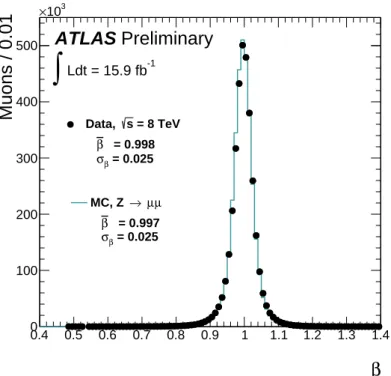
Sinceβ is estimated from the measured time of flight, for a given resolution on the time measurement, a slower particle has a better β resolution. Figure 1 shows the β distribution for selected muons (as described in 5.2) in data andZ → µµdecays in MC simulation with smeared hit times. The smearing mechanism reproduces the measured muonβdistribution to a satisfactory level. The same time-smearing mechanism is applied to the signal MC samples.

5 Event and candidate selection

5.1 Trigger selection

This analysis is based on events collected using un-prescaled single muon triggers with ap_Tthreshold of 24 GeV. Offline muons are selected withp_T >50 GeV, well above the trigger threshold. Level-1 muon triggers are accepted and passed to the high-level trigger only if assigned to the collision bunch crossing.

Late triggers due to late arrival of the particles are thus lost. The trigger efficiency for particles arriving late at the muon spectrometer is difficult to assess from data, where the majority of candidates are in-time muons. This efficiency is obtained from simulated GMSB events passing the Level-1 trigger simulation.

The muon triggers are found to be efficient for GMSB signatures, which contain two LLPs that reach the MS, and additional muons stemming from neutralino decays. The estimated trigger efficiency depends on the signal processes considered: it is found to be between 65% and 82% for inclusive GMSB slepton

(6)

β

0.4 0.5 0.6 0.7 0.8 0.9 1 1.1 1.2 1.3 1.4

Muons / 0.01

0 100 200 300 400 500

103

×

ATLAS Preliminary

= 8 TeV s Data,

= 0.998 β

= 0.025 σβ

µ µ

→ MC, Z

= 0.997 β

= 0.025 σβ

Ldt = 15.9 fb-1

∫

Figure 1: Distribution of the combinedβmeasurement for selected muons in data andZ →µµdecays in MC simulation. The typical resolutions are 0.025.

production, between 61% and 78% for direct slepton production and between 69% and 85% for chargino and neutralino production events.

5.2 Offline selection

Event selection

Collision events are selected by requiring a good primary vertex, with at least three ID tracks, and with requirements on the position of the reconstructed primary vertex. The primary vertex is defined as the reconstructed vertex with the highestP

p²_T of associated tracks. Events flagged as having flaws in detector operation are rejected. This analysis requires at least two loosely identified muons in each event, because ˜τ₁s are expected to be produced in pairs, either via direct production or as decay product of high- mass pair produced sparticles, and both with a high probability of being observed in the MS. Cosmic ray background is rejected by removing tracks that do not pass close to the primary vertex inz. Candidates with an ID track with|z^trk₀ −z^vtx₀ | > 10 mm are removed, wherez^trk₀ is the zcoordinate at the distance of closest approach of the track to the primary vertex. Events with cosmic rays are also rejected by a topological cut on any two candidates with oppositeηandφ(|η₁+η₂|<0.005 and||φ₁−φ₂| −π|<0.005).

LLP candidate selection

Two sets of selection criteria are applied. A loose selection with high efficiency is used to select candidates in events where there are two LLP candidates. Very rarely would a non-GMSB event have two high p_Tmuons, both withβfrom the tail of the distribution and a large reconstructed mass. In events where only one candidate passes the loose selection, that candidate is required to pass a tighter selection.The one tight candidate sample is used for background estimation checks.

LLP candidates in the loose slepton selection are required to have p_T >50 GeV. Thep_Tmeasurements

(7)

in the ID and MS are required to be consistent, and the difference between them should not exceed a half of their average. Each candidate is required to have |η| < 2.5. Any two candidates that combine together to give an invariant mass close to theZmass (±10 GeV) are both rejected. Candidates are also required to have associated hits in at least two different muon stations. The estimated βis required to be consistent between measurements in the same sub-detector, based on the hit time resolutions. The calorimeterβ χ² probability is required to be greater than 0.001 and the RMS of the RPC and MDTβ measurements is required to be less than 0.3. The number of calorimeter cells and MS hits contributing to theβmeasurement must exceed the number of detector systems used by three. For signal, lowβvalues should be correlated between measurements whereas for muons they are the result of poor estimation and should be uncorrelated between measurements. Therefore theβ measurements from the different sub- detectors are required to be consistent with each other. Theβs measured in each sub-detector separately are required to be within 3σfrom one another, and the combinedβto be consistent with theβγestimated in the pixel within 3σ. Finally, in order to reject muons, the combinedβmeasurement is required to be less than 0.95.

To pass the tight selection, a candidate is required in addition to havep_T>70 GeV, at least two separate sub-detectors measuringβ, the number of calorimeter cells and MS hits contributing to theβ measurement must exceed the number of detector systems used by at least twelve, and the consistency betweenβ estimates in different sub-detectors must be within 2σ. These cuts are optimised to give very high quality βmeasurements and thus reduced backgroundβbelow 0.95.

Finally, a lower mass cut is applied on the candidate measured mass,m_β= p/βγ. For the two candidate sample, both masses are required to be above the cut. The cut value depends on the hypothetical ˜τ₁ mass and is different for different GMSB models. It is chosen to accept 99% of the reconstructed signal mass for each model. The cut value ranges from 120 GeV for a ˜τ₁mass of 175 GeV to 320 GeV for a τ˜₁ mass of 500 GeV. The number of background and expected signal events above the mass cut in the two-candidate signal region is used to obtain the exclusion limit.

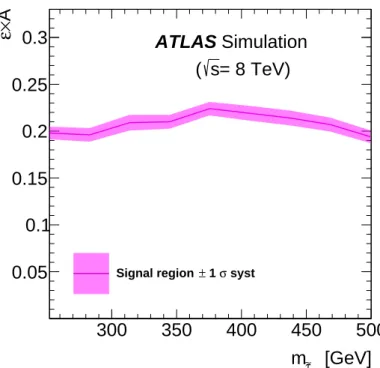
Figure 2 shows the selection efficiency for the directly produced sleptons as a function of their mass.

Typical efficiencies for signal passing the mass cuts are 20% for the two candidate events and 15% for the one candidate events, and similar for all production processes. Despite the high efficiency of the one candidate region, the relative amount of signal with respect to background is very low with respect to the two candidate region, but it can be used to validate the background estimation methods.

6 Background estimation

The background to this search is mostly composed of high-pTmuons with mis-measuredβand is estimated directly from data. The estimation of the background mass distributions relies on two premises:

that the signal to background ratio before applying cuts on β is small, and that the β distribution for background candidates is due to measurement resolution and is therefore independent of the source of the candidate and its momentum.

The detector is divided intoηregions so that theβresolution within each region is similar. The muon-β probability density function (PDF) in each ηregion is the distribution of the measured βof all muons in the region. For each candidate a random β is drawn from the muon-β PDF in its region. If this β passes the selection, a mass is calculated using the reconstructed momentum of the candidate and the randomβ. The statistical fluctuations in the background estimate are reduced by repeating the procedure many times for each candidate and dividing the resulting distribution by the number of repetitions. This procedure is self-normalizing and no further normalization of the background estimate to data is applied.

(8)

[GeV]

τ∼1

m

300 350 400 450 500

A×ε

0.05 0.1 0.15

0.2 0.25

0.3 ATLAS Simulation

= 8 TeV) s

(

syst σ

± 1 Signal region

Figure 2: Efficiency times acceptance for directly produced slepton events in the two-candidate signal region as a function of the ˜τ₁mass.

The reconstructed mass distribution of muons in different regions of the detector depends on bothβand momentum distributions through m = p/βγ. The regions also differ in the muon momentum distribution, therefore the combination of momentum with randomβis done separately in each region and the resulting mass distributions are added together. The distribution of mass obtained this way represents the background estimate.

7 Systematic uncertainties

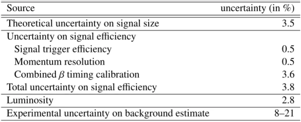
Several possible sources of systematic effects are studied. The resulting systematic uncertainties are summarised in Table 1.

Theoretical cross-sections

The nominal signal NLO cross-section and its uncertainty are taken from the envelope of cross-section predictions using different parton distribution function sets, factorisation and renormalisation scales, as described in Ref. [46]. This prescription leads to a 3.5% relative uncertainty on the expected signal normalisation. The systematic is small because the search is dominated by electro-weak production.

Expected signal

The muon trigger efficiency for muons is calculated using the tag-and-probe technique onZ→µµevents as described in Ref. [47]. The uncertainty on the single muon trigger efficiency is estimated to be 0.5%.

The effect of a late arriving particle on the trigger efficiency, estimated using the trigger simulation, depends on the exact timing implementation in the simulation. Since the trigger simulation is performed on unsmeared hit times, while the actual trigger is performed on uncalibrated time measurements, we emulated the procedure as follows. The muon trigger efficiency curve has been extracted as a function

(9)

Source uncertainty (in %)

Theoretical uncertainty on signal size 3.5

Uncertainty on signal efficiency

Signal trigger efficiency 0.5

Momentum resolution 0.5

Combinedβtiming calibration 3.6

Total uncertainty on signal efficiency 3.8

Luminosity 2.8

Experimental uncertainty on background estimate 8–21

Table 1: Summary of systematic uncertainties (given in percent). Where a range is given it corresponds to different mass hypotheses (low-high mass).

ofβfrom MC signal samples; the MC hit time distribution in the RPC has been smeared in order to re- produce the corresponding data distribution by adding the strip-by-strip shifts of the hit time distribution observed in data, electronic and charge jitter; the trigger efficiency curve has been applied to the smeared MC and the trigger efficiency has been re-evaluated. Since the efficiency obtained by this procedure is higher than that obtained using the trigger simulation, no systematic uncertainty is assigned to the trigger efficiency evaluated by using the standard simulation.

The systematic uncertainty due to the track reconstruction efficiency and momentum resolution differences between ATLAS data and simulation are estimated [48] to be 0.5% for GMSB events.

The signalβ resolution is estimated by smearing the hit times according to the spread observed in the time calibration. The systematic uncertainty due to the smearing process is estimated by scaling the smearing factor up and down, so as to bracket the distribution obtained in data. A 3.6% systematic uncertainty is found for the two-candidate GMSB signal region and the corresponding uncertainty for the one-candidate region used for background systematic estimation is 4.1%

The uncertainty on the integrated luminosity is 2.8%. It is derived, following the same methodology as that detailed in Ref. [49], from a preliminary calibration of the luminosity scale derived from beam- separation scans performed in November 2012.

Background estimation

The uncertainty on the background estimation is derived from the difference between data and background estimate observed in the one candidate region, and the statistical error on it. The fractional uncertainty obtained this way is assigned to each bin in the two candidate background estimate. The procedure assumes that signal contamination in the one candidate region is negligible compared to that of the two candidate region, and that the uncertainty factorises between the two heavy slepton candidates. It also neglects possible differences between the loose and tight selections in the uncertainty determination.

The resulting uncertainty in the total background estimate above the mass cut applied for each model ranges between 8% and 21%.

8 Results

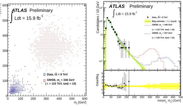
The mass distributions observed in data together with the background estimate, its systematic uncertainty and examples of signal are shown in Figure 3, for the two-candidate signal region. The two signal

(10)

[GeV]

m1

0 100 200 300 400 500 600

[GeV]2m

0 100 200 300 400 500 600

= 8 TeV s Data,

= 346 GeV GMSB, mτ∼

= 10) β = 110 TeV, tan Λ

(

ATLAS Preliminary Ldt = 15.9 fb-1

∫

) [GeV]

, m2

min(m1

0 50 100 150 200 250 300 350 400 450 500

Candidates / 10 GeV

10-1 1 10 102

103 ATLAS Preliminary

Ldt = 15.9 fb-1

∫

^Data,^s^{= 8 TeV}

(syst) σ

± 1 Bkg estimate

= 346 GeV τ∼1

GMSB, m = 10) β = 110 TeV, tan Λ (

= 437 GeV τ∼1

GMSB, m = 10) β = 140 TeV, tan Λ (

) [GeV]

, m2

min(m1

0 50 100 150 200 250 300 350 400 450 500

Data/Bkg

-1 0 1 2 3 4 5

Figure 3: On the left, observed data and expected signal in the two-candidate signal region in the slepton search. On the right, the lower of the two masses is plotted for observed data, background estimate and expected signal for ˜τ₁masses of 346 GeV and 437 GeV.

samples shown on the right have ˜τ₁masses of 346 GeV and 437 GeV.

No indication of signal above the expected background is observed, and limits on new physics scenarios are set. Cross-section limits are obtained using theCLs prescription [50]. Mass limits are derived by comparing the obtained cross-section limits to the lower edge of the 1σ band around the theoretically predicted cross-section for each process.

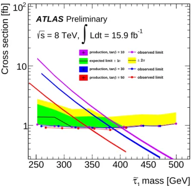
The resulting production cross-section limits at 95% confidence level (CL) in the GMSB scenario as a function of the ˜τ₁mass are presented in Figure 4 and compared to theoretical predictions. A long-lived τ˜1in GMSB models withN₅ =3,m_messenger = 250 TeV and sign(µ) = 1 are excluded at 95% CL up to masses of 391, 402, 392, 382, 366, 347, GeV for tanβ=5, 10, 20, 30, 40 and 50, respectively.

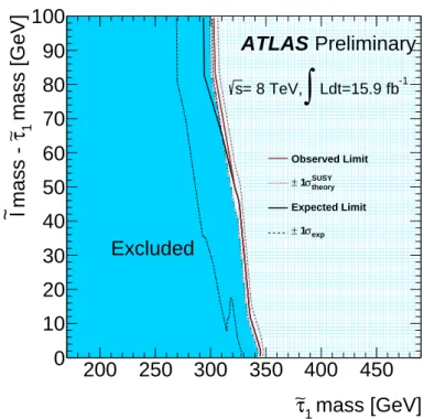
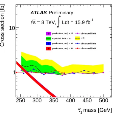
Limits on the rates of specific production mechanisms are obtained by repeating the analysis on subsets of the GMSB samples corresponding to each production mode. For GMSB models with parameters in this range, strong production of squarks and gluinos is suppressed due to their large masses. Directly produced sleptons comprise 30–63% of the GMSB cross-section, and the corresponding ˜τ₁ production rates depend only on the ˜τ₁ mass and the mass difference between the right handed ˜e (or ˜µ) and the τ˜₁. Thus, using the same analysis, constraints can be made on a simple model with only pair-produced sleptons which are long lived, or which themselves decay to long-lived sleptons of another flavour. Such direct production is excluded at 95% CL up to ˜τ₁ masses of 342 to 300 GeV for models with slepton mass splittings of 0.75 to 90 GeV. The slepton direct production limits are shown in Figure 5. Figure 6 shows the cross-section limits on direct ˜τ₁production, as would be the case when the mass splitting to the other sleptons is very large. Masses below 267 GeV are excluded if only ˜τ₁is produced.

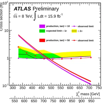
Finally, in the context of the GMSB model, 30–50% of the GMSB cross-section arises from direct production of charginos and neutralinos (dominated by ˜χ⁰₁χ˜⁺₁ production) and subsequent decay to ˜τ₁.

(11)

Figure 7 shows the 95% CL lower limits on the ˜χ⁰and ˜χ⁺mass when the final decay product is a long- lived ˜τ₁². ˜χ⁰ masses below 475–490 GeV are excluded, with corresponding ˜χ⁺ masses 210–260 GeV higher.

mass [GeV]

τ∼1

250 300 350 400 450 500

Cross section [fb]

1 10 102

= 10 β production, tan

σ

± 1 expected limit

observed limit σ

± 2 observed limit observed limit

Ldt = 15.9 fb-1

∫

= 8 TeV, s

Figure 4: Cross-section limits as a function of the ˜τ₁mass in GMSB models. Observed limits are given as solid lines with markers. The theoretical prediction for the cross-section is shown as a colored 1σ band. Different colors represent models with different tanβ. Expected limits for tanβ= 10 are drawn as black lines with±1 and±2σuncertainty bands drawn in green and yellow respectively.

9 Conclusion

A search for heavy long-lived sleptons through measurement of the mass of slepton candidates by means of time-of-flight and specific ionisation loss measurements in ATLAS subdetectors has been performed.

The data are found to match the Standard Model background expectation in all signal regions. The exclusion limits placed for various models impose new constraints on non-SM cross-sections. Long-lived τ˜₁s in the GMSB model considered are excluded at 95% CL at masses below 402–347 GeV, for tanβ= 5–50. Directly produced long-lived sleptons are excluded below 342 GeV for small mass difference between the light (right handed) sleptons and the ˜τ₁, and below 300 GeV for mass splittings of 90 GeV.

If only ˜τ₁is produced, its mass is excluded below 267 GeV. Neutralinos that decay to long-lived ˜τs are excluded below 475 GeV.

These results, thanks to increased luminosity and more advanced data analysis, substantially extend our previous limits [36], and are largely complementary to the searches for SUSY particles decaying promptly.

2The mass of the ˜τ1decreases with increasing tanβand increases with the ˜χ⁰and ˜χ⁺masses. At low ˜χ⁰and ˜χ⁺masses and large tanβ, the cross-section limits are thus affected by the amount of background in the ˜τ1mass search region, which starts at 120 GeV for tanβ=50 and at 170 GeV for tanβ=10.

(12)

mass [GeV]

τ∼1

200 250 300 350 400 450 mass [GeV] 1τ∼ mass - l~

0 10 20 30 40 50 60 70 80 90 100

= 8 TeV,

s

∫

Ldt=15.9 fb^-1

Excluded

Observed Limit

theory

σSUSY

± 1

Expected Limit

σexp

± 1

Figure 5: Excluded regions for directly produced sleptons in the plane m(˜l)− m(˜τ₁) vs. m(˜τ₁). The excluded region is blue. The three red lines correspond to the limit with the theoretical prediction±1σ.

The kink in the lower uncertainty contour of the expected limit is a drawing feature due to the limited density of simulated grid points.

References

[1] H. Miyazawa, Prog. Theor. Phys.36 (6)(1966) 1266–1276.

[2] P. Ramond, Phys. Rev.D3(1971) 2415–2418.

[3] Y. A. Gol’fand and E. P. Likhtman, JETP Lett.13(1971) 323–326. [Pisma Zh.Eksp.Teor.Fiz.13:452-455,1971].

[4] A. Neveu and J. H. Schwarz, Nucl. Phys.B31(1971) 86–112.

[5] A. Neveu and J. H. Schwarz, Phys. Rev.D4(1971) 1109–1111.

[6] J. Gervais and B. Sakita, Nucl. Phys.B34(1971) 632–639.

[7] D. V. Volkov and V. P. Akulov, Phys. Lett.B46(1973) 109–110.

[8] J. Wess and B. Zumino, Phys. Lett.B49(1974) 52.

[9] J. Wess and B. Zumino, Nucl. Phys.B70(1974) 39–50.

[10] M. Dine and W. Fischler, Phys. Lett.B110(1982) 227.

[11] L. Alvarez-Gaume, M. Claudson, and M. B. Wise, Nucl. Phys.B207(1982) 96.

[12] C. R. Nappi and B. A. Ovrut, Phys. Lett.B113(1982) 175.

(13)

mass [GeV]

τ∼1

250 300 350 400 450 500

Cross section [fb]

1 10

σ

± 2 observed limit observed limit

ATLAS Preliminary = 8 TeV,

s

∫

Ldt = 15.9 fb^-1

Figure 6: Cross-section limits as a function of the ˜τ₁ mass for direct ˜τ₁ production. Expected limits are drawn as black lines with ±1 and ±2σuncertainty bands drawn in green and yellow respectively.

Observed limits are given as markers. The theoretical cross-section prediction is shown as a colored 1σ band.

[13] M. Dine and A. E. Nelson, Phys. Rev.D48(1993) 1277–1287.

[14] M. Dine, A. E. Nelson, and Y. Shirman, Phys. Rev.D51(1995) 1362–1370.

[15] M. Dine, A. E. Nelson, Y. Nir, and Y. Shirman, Phys. Rev.D53(1996) 2658–2669.

[16] C. F. Kolda, Nucl. Phys. Proc. Suppl.62(1998) 266–275.

[17] ALEPH Collaboration, R. Barate et al., Phys.Lett.B405(1997) 379–388.

[18] DELPHI Collaboration, P. Abreu et al., Phys.Lett.B478(2000) 65–72.

[19] L3 Collaboration, P. Achard et al., Phys.Lett.B517(2001) 75–85.

[20] OPAL Collaboration, G. Abbiendi et al., Phys.Lett.B572(2003) 8–20.

[21] H1 Collaboration Collaboration, A. Aktas et al., Eur.Phys.J.C36(2004) 413–423.

[22] CDF Collaboration, F. Abe et al., Phys.Rev.Lett.63(1989) 1447.

[23] CDF Collaboration, F. Abe et al., Phys.Rev.D46(1992) 1889–1894.

[24] CDF Collaboration, D. Acosta et al., Phys.Rev.Lett.90(2003) 131801.

[25] D0 Collaboration, V. M. Abazov et al., Phys. Rev. Lett.99(2007) 131801.

[26] D0 Collaboration, V. Abazov et al., Phys.Rev.Lett.102(2009) 161802.

(14)

mass [GeV]

1

χ∼0

300 350 400 450 500 550 600 650 700 750

Cross section [fb]

10-1

1 10 102

σ

± 2

observed limit

Ldt = 15.9 fb-1

∫

= 8 TeV, s

mass [GeV]

1

χ∼+

550 600 650 700 750 800 850 900 950

Figure 7: Cross-section limits as a function of the ˜χ mass for ˜τ₁s from chargino and neutralino production. Observed limits are given as solid lines with markers. Different colors represent models with different tanβ. Expected limits for tanβ = 10 are drawn as black lines with ±1 and ±2σ uncertainty bands drawn in green and yellow respectively. The theoretical cross-section prediction (dominated by χ˜⁰₁χ˜⁺₁ production) is shown as a colored 1σband.

(15)

[27] CDF Collaboration, T. Aaltonen et al., Phys.Rev.Lett.103(2009) 021802.

[28] D0 Collaboration, V. M. Abazov et al., Phys. Rev. Lett.108(2012) 121802.

[29] CMS Collaboration, Phys.Rev.Lett.106(2011) 011801.

[30] CMS Collaboration, JHEP1103(2011) 024.

[31] ATLAS Collaboration, Phys.Lett.B698(2011) 353–370.

[34] ATLAS Collaboration, Eur.Phys.J.C72(2012) 1965.

[35] CMS Collaboration, Phys.Lett.B713(2012) 408–433.

[37] CMS Collaboration,arXiv:1305.0491 [hep-ex].

[38] ATLAS Collaboration, JINST3(2008) S08003.

[39] G. Engelhard, J. L. Feng, I. Galon, D. Sanford, and F. Yu, Comput.Phys.Commun.181(2010) 213–226.

[40] G. Corcella et al., JHEP01(2001) 010.

[41] W. Beenakker, R. Hopker, M. Spira, and P. M. Zerwas, Nucl. Phys.B492(1997) 51–103.

[42] GEANT4 Collaboration, S. Agostinelli et al., Nucl. Instrum. Meth.A506(2003) 250–303.

[43] ATLAS Collaboration, Eur.Phys.J.C70(2010) 823–874.

[44] ATLAS Collaboration, ATLAS-CONF-2011-016 (2011), http://cds.cern.ch/record/1336519.

[45] ATLAS Collaboration, CERN-OPEN-2008-020.

[46] M. Kramer, A. Kulesza, R. van der Leeuw, M. Mangano, S. Padhi, et al.,arXiv:1206.2892 [hep-ph].

[47] T. Matsushita, ATL-DAQ-PROC-2012-008,http://cds.cern.ch/record/1455099.

[48] ATLAS Collaboration, ATLAS-CONF-2011-063,http://cds.cern.ch/record/1455099.

[49] ATLAS Collaboration, submitted to Eur. Phys. J. C (2013),arXiv:1302.4393 [hep-ex].

[50] A. L. Read, J. Phys. G28(2002) 2693–2704.