Measurement of |Vcb

(1)

arXiv:hep-ex/0003013v1 10 Mar 2000

OPAL PR 305 CERN-EP-2000-032 February 23, 2000

Measurement of | V

_cb

| using ¯ B

⁰

→ D

^∗+

ℓ

⁻

ν ¯ decays

The OPAL Collaboration

Abstract

The magnitude of the Cabibbo-Kobayashi-Maskawa matrix element Vcb has been measured using ¯B⁰→D^∗⁺ℓ⁻ν¯decays recorded on the Z⁰peak using the OPAL detector at LEP. The D^∗⁺→ D⁰π⁺ decays were reconstructed both in the particular decay modes D⁰ → K⁻π⁺ and D⁰ → K⁻π⁺π⁰ and via an inclusive technique. The product of |Vcb| and the decay form factor of the B¯⁰→D^∗⁺ℓ⁻ν¯transition at zero recoilF(1) was measured to beF(1)|Vcb|= (37.1±1.0±2.0)×10⁻³, where the uncertainties are statistical and systematic respectively. By using Heavy Quark Effective Theory calculations forF(1), a value of

|Vcb|= (40.7±1.1±2.2±1.6)×10⁻³

was obtained, where the third error is due to theoretical uncertainties in the value of F(1). The branching ratio Br( ¯B⁰→D^∗⁺ℓ⁻¯ν) was also measured to be (5.26±0.20±0.46) %.

Submitted to Physics Letters B.

(2)

The OPAL Collaboration

G. Abbiendi², K. Ackerstaff⁸, P.F. Akesson³, G. Alexander²², J. Allison¹⁶, K.J. Anderson⁹, S. Arcelli¹⁷, S. Asai²³, S.F. Ashby¹, D. Axen²⁷, G. Azuelos^18,a, I. Bailey²⁶, A.H. Ball⁸, E. Barberio⁸, R.J. Barlow¹⁶,

J.R. Batley⁵, S. Baumann³, T. Behnke²⁵, K.W. Bell²⁰, G. Bella²², A. Bellerive⁹, S. Bentvelsen⁸, S. Bethke^14,i, O. Biebel^14,i, A. Biguzzi⁵, I.J. Bloodworth¹, P. Bock¹¹, J. B¨ohme^14,h, O. Boeriu¹⁰, D. Bonacorsi², M. Boutemeur³¹, S. Braibant⁸, P. Bright-Thomas¹, L. Brigliadori², R.M. Brown²⁰,

H.J. Burckhart⁸, J. Cammin³, P. Capiluppi², R.K. Carnegie⁶, A.A. Carter¹³, J.R. Carter⁵, C.Y. Chang¹⁷, D.G. Charlton^1,b, D. Chrisman⁴, C. Ciocca², P.E.L. Clarke¹⁵, E. Clay¹⁵, I. Cohen²²,

O.C. Cooke⁸, J. Couchman¹⁵, C. Couyoumtzelis¹³, R.L. Coxe⁹, M. Cuffiani², S. Dado²¹, G.M. Dallavalle², S. Dallison¹⁶, R. Davis²⁸, A. de Roeck⁸, P. Dervan¹⁵, K. Desch²⁵, B. Dienes^30,h,

M.S. Dixit⁷, M. Donkers⁶, J. Dubbert³¹, E. Duchovni²⁴, G. Duckeck³¹, I.P. Duerdoth¹⁶,

P.G. Estabrooks⁶, E. Etzion²², F. Fabbri², A. Fanfani², M. Fanti², A.A. Faust²⁸, L. Feld¹⁰, P. Ferrari¹², F. Fiedler²⁵, M. Fierro², I. Fleck¹⁰, A. Frey⁸, A. F¨urtjes⁸, D.I. Futyan¹⁶, P. Gagnon¹², J.W. Gary⁴, G. Gaycken²⁵, C. Geich-Gimbel³, G. Giacomelli², P. Giacomelli², D.M. Gingrich^28,a, D. Glenzinski⁹,

J. Goldberg²¹, W. Gorn⁴, C. Grandi², K. Graham²⁶, E. Gross²⁴, J. Grunhaus²², M. Gruw´e²⁵, P.O. G¨unther³, C. Hajdu²⁹ G.G. Hanson¹², M. Hansroul⁸, M. Hapke¹³, K. Harder²⁵, A. Harel²¹,

C.K. Hargrove⁷, M. Harin-Dirac⁴, A. Hauke³, M. Hauschild⁸, C.M. Hawkes¹, R. Hawkings²⁵, R.J. Hemingway⁶, C. Hensel²⁵, G. Herten¹⁰, R.D. Heuer²⁵, M.D. Hildreth⁸, J.C. Hill⁵, P.R. Hobson²⁵,

A. Hocker⁹, K. Hoffman⁸, R.J. Homer¹, A.K. Honma⁸, D. Horv´ath^29,c, K.R. Hossain²⁸, R. Howard²⁷, P. H¨untemeyer²⁵, P. Igo-Kemenes¹¹, D.C. Imrie²⁵, K. Ishii²³, F.R. Jacob²⁰, A. Jawahery¹⁷, H. Jeremie¹⁸, M. Jimack¹, C.R. Jones⁵, P. Jovanovic¹, T.R. Junk⁶, N. Kanaya²³, J. Kanzaki²³, G. Karapetian¹⁸, D. Karlen⁶, V. Kartvelishvili¹⁶, K. Kawagoe²³, T. Kawamoto²³, P.I. Kayal²⁸, R.K. Keeler²⁶, R.G. Kellogg¹⁷, B.W. Kennedy²⁰, D.H. Kim¹⁹, K. Klein¹¹, A. Klier²⁴, T. Kobayashi²³,

M. Kobel³, T.P. Kokott³, M. Kolrep¹⁰, S. Komamiya²³, R.V. Kowalewski²⁶, T. Kress⁴, P. Krieger⁶, J. von Krogh¹¹, T. Kuhl³, M. Kupper²⁴, P. Kyberd¹³, G.D. Lafferty¹⁶, H. Landsman²¹, D. Lanske¹⁴,

I. Lawson²⁶, J.G. Layter⁴, A. Leins³¹, D. Lellouch²⁴, J. Letts¹², L. Levinson²⁴, R. Liebisch¹¹, J. Lillich¹⁰, B. List⁸, C. Littlewood⁵, A.W. Lloyd¹, S.L. Lloyd¹³, F.K. Loebinger¹⁶, G.D. Long²⁶,

M.J. Losty⁷, J. Lu²⁷, J. Ludwig¹⁰, A. Macchiolo¹⁸, A. Macpherson²⁸, W. Mader³, M. Mannelli⁸, S. Marcellini², T.E. Marchant¹⁶, A.J. Martin¹³, J.P. Martin¹⁸, G. Martinez¹⁷, T. Mashimo²³, P. M¨attig²⁴, W.J. McDonald²⁸, J. McKenna²⁷, T.J. McMahon¹, R.A. McPherson²⁶, F. Meijers⁸, P. Mendez-Lorenzo³¹, F.S. Merritt⁹, H. Mes⁷, I. Meyer⁵, A. Michelini², S. Mihara²³, G. Mikenberg²⁴,

D.J. Miller¹⁵, W. Mohr¹⁰, A. Montanari², T. Mori²³, K. Nagai⁸, I. Nakamura²³, H.A. Neal^12,f, R. Nisius⁸, S.W. O’Neale¹, F.G. Oakham⁷, F. Odorici², H.O. Ogren¹², A. Okpara¹¹, M.J. Oreglia⁹,

S. Orito²³, G. P´asztor²⁹, J.R. Pater¹⁶, G.N. Patrick²⁰, J. Patt¹⁰, R. Perez-Ochoa⁸,

P. Pfeifenschneider¹⁴, J.E. Pilcher⁹, J. Pinfold²⁸, D.E. Plane⁸, B. Poli², J. Polok⁸, M. Przybycie´n^8,d, A. Quadt⁸, C. Rembser⁸, H. Rick⁸, S.A. Robins²¹, N. Rodning²⁸, J.M. Roney²⁶, S. Rosati³, K. Roscoe¹⁶, A.M. Rossi², Y. Rozen²¹, K. Runge¹⁰, O. Runolfsson⁸, D.R. Rust¹², K. Sachs¹⁰, T. Saeki²³, O. Sahr³¹, W.M. Sang²⁵, E.K.G. Sarkisyan²², C. Sbarra²⁶, A.D. Schaile³¹, O. Schaile³¹,

P. Scharff-Hansen⁸, S. Schmitt¹¹, A. Sch¨oning⁸, M. Schr¨oder⁸, M. Schumacher²⁵, C. Schwick⁸, W.G. Scott²⁰, R. Seuster^14,h, T.G. Shears⁸, B.C. Shen⁴, C.H. Shepherd-Themistocleous⁵,

P. Sherwood¹⁵, G.P. Siroli², A. Skuja¹⁷, A.M. Smith⁸, G.A. Snow¹⁷, R. Sobie²⁶,

S. Söldner-Rembold^10,e, S. Spagnolo²⁰, M. Sproston²⁰, A. Stahl³, K. Stephens¹⁶, K. Stoll¹⁰, D. Strom¹⁹, R. Ströhmer³¹, B. Surrow⁸, S.D. Talbot¹, S. Tarem²¹, R.J. Taylor¹⁵, R. Teuscher⁹, M. Thiergen¹⁰, J. Thomas¹⁵, M.A. Thomson⁸, E. Torrence⁸, S. Towers⁶, T. Trefzger³¹, I. Trigger⁸, Z. Trócsányi^30,g, E. Tsur²², M.F. Turner-Watson¹, I. Ueda²³, R. Van Kooten¹², P. Vannerem¹⁰, M. Verzocchi⁸, H. Voss³,

D. Waller⁶, C.P. Ward⁵, D.R. Ward⁵, P.M. Watkins¹, A.T. Watson¹, N.K. Watson¹, P.S. Wells⁸, T. Wengler⁸, N. Wermes³, D. Wetterling¹¹ J.S. White⁶, G.W. Wilson¹⁶, J.A. Wilson¹, T.R. Wyatt¹⁶,

S. Yamashita²³, V. Zacek¹⁸, D. Zer-Zion⁸

(3)

1School of Physics and Astronomy, University of Birmingham, Birmingham B15 2TT, UK

2Dipartimento di Fisica dell’ Universit`a di Bologna and INFN, I-40126 Bologna, Italy

3Physikalisches Institut, Universit¨at Bonn, D-53115 Bonn, Germany

4Department of Physics, University of California, Riverside CA 92521, USA

5Cavendish Laboratory, Cambridge CB3 0HE, UK

6Ottawa-Carleton Institute for Physics, Department of Physics, Carleton University, Ottawa, Ontario K1S 5B6, Canada

7Centre for Research in Particle Physics, Carleton University, Ottawa, Ontario K1S 5B6, Canada

8CERN, European Organisation for Particle Physics, CH-1211 Geneva 23, Switzerland

9Enrico Fermi Institute and Department of Physics, University of Chicago, Chicago IL 60637, USA

10Fakultät für Physik, Albert Ludwigs Universität, D-79104 Freiburg, Germany

11Physikalisches Institut, Universit¨at Heidelberg, D-69120 Heidelberg, Germany

12Indiana University, Department of Physics, Swain Hall West 117, Bloomington IN 47405, USA

13Queen Mary and Westfield College, University of London, London E1 4NS, UK

14Technische Hochschule Aachen, III Physikalisches Institut, Sommerfeldstrasse 26-28, D-52056 Aachen, Germany

15University College London, London WC1E 6BT, UK

16Department of Physics, Schuster Laboratory, The University, Manchester M13 9PL, UK

17Department of Physics, University of Maryland, College Park, MD 20742, USA

18Laboratoire de Physique Nucléaire, Université de Montréal, Montréal, Quebec H3C 3J7, Canada

19University of Oregon, Department of Physics, Eugene OR 97403, USA

20CLRC Rutherford Appleton Laboratory, Chilton, Didcot, Oxfordshire OX11 0QX, UK

21Department of Physics, Technion-Israel Institute of Technology, Haifa 32000, Israel

22Department of Physics and Astronomy, Tel Aviv University, Tel Aviv 69978, Israel

23International Centre for Elementary Particle Physics and Department of Physics, University of Tokyo, Tokyo 113-0033, and Kobe University, Kobe 657-8501, Japan

24Particle Physics Department, Weizmann Institute of Science, Rehovot 76100, Israel

25Universit¨at Hamburg/DESY, II Institut f¨ur Experimental Physik, Notkestrasse 85, D-22607 Ham- burg, Germany

26University of Victoria, Department of Physics, P O Box 3055, Victoria BC V8W 3P6, Canada

27University of British Columbia, Department of Physics, Vancouver BC V6T 1Z1, Canada

28University of Alberta, Department of Physics, Edmonton AB T6G 2J1, Canada

29Research Institute for Particle and Nuclear Physics, H-1525 Budapest, P O Box 49, Hungary

30Institute of Nuclear Research, H-4001 Debrecen, P O Box 51, Hungary

31Ludwigs-Maximilians-Universit¨at M¨unchen, Sektion Physik, Am Coulombwall 1, D-85748 Garching, Germany

a and at TRIUMF, Vancouver, Canada V6T 2A3

b and Royal Society University Research Fellow

c and Institute of Nuclear Research, Debrecen, Hungary

d and University of Mining and Metallurgy, Cracow

e and Heisenberg Fellow

f now at Yale University, Dept of Physics, New Haven, USA

g and Department of Experimental Physics, Lajos Kossuth University, Debrecen, Hungary

h and MPI M¨unchen

i now at MPI f¨ur Physik, 80805 M¨unchen.

(4)

1 Introduction

Within the framework of the Standard Model of electroweak interactions, the elements of the Cabibbo- Kobayashi-Maskawa mixing matrix are free parameters, constrained only by the requirement that the matrix be unitary. The values of the matrix elements can only be determined by experiment. Heavy Quark Effective Theory (HQET) provides a means to extract the magnitude of the elementV_cb from particular semileptonic b decays, with relatively small theoretical uncertainties [1].

In this paper, the value of|V_cb|is extracted by studying the decay rate for the process ¯B⁰ →D^∗⁺ℓ⁻ν¯ as a function of the recoil kinematics of the D^∗⁺ meson ¹ [2–4]. The decay rate is parameterised as a function of the variable ω, defined as the scalar product of the four-velocities of the D^∗⁺ and ¯B⁰ mesons. This is related to the square of the four-momentum transfer from the ¯B⁰ to the ℓ⁻ν¯ system, q², by

ω= m²_D∗++m²_B0 −q² 2m_B⁰m_D∗+

, (1)

and ranges from 1, when the D^∗⁺ is produced at rest in the ¯B⁰ rest frame, to about 1.50. Using HQET, the differential partial width for this decay is given by

dΓ(¯B⁰→D^∗⁺ℓ⁻ν)¯

dω = 1

τ_B⁰

dBr(¯B⁰ →D^∗⁺ℓ⁻ν)¯

dω =K(ω)F²(ω)|V_cb|² , (2) where K(ω) is a known phase space term and F(ω) is the hadronic form factor for this decay [3].

Although the shape of this form factor is not known, its magnitude at zero recoil, ω = 1, can be estimated using HQET. In the heavy quark limit (m_b → ∞), F(ω) coincides with the Isgur-Wise function [4] which is normalised to unity at the point of zero recoil. Corrections to F(1) have been calculated to take into account the effects of finite quark masses and QCD corrections, yielding the value and theoretical uncertainty F(1) = 0.913±0.042 [5]. Since the phase space factor K(w) tends to zero as ω → 1, the decay rate vanishes at ω = 1 and the accuracy of the extrapolation relies on achieving a reasonably constant reconstruction efficiency in the region near ω= 1.

Previous measurements of|V_cb|have been made using B mesons produced on the Υ(4S) resonance [6] and in Z⁰ decays [7–9]. These analyses used a linear or constrained quadratic expansion of F(ω) around ω = 1. An improved theoretical analysis, based on dispersive bounds and including higher order corrections, has since become available [10]. This results in a parameterisation forF(ω) in terms of F(1) and a single unknown parameter ρ² constrained to lie in the range −0.14 < ρ² < 1.54, ρ² corresponding to the slope ofF(ω) at zero recoil.

The previous OPAL measurement [9] used the decay chain D^∗⁺ → D⁰π⁺, with the D⁰ meson being reconstructed in the exclusive decay channels D⁰ → K⁻π⁺ and D⁰ → K⁻π⁺π⁰. In this paper, a new analysis is described in which only the π⁺ from the D^∗⁺ decay is identified, and no attempt is made to reconstruct the D⁰ decay exclusively. This technique, first employed by DELPHI [8, 11], gives a much larger sample of ¯B⁰ →D^∗⁺ℓ⁻ν¯ decays than the previous measurement, but also larger background, requiring a rather more complex analysis. The measurement of [9] is also updated to use the new parameterisation ofF(ω) [10], and improved background models and physics inputs. In both cases, the initial number of B⁰ mesons is determined from other measurements of B⁰ production in Z⁰ decays.

The new reconstruction technique is described in Section 2, the determination ofω for each event in Section 3, the fit to extract F(1)|V_cb| and ρ² in Section 4 and the systematic errors in Section 5.

The updated exclusive measurement is discussed in Section 6 and the measurements are combined and conclusions drawn in Section 7.

1Charge conjugate reactions are always implied, and the symbolℓrefers to either an electron or muon.

(5)

2 Inclusive reconstruction of B¯⁰ → D^∗+ℓ⁻ν¯ events

The OPAL detector is well described elsewhere [12]. The data sample used in this analysis consists of about 4 million hadronic Z⁰ decays collected during the period 1991–1995, at centre-of-mass energies in the vicinity of the Z⁰ resonance. Corresponding simulated event samples were generated using JETSET 7.4 [13] as described in [14].

Hadronic Z⁰ decays were selected using standard criteria [14]. To ensure the event was well contained within the acceptance of the detector, the thrust axis direction² was required to satisfy

|cosθT| < 0.9. Charged tracks and electromagnetic calorimeter clusters with no associated tracks were then combined into jets using a cone algorithm [15], with a cone half angle of 0.65 rad and a minimum jet energy of 5 GeV. The transverse momentump_tof each track was defined relative to the axis of the jet containing it, where the jet axis was calculated including the momentum of the track.

A total of 3 117 544 events passed the event selection.

The reconstruction of ¯B⁰ →D^∗⁺ℓ⁻ν¯events was then performed by combining highpandp_tlepton (electron or muon) candidates with oppositely charged pions from the D^∗⁺→D⁰π⁺ decay. Electrons were identified and photon conversions rejected using neural network algorithms [14], and muons were identified as in [16]. Both electrons and muons were required to have momentap > 2 GeV, transverse momenta with respect to the jet axispt>0.7 GeV, and to lie in the polar angle region |cosθ|<0.9.

The event sample was further enhanced in semileptonic b decays by requiring a separated secondary vertex with decay length significance L/σ_L > 2 in any jet of the event. The vertex reconstruction algorithm and decay length significance calculation are described fully in [14]. Together with the lepton selection, these requirements result in a sample which is about 90 % pure in bb events.

An attempt was made to estimate the D⁰ direction in each jet containing a lepton candidate. Each track (apart from the lepton) and calorimeter cluster in the jet was assigned a weight corresponding to the estimated probability that it came from the D⁰ decay. The track weight was calculated from an artificial neural network, trained to separate tracks from b decays and fragmentation tracks in b jets [14]. The network inputs are the track momentum, transverse momentum with respect to the jet axis, and impact parameter significances with respect to the reconstructed primary and secondary vertices (if existing). The cluster weights were calculated using their energies and angles with respect to the jet axis alone, the energies first being corrected by subtracting the energy of any charged tracks associated to the cluster [17].

Beginning with the track or cluster with the largest weight, tracks and clusters were then grouped together until the invariant mass of the group (assigning tracks the pion mass and clusters zero mass) exceeded the charm hadron mass, taken to be 1.8 GeV. If the final invariant mass exceeded 2.3 GeV, the jet was rejected, since Monte Carlo studies showed such high mass D⁰ candidates were primarily background. For surviving jets, the momentum p_D⁰ of the group was used as an estimate of the D⁰ direction, giving RMS angular resolutions of about 45 mrad inφandθ. The D⁰energy was calculated asE_D⁰ =^qp²_D0+m²_D0.

The selection of pions from D^∗⁺ decays relies on the small mass difference of only 145 MeV [18]

between the D^∗⁺ and D⁰, which means the pions have very little transverse momentum with respect to the D⁰ direction. Each track in the jet (other than the lepton) was considered as a slow pion candidate, provided it satisfied 0.5 < p < 2.5 GeV and had a transverse momentum with respect to the D⁰ direction of less than 0.3 GeV. If the pion under consideration was included in the reconstructed D⁰, it was removed and the D⁰ momentum and energy recalculated. The final selection was made using the reconstructed mass difference ∆m between D^∗⁺ and D⁰ mesons, calculated as

∆m=^qE_D²∗− |p_D∗|²−m_D⁰,

where the D^∗⁺ energy is given by E_D^∗=E_D⁰ +Eπ and momentum by p_D^∗ =p_D⁰ +pπ.

2A right handed coordinate system is used, with positivez along the electron beam direction andxpointing to the centre of the LEP ring. The polar and azimuthal angles are denoted byθandφ.

(6)

A new secondary vertex was then iteratively reconstructed around an initial seed vertex formed by the intersection of the lepton and slow pion tracks. Every other track in the jet was added in turn to the seed vertex, and the vertex refitted. The track resulting in the lowest vertex fitχ² was retained in the seed vertex for the next iteration. The procedure was repeated until no more tracks could be added without reducing the vertex fit χ² probability to less than 1 %. The decay length L^′ between the primary vertex and this secondary vertex, and the associated errorσL^′, were calculated as in [14].

The pion candidate was accepted if the decay length satisfied −0.1 cm < L^′ < 2 cm and the decay length significance satisfiedL^′/σ_L′ >−2.

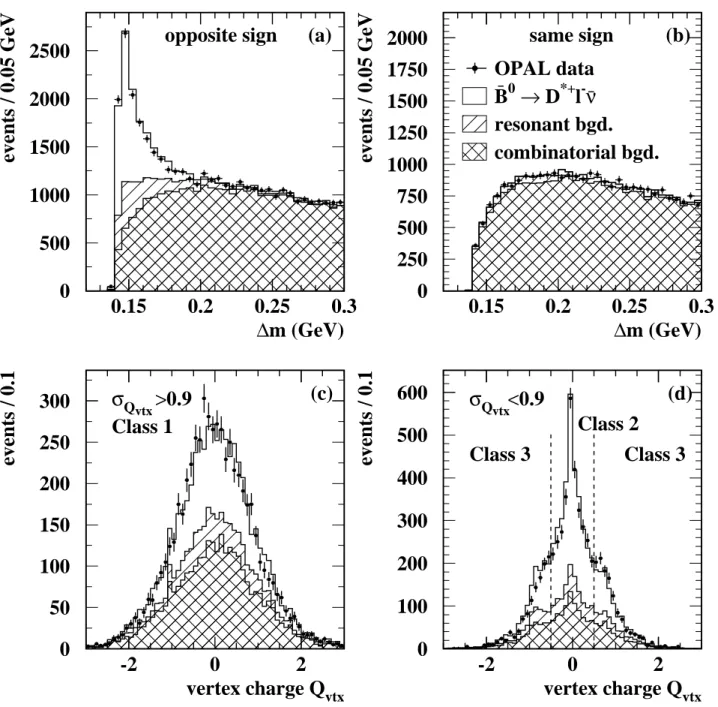
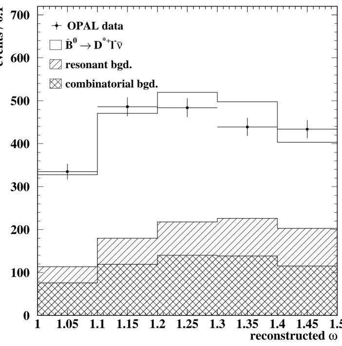
The resulting distributions of ∆mfor opposite and same sign lepton-pion combinations are shown in Figure 1(a) and (b). The predictions of the Monte Carlo simulation are also shown, broken down into contributions from signal ¯B⁰ →D^∗⁺ℓ⁻¯νevents, ‘resonant’ background containing real leptons and slow pions from D^∗⁺ decay, and combinatorial background, made up of events with fake slow pions, fake leptons or both.

In Monte Carlo simulation, about 45 % of opposite sign events with ∆m < 0.17 GeV are signal B¯⁰ →D^∗⁺ℓ⁻ν¯ events, 14 % are resonant background and 41 % are combinatorial background. The resonant background is made up mainly of B⁻ →D^∗⁺π⁻ℓ⁻ν, ¯¯ B⁰ → D^∗⁺π⁰ℓ⁻¯ν and ¯B_s →D^∗⁺K⁰ℓ⁻ν¯ decays. These are expected to be dominated by b semileptonic decays involving orbitally excited charm mesons (generically referred to as D^∗∗), e.g. B⁻ → D^∗∗⁰ℓ⁻ν¯ followed by D^∗∗⁰ → D^∗⁺π⁻. These decays will be denoted collectively by ¯B → D^∗⁺hℓ⁻ν. Small contributions are also expected¯ from b→D^∗⁺τνX decays with the¯ τ decaying leptonically, and b→D^∗⁺D⁻_s X with the D⁻_s decaying semileptonically (each about 1 % of opposite sign events). For same sign events with ∆m <0.17 GeV, there is a small resonant contribution of about 6 % from events with a real D^∗⁺ → D⁰π⁺ where the D⁰ decays semileptonically, and the rest is combinatorial background.

The most important background, from ¯B→D^∗⁺hℓ⁻ν¯ decays, comes from both charged B⁺ and neutral B⁰ and B_s decays, whereas the signal comes only from B⁰ decays. Therefore the chargeQ_vtx of the reconstructed secondary vertex containing the lepton and slow pion and its estimated errorσ_Q_vtx were calculated, using

Q_vtx = ^X

i

w_iq_i , σ_Q²_vtx = ^X

i

wi(1−wi)q_i² ,

where w_i is the weight for track i of charge q_i to come from the secondary vertex, and the sums are taken over all tracks in the jet [19,20]. The weights were calculated in a similar way to those used for the D⁰ direction reconstruction, using a neural network with the track momentum, transverse momentum and impact parameter significances with respect to the reconstructed primary and secondary vertices as inputs. The weights for the lepton and slow pion candidate tracks were set to one. The vertex charge distributions for opposite sign events with ∆m <0.17 GeV are shown in Figure 1(c) and (d).

The reconstructed vertex charge and error were used to divide the data into different classes enhanced or depleted in B⁺ decays, thus reducing the effect of this background and increasing the statistical sensitivity. Three classescwere used—class 1 where the charge is measured poorly (σQvtx >

0.9), class 2 where the charge is measured well and is compatible with a neutral vertex (σQvtx <0.9,

|Q_vtx|<0.5) and class 3 where the charge is measured well and is compatible with a charged vertex (σQvtx <0.9,|Q_vtx|>0.5).

3 Reconstruction of ω

The recoil variableωwas estimated in each event using the reconstructed four-momentum transfer to theℓ¯ν system:

q²= (E_B⁰ −E_D∗)²−(p_B⁰ −p_D∗)²

(7)

0 500 1000 1500 2000 2500

0.15 0.2 0.25 0.3 0

250 500 750 1000 1250 1500 1750 2000

0.15 0.2 0.25 0.3

0 50 100 150 200 250 300

-2 0 2 0

100 200 300 400 500 600

-2 0 2

∆m (GeV)

events / 0.05 GeV

(a) opposite sign

∆m (GeV)

events / 0.05 GeV

(b) same sign

OPAL data B⁰ → D^*+l^-ν resonant bgd.

combinatorial bgd.

vertex charge Q_vtx

events / 0.1

σ_Q >0.9 (c) Class 1^vtx

vertex charge Q_vtx

events / 0.1

σ_Q <0.9 (d) Class 3

Class 2 Class 3

vtx

Figure 1: Reconstructed ∆mdistributions for selected (a) opposite sign and (b) same sign lepton-pion combinations; reconstructed vertex charge Q_vtx distributions for opposite sign events with ∆m <

0.17 GeV and (c) σQvtx > 0.9 and (d) σQvtx < 0.9. In each case the data are shown by the points with error bars, and the Monte Carlo simulation contributions from signal ¯B⁰ →D^∗⁺ℓ⁻ν¯decays, other resonant D^∗⁺ decays and combinatorial background are shown by the open, single and cross hatched histograms respectively. The vertex charge classes 1 (poorly reconstructed), 2 (well reconstructed neutral vertex) and 3 (well reconstructed charged vertex) are indicated.

(8)

together with equation 1. The B⁰ and D^∗⁺ energies E_B⁰ and E_D^∗ were estimated directly, whilst the momentum vectors p_B⁰ and p_D∗ were estimated using the energies together with the reconstructed polar and azimuthal angles, as described in more detail below.

Since the slow pion has very little momentum in the rest frame of the decaying D^∗⁺, the momentum (and hence energy) of the D^∗⁺ was estimated by scaling the reconstructed slow pion momentum by m_D∗+/mπ, as for the D⁰ → K⁻π⁺π⁰ channel in [9]. A small correction (never exceeding 12 %) was applied, as a function of cosθ^∗, the angle of the slow pion in the rest frame of the D⁰. This procedure gave a fractional D^∗⁺ energy resolution of 15 %. The polar and azimuthal angles of the D^∗⁺ were reconstructed using weighted averages of the slow pion and D⁰ directions, giving resolutions of about 22 mrad on bothφ andθ.

The energy of the B⁰was estimated using a technique similar to that described in [21], exploiting the overall energy and momentum conservation in the event to calculate the energy of the unreconstructed neutrino. First, the energyE_bjet of the jet containing the B⁰ was inferred from the measured particles in the rest of the event, by treating the event as a two-body decay of a Z⁰ into a b jet (whose mass was approximated by the B⁰ mass) and another object making up the rest of the event. Then, the total fragmentation energy E_frag in the b jet was estimated from the measured visible energy in the b jet and the identified B⁰ decay products: E_frag=E_vis−E_ℓ−E_D∗. Finally, the B⁰ energy was calculated asE_B⁰ =E_bjet−E_frag, giving an RMS resolution of 4.4 GeV.

The b direction was estimated using a combination of two techniques. In the first, the momentum vector of the B⁰ was reconstructed from its decay products:

p_B⁰ =p_D^∗+p_ℓ+p¯ν,

the neutrino energy being estimated from the reverse of the event visible momentum vector: p¯ν =

−p_vis. The visible momentum was calculated using all the reconstructed tracks and clusters in the event, with a correction for charged particles measured both in the tracking detectors and calorimeters [17]. This direction estimate is strongly degraded if a second neutrino is present (e.g. from another semileptonic b decay in the opposite hemisphere of the event), and its error was parameterised as a function of the visible energy in the opposite hemisphere. The resulting resolution is typically between 40 and 100 mrad for bothφ and θ.

The second method of estimating the B⁰ direction used the vertex flight direction—i.e. the direction of the vector between the primary vertex and the secondary vertex reconstructed around the lepton and slow pion as described in Section 2. The accuracy of this estimate is strongly dependent on the B⁰ decay length, and was used only if the decay length significance L^′/σL^′ exceeded 3. After this cut, the angular resolution varies between about 15 and 100 mrad, and is worse for θin the 1991 and 1992 data where accuratez information from the silicon microvertex detector was not available. The B¯⁰ →D^∗⁺ℓ⁻ν¯candidate was rejected if the two reconstruction methods gaveθorφangles disagreeing by more than three standard deviations, which happened in 7 % of Monte Carlo signal events. Finally, the two B⁰ direction estimates were combined according to their estimated uncertainties, giving average resolutions of 35 mrad on φand 43 mrad on θ, including events where only the first method was used.

The estimate of q² derived from the B⁰ and D^∗⁺ energies and angles was improved by applying the constraint that the mass µof the neutrino produced in the ¯B⁰ →D^∗⁺ℓ⁻ν¯ decay should be zero.

The neutrino mass is given from the reconstructed quantities by:

µ²= (E_B⁰ −E_D^∗−Eℓ)²−(p_B⁰ −p_D^∗−pℓ)².

The constraint was implemented by calculating q² using a kinematic fit, incorporating the measured values and estimated uncertainties of the B⁰ and D^∗⁺ energies and angles (the B⁰ angular uncertainties varying event by event). This procedure improved the average q² resolution from 2.78 GeV² to 2.57 GeV². In Monte Carlo simulation, 11 % of signal events were reconstructed with q² < 0, corresponding to an unphysical value of ω larger than ω_max≈1.5, and were rejected.

(9)

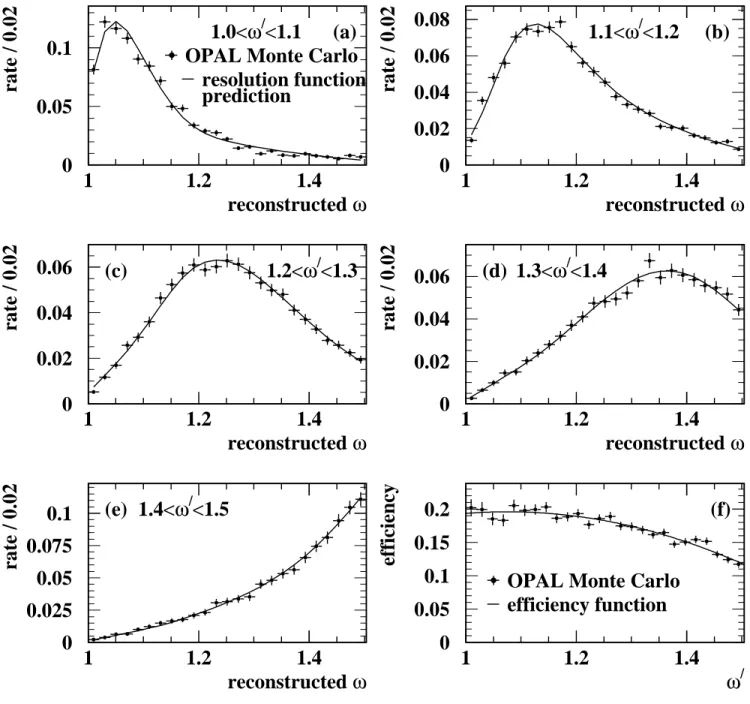
The resulting distributions of reconstructedωfor various ranges of trueω(denotedω^′) in simulated B¯⁰ →D^∗⁺ℓ⁻ν¯ decays are shown in Figure 2(a–e). The average RMS ω resolution is about 0.12, but there are significant non-Gaussian tails. The resolution was parameterised (separately for the 1991–2 and 1993–5 data) as a continuous function R(ω, ω^′) giving the expected distribution of reconstructed ω for each true value ω^′. The resolution function was implemented as the sum of two asymmetric Gaussians (i.e. with different widths either side of the peak) whose parameters were allowed to vary as a function ofω^′. The convolution of this resolution function with the Monte Carloω^′ distribution is also shown in Figure 2(a–e), demonstrating that the resolution function models the ω distributions well.

The efficiency to reconstruct ¯B⁰→D^∗⁺ℓ⁻ν¯ decays ǫ(ω^′) is shown in Figure 2(f), together with a second order polynomial parameterisation. The efficiency varies withω^′, but is reasonably flat in the critical region nearω^′ = 1 where the extrapolation to measureF(1)|V_cb|is carried out.

4 Fit and results

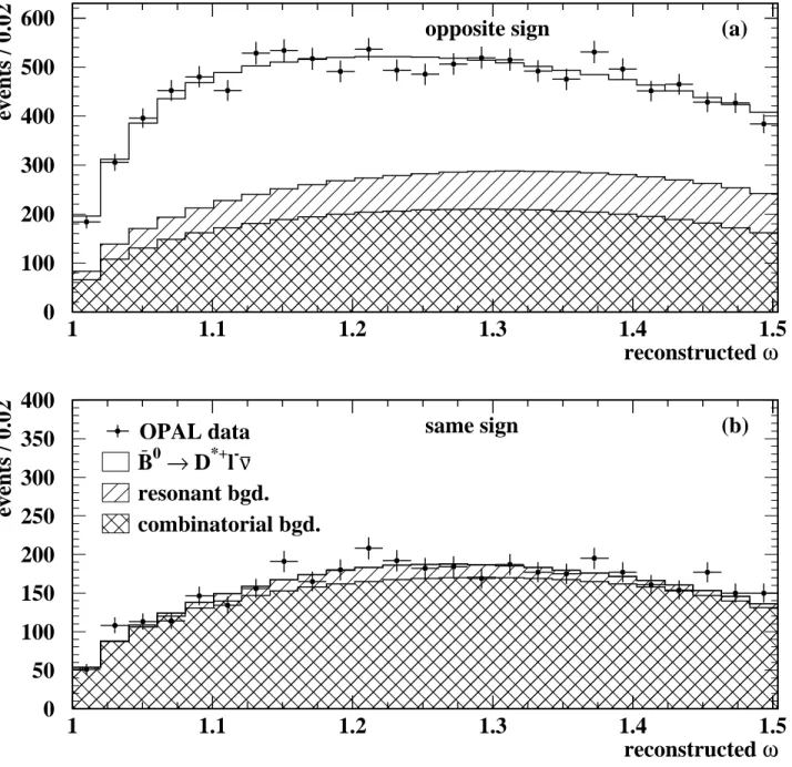
The values of F(1)|V_cb| and ρ² were extracted using an extended maximum likelihood fit to the reconstructed mass difference ∆m, recoil ωand vertex charge classcof each event. Both opposite and same sign events with ∆m <0.3 GeV andω < ωmax were used in the fit, the high ∆m and same sign events serving to constrain the combinatorial background normalisation and shapes in the opposite sign low ∆m region populated by the ¯B⁰ →D^∗⁺ℓ⁻ν¯ decays. Using the ∆m value from each event in the fit, rather than just dividing the data into low ∆m‘signal’ and high ∆m‘sideband’ mass regions, increases the statistical sensitivity as the signal purity varies considerably within the low ∆m region.

The logarithm of the overall likelihood was given by lnL=

M^a

X

i=1

lnL^a_i +

M^b

X

j=1

lnL^b_j−N^a−N^b (3)

where the sums of individual event log-likelihoods lnLâ_i and lnL^b_j are taken over all the observed Mâ opposite sign and M^b same sign events in the data sample, and Nâ and N^b are the corresponding expected numbers of events.

The likelihood for each opposite sign event was given in terms of different types or sources of event by

L^a_i(∆mi, ωi, ci) =

4

X

s=1

N_sâf_s,câ _iMs,ci(∆mi)Ps(ωi) (4) where N_sâ is the number of expected events for source s, f_s,câ is the fraction of events in source s appearing in vertex charge class c, M_s,c(∆m) is the mass difference distribution for source sin class c and Ps(ω) the recoil distribution for sources. For each source, the vertex charge fractions f_s,câ sum to one and the mass difference Ms,c(∆mi) and recoil Ps(ω) distributions are normalised to one. The total number of expected events is given by the sum of the individual contributions: Nâ=^P⁴_s=1N_sâ. There are four opposite sign sources: (1) signal ¯B⁰→D^∗⁺ℓ⁻ν¯ events, (2) ¯B→ D^∗⁺hℓ⁻ν¯ events where the D^∗⁺ is produced via an intermediate resonance (D^∗∗), (3) other opposite sign background involving a genuine lepton and a slow pion from D^∗⁺ decay and (4) combinatorial background. The sum of sources 2 and 3 are shown as ‘resonant background’ in Figure 1. A similar expression to equation 4 was used for L^b_j, the event likelihood for same sign events. In this case, only sources 3 and 4 contribute.

The mass difference distributionsM_c,s(∆m) for sources 1–3 were represented by analytic functions, whose parameters were determined using large numbers of simulated events, as were the recoil distri- butionsPs(ω) for sources 2 and 3. The fractions in each vertex charge class for sources 1–3 were also taken from simulation. For the signal (source 1), the product of the expected number of events N₁^a

(10)

0 0.05 0.1

1 1.2 1.4 0

0.02 0.04 0.06 0.08

1 1.2 1.4

0 0.02 0.04 0.06

1 1.2 1.4 0

0.02 0.04 0.06

1 1.2 1.4

0 0.025 0.05 0.075 0.1

1 1.2 1.4 0

0.05 0.1 0.15 0.2

1 1.2 1.4

reconstructed ω

rate / 0.02

OPAL Monte Carlo resolution function prediction

1.0<ω^/<1.1 (a)

rate / 0.02

1.1<ω^/<1.2 (b)

reconstructed ω

rate / 0.02

1.2<ω^/<1.3 (c)

reconstructed ω

rate / 0.02

1.3<ω^/<1.4 (d)

rate / 0.02

1.4<ω^/<1.5 (e)

ω^/

efficiency

OPAL Monte Carlo efficiency function

(f)

Figure 2: Reconstructed ω distributions for various ranges of true ω (denoted ω^′) in Monte Carlo B¯⁰ →D^∗⁺ℓ⁻ν¯events, together with the prediction from the resolution function. Events reconstructed in the unphysical region with ω > ωmax are rejected. The reconstruction efficiency as a function of true ω is also shown.