ATLAS NOTE ATLAS Public Note

(1)

ATL-PHYS-PUB-2010-009 16July2010

ATLAS NOTE

ATLAS Public Note July 15, 2010

ATLAS Sensitivity Prospects for Higgs Boson Production at the LHC Running at 7 TeV

ATLAS Collaboration

Abstract

Projections for the ATLAS sensitivity, in selected channels, to the Standard Model and Minimal Super-Symmetric Standard Model Higgs boson(s) from LHC running at 7 TeV are reported. The results are based on re-scaling expectations from detailed analyses at 10 or 14 TeV using cross-section ratios or parton distribution function re-weighting to arrive at the 7 TeV projections.

(2)

1 Introduction

The Higgs mechanism is a proposed solution to the electroweak symmetry breaking mystery which predicts the existence of an undiscovered scalar particle in the Standard Model (SM) or five such in the Minimal Supersymmetric Standard Model (MSSM). Its discovery is the primary physics goal of the Tevatron and LHC physics programs and the discovery potential has been studied extensively for the LHC running at its design energy of √s=14 TeV [1]. Combining the results from CDF and DØ, the Tevatron has recently excluded a SM Higgs boson in the mass range of 162<MH<166 GeV at 95% CL [2]. Recently, search sensitivities have been investigated for √s=10 TeV in public [3] and private documents. These new studies take into account all major backgrounds, use full simulations for both signal and background events, incorporate realistic systematic uncertainties and employ advanced statistical treatments.

At the time of writing, the LHC plan is to run at √s=7 TeV and accumulate about 1 fb⁻¹ of integrated luminosity by the end of 2011. This note assesses the reach of the ATLAS Higgs boson searches for this energy/luminosity scenario. These results are obtained by scaling the full, detailed 10 TeV (or 14 TeV) analyses [3,4] to 7 TeV using cross-section ratios at the two centre-of-mass energies, having checked that the event selection efficiencies are stable between the two energies. These results are used to to extract the approximate ATLAS sensitivity to the Higgs boson, expressed in terms of expected 95% confidence level upper limits, in selected representative channels. These are the Standard Model channelsH→WW,H→ZZ→4l andH→γγand the MSSM channelsH/A→µµ andH⁺→τν/cs.¯ This note is organised as follows. The cross-sections of the processes involved are discussed in Section 2 and systematic uncertainties are discussed in Section 3. The effects of additional minimum bias interactions per bunch crossing are addressed in Section 4. TheH→WWresults at 7 TeV are presented in Section 5. A parton distribution function re-weighting technique is also used for this channel: this is presented in Appendix A as a cross check on theH→WW cross-section scaling results. In Section 6, we describe the H→ZZ→4l results. In Section 7, we present similar results for theH→γγchannel and the statistical combination of theH →WW, H→ZZ and H→γγ is described in Section 8. We also study some MSSM channels, namely the charged Higgs search in the τν and cs¯channels (this is presented in Section 9), and theH/Adecay toµµ is described in Section 10. Finally, in Section 11, we add some concluding remarks.

2 Cross-sections

All background processes were simulated at 10 TeV and passed through the full detector simulation package [3,4]. Signal data samples were in general fully simulated, but in theH→µµchannels they have been obtained with the ATLAS fast simulation ATLFAST-II package using a parametrised description of the calorimeter response, combined with the full simulation of inner detector and muon spectrometer tracks. An excellent agreement between the ATLFAST-II and the full simulation has been demonstrated.

2.1 Background processes

In this note, for all channels studied, common values are used for the cross-sections of various background processes generated with MC@NLO [5], ALPGEN [6] or PYTHIA [7]. The resulting cross- section numbers are given in Table 1.

In addition to these there are samples of di-jet, γ-jet, Drell Yan and dedicated filtered di-leptons originating from bb, all of which were generated with PYTHIA. Further details may be found in the¯ analyses done at 10 TeV [3,4].

(3)

Process Generator Cross-section

tt¯ MC@NLO 160 pb

single top MC@NLO σs=3.9 pb,σt=58.7 pb andσWt =13.1 pb

W→lν + 0-5 partons ALPGEN/PYTHIA 31.8 nb

Z→ll+ 0-5 partons ALPGEN/PYTHIA 3.1 nb

W(→lν) +bb¯+ 0-3 partons: ALPGEN 9.5 pb

Z(→ll) +bb¯ + 0-2 partons: ALPGEN 28.9 pb

Table 1: The production cross-sections for some important background processes at 7 TeV.

2.2 Higgs Boson Productions

g g

H

(a)gg→H

q

¯ q⁰

q H

¯ q⁰

(b) VBF

q

¯ q0

H W/Z

(c)V H

g g

t¯ H t

(d)ttH¯

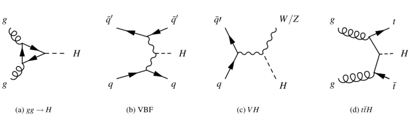
Figure 1: Representative leading order diagrams of Standard Model Higgs boson production.

At the LHC, the Higgs boson may be produced via several different processes, such as those shown in Fig. 1. These have all been calculated at NLO precision or better and the cross-sections are shown in Fig. 2. Gluon fusion, 1(a), produced through a heavy quark loop, is known at next-to-next-to-leading order (NNLO) in QCD and including electroweak (EW) corrections [8–10] with soft gluon re-summation up to next-next-to-leading log (NNLL) [11]. Vector Boson Fusion (VBF), 1(b), is known at NLO QCD and with EW corrections. The associated production with aW or aZ, 1(c), is known at NNLO QCD including EW corrections and the associated production with a pair of top quarks, 1(d), is known at NLO. In order to be consistent with the perturbative order at which the cross-section of background is calculated, the cross-sections of these processes are taken at NLO for all the SM processes considered in this paper.

The cross-sections of both signal and background processes depend strongly on √s. Cross-section ratios, defined as the cross-sections normalised to their values at √s=10 TeV, are given in Table 2 and illustrated in Fig. 3 for √svalues between 2 and 14 TeV for a few selected processes. From 10 TeV to 7 TeV, cross-section reductions are approximately 50% for the signal (MH=160 GeV), 32% forW, 40%

forWW and 60% fortt¯production.

Five Higgs bosons are predicted in the MSSM: two neutral CP-even known ashandH, one CP-odd Aand two chargedH^±. At tree level, the Higgs sector in MSSM is described by two parameters, usually chosen to be the mass of the CP-odd Higgsm_A and the ratio of vacuum expectation values tanβ. The neutral Higgs bosons are produced mainly through two processes at the LHC: in association with bottom quarks and through gluon fusion, as shown in Fig. 4.

The cross-section for the gluon fusion process is calculated in the same way as for the standard model gg H processes. The cross-section of theb-associated process can be calculated either in a

(4)

[GeV]

MH

100 150 200 250 300 350 400 450 500

H) [pb] →(ppσ

10-1

1 10 102

H (NNLO+NNLL) gg →

H (NLO) gg →

qqH (NLO) qq →

WH (NLO) q→ q ZH (NLO) q→ q

ttH (NLO) , gg → qq

7 TeV

[GeV]

MH

100 150 200 250 300 350 400 450 500

H) [pb] →(ppσ

10-1

1 10 102

H (NLO) gg →

qqH (NLO) qq →

WH (NLO) q→ ZH (NLO)q q→ q

10 TeV

[GeV]

MH

100 150 200 250 300 350 400 450 500

H) [pb] →(ppσ

10-1

1 10 102

H (NLO) gg →

qqH (NLO) qq →

WH (NLO) q→ q ZH (NLO) q→ q

14 TeV

Figure 2: Production cross-sections of the SM Higgs boson in pp collisions as functions of MH for centre-of-mass energies of 7, 10 and 14 TeV.

(5)

√s(TeV) 2 7 8 9 10 12 14

W 0.149 0.678 0.786 0.893 1.000 1.213 1.424

WW 0.061 0.597 0.728 0.863 1.000 1.273 1.568 tt¯ 0.005 0.397 0.567 0.768 1.000 1.551 2.214 gg→H 0.023 0.502 0.654 0.821 1.000 1.393 1.825 qq→qqH 0.019 0.502 0.657 0.830 1.000 1.405 1.856

Table 2: Relative NLO cross-sections from MCFM [12] at different ppcollision energies for the signal and main background processes. The Higgs boson mass is taken as 160 GeV for the signalgg→Hand qq→qqH processes.

(TeV)

2 4 6 8 10 12

s

14

Relative Cross Section

0 0.5 1 1.5

2 2.5

W WW

tt →H (160 GeV) gg

qqH (160 GeV)

→ qq

Figure 3: Relative NLO cross-sections from MCFM [12] as functions of √s for the signal (MH = 160 GeV) and main background processes.

4-flavor scheme asgg→bbH¯ or in a 5-flavor scheme asbb¯→H, where the difference in the number of flavors refers to whether or notb-quarks are included as an active flavor in the parton density functions of protons. Higher order QCD corrections have been calculated up to NLO for the 4-flavor scheme [13, 14] and NNLO for the 5-flavor scheme [15]. The charged Higgs bosons can be directly produced in association with top quarks, but this note only considers production indirectly from top quark decays (t →H⁺b), i.e.,M_H^± <mt. Partial NNLO corrections are available for thett¯process [16], the dominant top quark source fort→H⁺bdecays. The branching ratio oft→H⁺bis evaluated with FeynHiggs [17–

20]. Heavy charged Higgs cross-sections are estimated at NLO [21]. Apart from QCD corrections at NLO or higher, all calculations also contain the leading supersymmetric corrections, the so-called ∆mb

corrections [21], leading to a reduction factor

f = (1+∆mb)⁻². (1)

The heavy H⁺ cross-sections with QCD corrections at NLO have to be multiplied with this factor to include the leading supersymmetric corrections. The value of∆m_bcan be calculated with FeynHiggs for MSSM scenarios defined at the weak scale.

Along with the improvement of theoretical calculations, recent advances in constraining parton density functions (PDF) have also contributed significantly to our improved knowledge of the Higgs boson production cross-sections. Most of these calculations use MSTW2008 (LO, NLO, NNLO) and CTEQ6.6 (NLO) [22] PDF sets.

(6)

Figure 4: Tree-level Feynman diagrams for the neutral MSSM Higgs boson production via (a) gluon fusion and (b) the associated production withb-quarks.

The production cross-sections and decay branching ratios of the Higgs bosons depend on a large number of standard model parameters. Unless otherwise specified, the followingdefaultparameter sets are used: m_uds=190 MeV, m_c =1.40 GeV, m_b=4.75 GeV, m_t =172.5 GeV, M_W =80.398 GeV, MZ=91.1876 GeV andGF =1.16639×10⁻⁵ GeV⁻². Pole quark mass values are quoted here. The strong coupling constant αs is in general taken to be the value from the PDF set used. MSTW2008 determines the αsvalue as part of its PDF fit: αs(M_Z) =0.13939 at LO, 0.12018 at NLO and 0.11707 at NNLO. On the other hand, the CTEQ collaboration uses the world average values (αs(MZ) =0.130 at LO andαs(MZ) =0.118 at NLO) for its PDF fits.

The cross-section changes with the renormalisation scale µR and factorisation scales µF as a result of uncalculated higher order effects. Starting from a median scale µ0, which is considered the “natural scale” of the process and is expected to absorb the large logarithmic corrections, the current standard convention is to vary the two scales, either collectively or independently, within µ0/ξ ≤µR,µF ≤ξ µ0. Depending on the process,ξ =2 or larger. The variation of the scales results in a uncertainty band: the narrower the band is, the smaller the higher-order corrections are expected to be. This is by no means a rigorous way to estimate the theoretical uncertainty.

2.3 Higgs Boson Decays

The SM Higgs boson decay branching ratios have been estimated taking into account several contributions, namely those included in HDECAY [23] and PROPHECY4f [24] with the addition of the full two-loop EW corrections evaluated in [25].

The HDECAY program calculates the decay widths and branching ratio of the Higgs boson(s) in the SM and in the MSSM. For the SM specifically, it includes all the channels kinematically allowed (also the loop mediated ones), all the relevant higher order QCD corrections to the decays into quark pairs and into gluons (quark loop mediated decays) and the double off-shell decays of the Higgs boson into massive gauge bosons which then decay into four massless fermions.

PROPHECY4f is a Monte Carlo event generator for the specific simulations of the Higgs boson decay H→ZZ/WW → 4 fermions (leptonic, semi-leptonic and four-quark) final states. The calculation of the complete electroweakO(α)and QCDO(αs)corrections to the processesH→4f, includes both the corrections toWW andZZdecays and their interference. The QCD corrections additionally include leading 2-loop corrections from the Higgs boson self-interaction as discussed in [26]. The intermediate gauge bosons are treated as resonances (and their widths calculated at NLO), without any on-shell approximation and the calculation covers the full Higgs boson mass range near, and below the gauge-boson pair thresholds. The bottom quark is treated like any other massless quark. PROPHECY4f provides Γ(LO) and Γ(NLO) partial width to any of the possible 4f final states. The H→WW/ZZ on-shell

(7)

processes give the width for the decay into a pair of on-shell massive gauge bosons at leading and next- to-leading order. The Higgs-boson-mass-enhanced two-loop terms have also been included in the NLO result. The decays of theW/Z bosons are not included here. Using the LO/NLOW/Z widths in the LO/NLO calculation ensures that theeffectivebranching ratios of theW/Zobtained by summing over all decay channels add up to one.

References [25, 27–30] evaluate the corrections to theH→γγ decay. The EW corrections are numerically small and have opposite sign with respect to the NLO QCD correction, resulting in a partial cancellation of the two effects. Recently, the results in [25, 27–30] have been updated to include the accurate description of the effects in proximity of the threshold forWW andZZ production, removing the spikes present in [25] and extending the validity of [29] tillMH<mt+MW.

Under the assumption that EW corrections factorise with respect to the QCD dynamics, they result in a factor 1+δ_γγ^EWmultiplying the QCD results (for fixedMH). The exact validity of this approximation has been discussed in [31]. The authors evaluate numerically the sub-leading EW×QCD (3-loop) mixed terms which appear in the exact calculation under the assumption that the large logarithms due to the soft and collinear initial state radiation factorise, and found them to be small and not factorising. Therefore, excluding unexpected discoveries (e.g. if the large soft and collinear logarithms were not to factorise with respect to the NLO EW corrections), the assumption of factorisation between EW and QCD dynamics represents a good approximation of the higher order corrections to Higgs boson cross-section and decay.

In this approximation, the partial width ofH→γγ, can be written as

Γ_γγ(MH) = [1+δ_γγÊW(MH)]·[1+δ_γγ^QCD(MH)]·Γ⁰_γγ (2) HereΓ⁰_γγ is the partial decay width at the leading order, δ_γγÊW andδγγ^QCD are higher order EW and QCD corrections. δ_γγÊWvalues have been calculated in [25]. The HDECAY program calculates[1+δγγ^QCD]Γ⁰_γγ as a whole. As mentioned, δ_γγÊWand δγγ^QCD tend to cancel to a large extent. The correction factor δ_γγÊW contains:

• The exact dependence on the light quark corrections as in [25] improved by the use of complex masses forW andZ;

• The effect of heavy quark corrections as described in [30] forMH<150 GeV.

The state of the art prediction for the Higgs boson width includes the results from HDECAY, plus the EW NLO corrections described above, plus the fullH→4 fermions from PROPHECY4f. Operatively, the Higgs boson total decay width given by HDECAY has been modified according to the following prescription:

ΓH=Γ^HD−Γ^HD_ZZ −Γ_WW^HD +Γ^PR₄_f +Γ^HD_γγ ·

δ_γγ^EW+δ_γ^QED_e+e⁻

, (3)

where Γ_H is the total Higgs boson width, Γ^HD is the Higgs boson width reported by HDECAY, and Γ^HD_ZZ and Γ_WW^HD stand for the partial Higgs boson width to ZZ andWW calculated with HDECAY, respectively, while Γ^PR_4f represents the partial width of H →4f calculated with PROPHECY4f. The additionalΓ^HD_γγ andδ_γγ^EWterms represent the partial width ofH→γγ calculated with HDECAY and the EW corrections to this decay. Finally, δ_γ^QED_e+e⁻ corresponds to the fractional contribution of the partial width ofH→γe⁺e⁻with respect toΓ^HD_γγ [32].

The branching ratios of the MSSM Higgs bosons are evaluated using FeynHiggs [19,20].

3 Statistical and Systematic Uncertainties

The analyses in this note present expected 95% CL upper limits on various Higgs cross-sections. These are based on the observed number of signal candidate events and the expected number of background

(8)

events in the signal region. In some cases the results are extracted using a fit in the region of inter- est. In addition to statistical uncertainty there are theoretical and experimental systematic uncertainties which affect the result. Unless otherwise specified, the limit setting procedure uses the profile likelihood method [1] that can be described as follows: given a Likelihood function, a Likelihood Ratioλ(µ) (where µ a is a signal normalisation parameter) is computed by maximising the Likelihood function twice, once on its full set of free parameters, and once with µ restricted to a particular value. (In the fit where µ is allowed to float, it is forced to be positive.) The Likelihood Ratio is then defined as λ(µ) =L(µ,θˆˆ)/L(µˆ,θˆ), where ˆµ is the preferred value of µ in the first fit, ˆθ represents the set of the preferred values of all nuisance parameters in the first fit, and ˆˆθ represents the preferred values of all nuisance parameters in the second fit. Forµ >0, the estimatorqµ is defined to be−2lnλ(µ)ifµ <µˆ or zero otherwise; forµ =0 it is simply−2lnλ(µ)sinceµis required to be nonnegative. In the limit of large numbers of events and large sensitivity, this estimator is distributed as a “half-χ²” distribution [1]

whenµ coincides with the true value ofµ and a non-central χ²distribution otherwise. Given a hypothesised value of µ, the asymptotic form of the µ =µtrue distribution can be used to estimate a p-value by integrating the asymptotic distribution from the observed value ofq_µ to infinity. The upper bound on the signal production cross-section is obtained by finding the largest value ofµ for which the p-value is larger than a specified threshold, in this case 0.05. In practice, finding this value entails scanning over hypothesised values ofµ. The upper bound is the point where the p-value for the correspondingq_µ is 0.05.

The major detector-related contributions to the systematic uncertainties come from the uncertainties in the lepton, photon, jet and missing energy reconstruction and identification efficiencies, the momentum or energy resolution, and the momentum or energy scale of the reconstructed objects. The magnitudes of these uncertainties are summarised in [1]. The uncertainty on the luminosity for the early data period of 2010-2011 is taken to be 10% in the studies discussed herein.

Theoretical uncertainties are also taken into account in the analyses reported in this paper. The major theoretical uncertainties in the prediction of the background cross-sections are the PDF uncertainties and uncertainties related to the QCD renormalisation and factorisation scales. These scale uncertainties reflect the uncertainty on the estimated cross-section owing to the omission of higher order terms in the perturbative expansion of the process.

Additional systematic uncertainties relevant to the individual channels are discussed in the appropri- ate sections below.

4 Effect of pile-up and Cavern Background

Additional minimum bias interactions may occur on top of the event that triggers the detector readout:

this is referred to as pile-up. In addition, neutrons may fly in the ATLAS cavern for a few seconds until they are thermalised, thus producing a kind of a permanent neutron-photon gas which creates a constant rate of Compton electrons and spallation protons. This component, i.e. additional hits created by long- lived particles, is referred to as cavern background. The effects of both pile-up and cavern background in the analysis have been studied in the three different luminosity scenarios which are summarised in Table 3. In the scenario C mentioned in Table 3, pile-up effects lead to a 10% decrease of the VBF H→ WW →lνlν signal survival probability due to a less efficient central jet veto. Some of the background rates, such astt¯production, remain unaffected by the additional minimum bias interactions. However, in some cases, such asZ(→ll) +X, the background rates increase (with respect to the no-pile-up case) due to increased jet activity from additional minimum bias events. A careful optimisation of the cuts and the usage of the anti-Kt [33] based jet algorithm, which is more robust against pile-up than the cone algorithm used in [1], will keep these backgrounds under control.

(9)

Scenario Luminosity (cm⁻²s⁻¹) Bunch Crossing Time (ns) Events/Bunch Crossing

A 1· 10³³ 75 6.9

B 2· 10³³ 25 4.6

C 1· 10³² 450 4.1

Table 3: The luminosity scenarios used to quantify the effect of the pile-up and cavern background.

Relative Luminosity Scenario

Efficiency A B C

H→4µ -5.2% -6.0% -3.0%

Table 4: Relative change of theH→ZZ→4µ signal selection efficiency due to the influence of pile-up and cavern background, shown after all analysis cuts for the three luminosity scenarios discussed in Table 3. The effect is smaller for scenario A than for scenario B because of the smaller cavern background event rate normalisation used for scenario A compared to scenario B.

TheH→ZZ→4µ (mH=130 GeV) signal selection efficiency as a function of the selection cuts is shown in Fig. 5 for luminosity scenario B (see Section 6.2 for details on the selection cuts). In this figure, the approach to the track isolation requirement used in the reference analysis at√s=14 TeV is compared with the new approach that rejects tracks originating from pile-up vertices by requiring their longitudinal impact parameter with respect to the primary vertex to be less than 10 mm, with a pT cut of 1 GeV on the track transverse momentum. The latter method, which is currently the default, cancels almost fully the influence of pile-up on the track isolation. The remaining decrease of the selection efficiency with respect to the case without pile-up and cavern background is mainly due to the calorimeter isolation requirement, which can be partly recovered by re-adjusting the actual cut value. The effect of pile-up on the signal selection efficiency is reported in Table 4; in the worst case it amounts to a relative reduction by about 6% with respect to the case without pile-up and cavern background.

Pile-up effects are also considered for the light charged Higgs studies using scenario C of Table 3, especially for theH⁺→cs¯channel. It was observed that the event counts after each cut remain consistent with those obtained without pile-up, within statistical uncertainties, i.e., pile-up does not significantly affect the results. The same conclusion was drawn in the study of the SM di-lepton tt¯cross-section measurement in ATLAS [34].

The pile-up and cavern background expected for early running conditions leading up to the accu- mulated integrated luminosity of 1 fb⁻¹at 7 TeV centre-of-mass energy would be less than reported in Table 3 so that additional minimum bias interactions and cavern background in the early data will not change the conclusions of the analyses reported herein.

5 H → WW → lν lν

We present two methods for the extrapolation of the 10 TeVH→WW results [3] to 7 TeV: by scaling according to the cross-section ratios or by PDF re-weighting. The cross-section scaling is motivated by earlier studies that showed that the signal gg→H and the Standard ModelWW efficiencies are effectively constant for √s_∼^>6 TeV. The PDF re-weighting method, which is used here as a cross check of the cross-section scaling, is described in detail in Appendix A. The results are very similar.

(10)

Selection Step

Preselection

Z1

M

Z2

M Track Isol. Calo Isol. IP Sign.

MH

Signal Efficiency

0.25 0.30 0.35 0.40 0.45 0.50 0.55 0.60 0.65 0.70

No Pile-Up

>1 GeV Pile-Up / Si Hits + PT

<10 mm Pile-Up / Si Hits + z0

ATLAS Preliminary (Simulation)

µ 4

(*)→ ZZ

→ H

Figure 5: H→ZZ→4µ signal selection efficiency as a function of the selection step for the luminosity scenario B, as defined in Table 3. The open boxes correspond to the case without pile-up and cavern background. The dark solid circles correspond to the sample with pile-up and cavern background, with a track isolation requirement along the lines of the reference analysis at √s=14 TeV. The pale circles correspond to the pile-up case with the improved track isolation requirement.

5.1 Systematic Uncertainties onH→WW

In the H→WW analysis, background contributions were estimated from control regions [3] with extrapolation parameters (α and β) that are taken from Monte Carlo. Theα parameter of a background process is defined to be the ratio of its contributions to the signal and control regions, whileβis a parameter to correct for contamination in the control region from other background processes [3]. Systematic uncertainties on these parameters, listed in Table 5 forH→WW, are quite large; many of them are con- sequences of low Monte Carlo statistics. These large systematic uncertainties often lead to diminishing returns for increasing integrated luminosity but it is reasonable to expect significant reductions in these systematic uncertainties as the size of the data sample increases. For the study of theWW channel below, we consider two scenarios of the systematic uncertainties on these extrapolation parameters: (1) taking the systematic uncertainties from the 10 TeV study as listed in Table 5, which we call the conservative scenario; (2) capping the systematic uncertainties on the extrapolation parameters α and β for the top andW+jets backgrounds at 10%, referred to as the optimistic scenario. The choice of 10% is no doubt aggressive. It will require high quality data, well understood detector performance and minimisation of theoretical uncertainties. Though the uncertainties discussed here are onα’s andβ’s, it should be noted that systematic uncertainties on background estimations are given by the uncertainties onα’s for almost all cases.

Analysis channel σαWW σαtop σαW+jets σ_β_top σ_β_W+jets

H+0j 7.3% 108% 100% 74% 100%

H+1j 17% 52% 91% 20% 78%

H+2j 54% 43% − 18% −

Table 5: Relative systematic uncertainties on the extrapolation parameters that are used to estimate background contributions from control regions in theH→WW analysis at 10 TeV [3].

In theH→WW analysis, uncertainties on theoretical cross-sections are not included in the system-

(11)

atic uncertainties [3]. For background estimations, this is justified by using the control region for real data analysis. What matters is the relative contributions (α’s andβ’s) to the signal and control regions from a background process. The SM signal cross-sections are taken at NLO in this analysis as explained in Section 2.2 although NNLO+NNLL corrections are available. The systematic uncertainties in the NLO cross-sections will tend to reduce the projected sensitivity. However, this will be compensated by the increase in the cross-sections coming from the NNLO+NNLL corrections.

5.2 Expected cross-section limits onH→WW

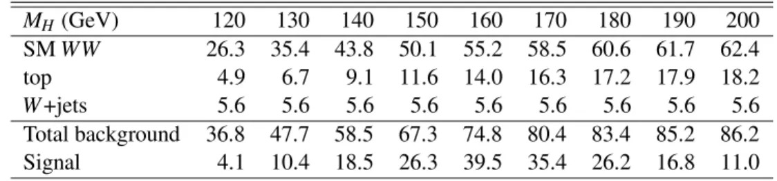
The estimated numbers of events in 1 fb⁻¹of data are shown in Table 6.

M_H(GeV) 120 130 140 150 160 170 180 190 200

SMWW 26.3 35.4 43.8 50.1 55.2 58.5 60.6 61.7 62.4

top 4.9 6.7 9.1 11.6 14.0 16.3 17.2 17.9 18.2

W+jets 5.6 5.6 5.6 5.6 5.6 5.6 5.6 5.6 5.6

Total background 36.8 47.7 58.5 67.3 74.8 80.4 83.4 85.2 86.2

Signal 4.1 10.4 18.5 26.3 39.5 35.4 26.2 16.8 11.0

Table 6: Estimated number of events for the signal and the major backgrounds at an integrated luminosity of 1 fb⁻¹for√s=7 TeV after the full event selection inH→WW →lνlν.

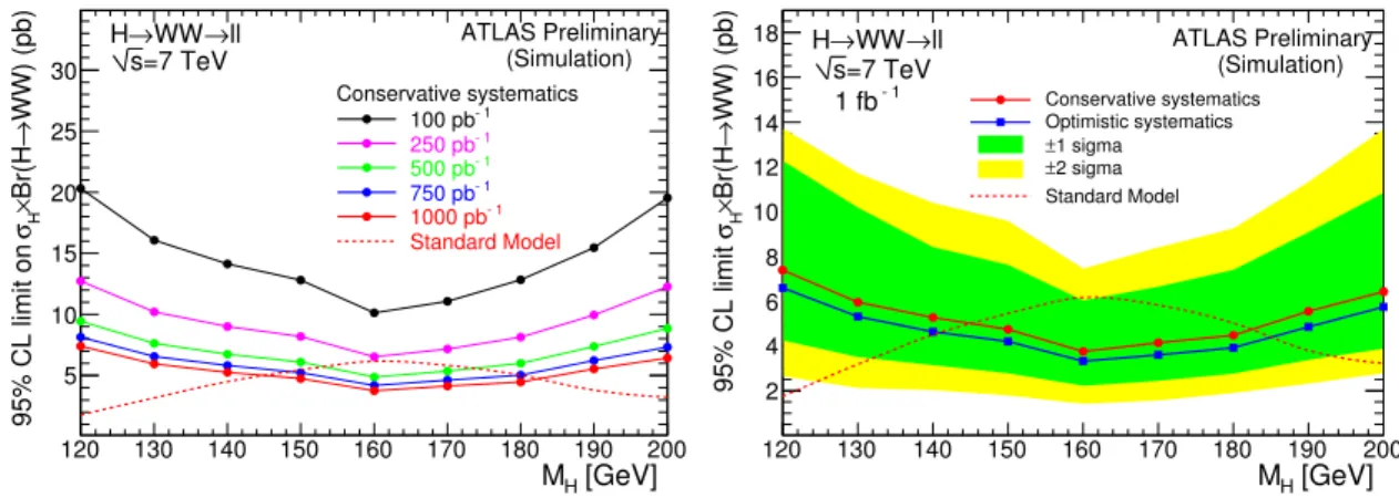
The expected 95% CL upper limits on the productσH×B(H→WW)of the Higgs boson production cross-section and its decay branching ratio are given in Table 7 for 1 fb⁻¹ of integrated luminosity at 7 TeV. The left plot of Fig. 6 shows the expected 95% CL upper limits on σH×B(H →WW) for different integrated luminosity scenarios at √s=7 TeV assuming the conservative systematics. The right plot of Fig. 6 shows the expected 95% CL upper bounds onσH×B(H→WW)(with uncertainty bands corresponding to one and two standard deviations) for the two systematic assumptions, for 1 fb⁻¹ at 7 TeV.

M_H(GeV) 120 130 140 150 160 170 180 190 200

SMσH×B(H→WW) 1.76 3.18 4.50 5.45 6.17 5.83 5.03 3.80 3.23 Conservative systematics 7.4 5.9 5.3 4.7 3.8 4.1 4.5 5.5 6.4 Optimistic systematics 6.6 5.3 4.6 4.2 3.3 3.6 3.9 4.9 5.7 Table 7: The standard model cross section ofσH×B(H→WW)in pb and the expected upper limits at 95% CL for 1 fb⁻¹ at√s=7 TeV and the two systematic uncertainty assumptions. The limits are computed assuming only backgrounds are present.

5.3 Interpretation of the cross-section limits onH→WW

The expected 95% CL upper limits on the Higgs boson production cross-section normalised to the Stan- dard Model expectation for different integrated luminosity scenarios at √s =7 TeV and for the two background systematic uncertainty assumptions are tabulated in Table 8 and illustrated in Fig. 7.

The expected 95% CL upper limits on the Higgs boson production cross-section normalised to the Standard Model expectation are tabulated in Table 8 for 1 f b⁻¹of integrated luminosity at 7 TeV. The left plot of Fig. 7 shows the expected 95% CL upper limits of the Higgs production cross-section normalised to the SM expectation for different integrated luminosity scenarios at √s=7 TeV assuming the conservative systematics. The right plot of Fig. 7 shows the expected 95% CL upper bounds on the Higgs

(12)

[GeV]

MH

120 130 140 150 160 170 180 190 200 WW) (pb)→Br(H×Hσ95% CL limit on

5 10 15 20 25 30

100 pb-1

250 pb-1

500 pb-1

750 pb-1

1000 pb-1

Standard Model Conservative systematics ll

WW→ H→

=7 TeV

s ATLAS Preliminary

(Simulation)

[GeV]

MH

120 130 140 150 160 170 180 190 200

WW) (pb)→Br(H×Hσ95% CL limit ₂

4 6 8 10 12 14 16 18

Standard Model Conservative systematics Optimistic systematics

1 sigma

±2 sigma

±

ll WW→ H→

=7 TeV s -1

1 fb

Figure 6: Expected 95% CL upper limits onσH×B(H→WW)in pb. The left plot shows the conservative systematic uncertainty assumptions for different integrated luminosity scenarios. The right plot has green and yellow bands representing the range in which we expect the limit will lie, depending upon the data and lines showing conservative and optimistic uncertainty scenarios. The Standard Model cross-section is shown a red dotted line.

production cross-section normalised to the SM expectation (with uncertainty bands corresponding to one and two standard deviations) for the two systematic assumptions, for 1 fb⁻¹at 7 TeV.

MH(GeV) 120 130 140 150 160 170 180 190 200

Conservative systematics 4.2 1.9 1.2 0.87 0.61 0.71 0.89 1.5 2.0 Optimistic systematics 3.8 1.7 1.0 0.77 0.54 0.62 0.78 1.3 1.8

Table 8: Expected upper limits at 95% CL of the Higgs boson production cross-section normalised to the cross-section predicted by the Standard Model for 1 fb⁻¹ at √s=7 TeV and the two systematic uncertainty assumptions used the inH→WW→lνlν analysis.

For the mass region where the expected upper limit on the normalised cross-section is less than one, the probability to exclude the Standard Model Higgs boson if it does not exist is at least 50%. In the most favourable case ofM_H=160 GeV, a minimum of∼250 pb⁻¹is required to be sensitive to the SM Higgs boson. The differences between the two background uncertainty scenarios are small, particularly for low integrated luminosities. This is attributed to the dominance of the statistical uncertainties at low luminosities. The limits for 1 fb⁻¹are also shown in Fig. 7, along with their variations corresponding to one and two standard deviations.

For an integrated luminosity of 1 fb⁻¹ of high quality and well understood data, it is possible to exclude the SM Higgs boson in the mass range of 140−185 GeV at 95% CL for the optimistic systematic scenario. The potential exclusion mass range for the conservative scenario is slightly smaller. The minimum integrated luminosities for expected exclusion and discovery are listed in Table 9, where a discovery is defined as an observation of 5σ significance.

6 H → ZZ → 4l

Experimentally, the cleanest signature for the search of the Higgs boson is its “golden” decay into four leptons: H→ZZ⁽^∗⁾→4l, wherel=e,µ. An excellent energy and momentum resolution for the reconstructed electrons and muons, respectively, leads to a narrow four-lepton invariant mass peak on top of a smooth background. The major component of the background is the irreducible ZZ⁽^∗⁾→4l process.

(13)

[GeV]

MH

120 130 140 150 160 170 180 190 200

95% CL Limit / SM

1 10

100 pb-1_-1

250 pb 500 pb-1_-1

750 pb 1000 pb-1

Conservative systematics ll

WW→ H→

=7 TeV

s ATLAS Preliminary

(Simulation)

[GeV]

MH

120 130 140 150 160 170 180 190 200

95% CL Limit / SM

1

10 Conservative systematics

Optimistic systematics 1 sigma

± 2 sigma

±

ll WW→ H→

=7 TeV s1 fb -1

Figure 7: Expected 95% CL upper limits of the Higgs boson production cross-section normalised to the cross-section predicted by the Standard Model. Left: for different integrated luminosity scenarios at

√s=7 TeV and conservative systematic uncertainty assumptions. Right: the green and yellow bands represent the range in which we expect the limit will lie, depending upon the data, normalised to the SM cross-section for an integrated luminosity of 1 fb⁻¹. The effect of conservative and optimistic systematic uncertainties is indicated.

MH(GeV) 120 130 140 150 160 170 180 190 200

Conservative Exclusion 210 12 1.6 0.68 0.28 0.41 0.76 2.7 4.5 Optimistic Exclusion 50 4.5 1.1 0.54 0.25 0.33 0.58 1.8 3.4

Conservative Discovery 1100 95 18 16 4.8 6.6 17 68 96

Optimistic Discovery 230 36 8.1 5.5 2.3 3.1 6.7 31 52

Table 9: Minimum integrated luminosities in fb⁻¹required at√s=7 TeV for a 95% CL exclusion and 5σ discovery for the two systematic uncertainty assumptions in the H→WW channel.

In the high mass region –MH>180 GeV – the signal signature is characterised by the two on-shell Z bosons decaying into lepton pairs, which strongly suppress any reducible background contributions. In the low Higgs mass region –MH<180 GeV – where one of the Z bosons is off-shell, thus decaying into low transverse momentum leptons, the reducible backgrounds fromZ+jets andtt¯are important in addition to the irreducible background and require tight lepton isolation cuts to keep their contribution well below theZZ⁽^∗⁾continuum. The most challenging mass region is around 160 GeV, where the branching ratio for H→ZZ^∗ decays is suppressed owing to the opening of the phase space for the Higgs boson decay into two on-shellW bosons.

6.1 Signal and Backgrounds toH →ZZ

The Higgs production cross-sections at√s=7 TeV are summarised in Table 10. The expected yields of signal and background events at√s=7 TeV are summarised in Table 11.

MH(GeV) 120 140 150 170 180 190 200 240 300 400 500 600

σNLO·B[fb] 0.90 2.92 3.06 .65 1.43 4.41 4.82 3.82 2.68 1.85 0.79 0.35

Table 10: NLO Higgs to four lepton production cross-sections at √s=7 TeV, including the branching ratioH→ZZ⁽^∗⁾and the subsequent decayZ→ll(l=e,µ).

(14)

MH(GeV) 120 130 140 150 165 170 180 190 SM ZZ 0.090 0.094 0.083 0.089 0.121 0.147 0.376 0.981 top & Z+jets 0.005 0.004 0.005 0.004 0.005 0.005 0.003 0.003 Total background 0.095 0.098 0.088 0.093 0.126 0.152 0.379 0.984 Signal 0.105 0.319 0.595 0.713 0.185 0.192 0.458 1.49

MH(GeV) 200 220 240 260 300 400 500 600

SM ZZ 1.29 1.18 0.92 0.89 0.72 0.48 0.49 0.39

Signal 1.60 1.46 1.25 1.08 0.88 0.67 0.29 0.13

Table 11: Estimated number of events in the signal region for the signal and the major backgrounds at an integrated luminosity of 1 fb⁻¹for√s=7 TeV after the full event selection inH→ZZ→4l(the 4e, 2e2µ and the 4µ final states are summed) .

6.2 Signal and background efficiencies between√s=10TeV and√s=7TeV forH→ZZ The estimation of the expected signal and background rates at √s=7 TeV using cross-section scaling of the √s=10 TeV result incorporates the implicit assumption of constant event selection efficiency for the two different centre-of-mass energies. In order to test this assumption, we have used example reference signal and background samples simulated for √s=7 TeV, and compared the most relevant distributions and event selection efficiencies to the corresponding 10 TeV data. Three signal samples with Higgs masses of 130, 150 and 300 GeV and the irreducible ZZ background sample were used.

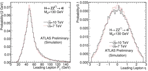
In Fig. 8, the pT and η distributions of the leading lepton originating from the Higgs decay are compared, respectively, for√s=7 TeV and√s=10 TeV. It is noted that the differences in thepTdistri- butions are marginal, while for the lower centre-of-mass energy the leptons tend to be in the more central region of the detector, with lower pseudo-rapidity. The kinematic similarity of the final state in both centre-of-mass energies indicates that the signal selection efficiency will not vary substantially. Further- more, it is expected that for √s=7 TeV the selection efficiency will be slightly higher with respect to the corresponding efficiency at√s=10 TeV, owing to the higher centrality of the leptons.

(GeV) Leading Lepton PT

0 20 40 60 80 100 120 140

Probability/(2 GeV)

0.00 0.01 0.02 0.03 0.04 0.05 0.06

0.07 HH→→ ZZ ZZ^(*)^(*)→→ 4l 4l

=130 GeV MH

=10 TeV s=7 TeV s

Leading Lepton η

-3 -2 -1 0 1 2 3

Probability/0.1

0.000 0.005 0.010 0.015 0.020 0.025 0.030 0.035

→ 4l ZZ(*)

H→

=130 GeV MH

=10 TeV s=7 TeV ATLAS Preliminarys

(Simulation)

Figure 8: Comparison of the lepton pT and η distributions fromH →ZZ⁽^∗⁾→4l decays, withMH= 130 GeV, at√s=10 TeV and√s=7 TeV. Similar agreement is observed for the sub-leading leptons.

(15)

ForMH<220 GeV, the mass resolution of the Higgs candidates directly affects the sensitivity of the Higgs searches. However, the leading di-lepton corresponds to an on-shellZ boson. Thus an improvement in the Higgs mass resolution can be achieved by applying theZ mass constraint to the lepton pair with mass closest to theZ mass. ForMH >220 GeV, where bothZ bosons are on-shell, theMZ constraint is applied to both lepton pairs. However, for Higgs masses>220 GeV the Higgs natural width dominates over the detector resolution and as a result the improvement in the Higgs mass resolution is less important for the discovery potential. One additional advantage offered by theZmass constraint is the reduced sensitivity of the obtained resolution to mis-calibrations and mis-alignments of the detector.

In Fig. 9, the maximum impact parameter significance distributions are shown for the signal and theZbb¯ background in the left plot, and the mass resolution is shown as a function of the Higgs mass in right plot, for theH→4µ channel. The maximum impact parameter significance is one of the discriminating variables considered in the analysis.

d0

/σ Maximum d0

0 2 4 6 8 10 12 14

Probability/0.5

10-3

10-2

10-1 H(130 GeV)→ ZZ^(*)→ 4µ b

Zb

(GeV) MH

100 200 300 400 500 600

Resolution (GeV)

0 2 4 6 8 10 12

µ 4

(*)→ ZZ

→

H No M_Z Constraint Constraint With MZ

Figure 9: Left plot: distributions of the maximum impact parameter significance for the signal and the Zbb¯ background in theH→4µ channel. Right plot: invariant mass resolution for theH→4µ channel as function of the Higgs mass, before and after applying theZmass constraint.

Performing the H →4l analysis on selected signal samples at √s=7 TeV, namely MH =130, 150 and 300 GeV, and on the irreducible ZZ background, demonstrated that the selection efficiencies obtained for the two different centre-of-mass energies agree to within 2%. Based on this result, and the kinematic distributions of signal and background in the two centre-of-mass energies, it is concluded that the assumption of constant signal and background efficiencies is a reasonable approximation in order to obtain a sensitivity estimate at√s=7 TeV by scaling the results extracted at√s=10 TeV.

6.3 Expected Exclusion Limit onH→ZZ

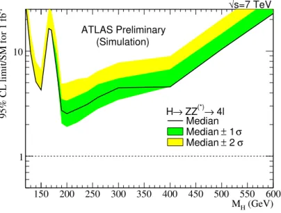
The expected exclusion limits on the Standard Model production cross-section times branching ratio in the decay channelH→ZZ⁽^∗⁾→4lare presented in Fig. 10 as a function of the Higgs boson mass. The results are presented in terms of the expected exclusion limit on the cross-section times branching ratio, divided by the corresponding Standard Model prediction. If the result is less than one at some mass, then the probability of correctly excluding a non-existent SM Higgs is at least 50%.

The limit shown in Fig. 10 is strictly valid only for the Standard Model. For large Higgs boson masses, the natural width predicted by the Standard Model is larger than the experimental resolution, and a truly model-independent treatment would take into account the fact that other models might have a Higgs boson with a natural width different from the Standard Model value.

With an integrated luminosity of 1 fb⁻¹at 7 TeV the Standard Model Higgs boson cannot be excluded at the quoted confidence level for any mass value in theH ZZ 4l channel alone. The analysis is

(16)

(GeV) MH

150 200 250 300 350 400 450 500 550 600

-1 95% CL limit/SM for 1 fb

1 10

→ 4l ZZ(*)

H→

Median 1 σ Median ±

σ 2

± Median

s=7 TeV

√ ATLAS Preliminary

(Simulation)

Figure 10: Expected 95% CL upper limits on the Standard Model Higgs boson production in theH→ ZZ⁽^∗⁾→4l channel as a function of the Higgs mass, for the 7 TeV centre-of-mass energy. The bands indicate the range in which we expect the limit will lie, depending upon the data. These limits were obtained with theCLSmethod used in LEP and Tevatron experiments [35].

most sensitive for a Standard Model Higgs mass of about 200 GeV where an upper bound in the cross- section times branching ratio of 2.5×(σH×B_H_→_4l)_SM is expected. The systematic uncertainties are found to have a small effect on the exclusion reach, which is predominantly affected by the statistical fluctuations on the number of observed background events.

7 H → γγ

The choice of theH→γγ analysis strategy for the early data scenario is an inclusive analysis with the reconstructed di-photon mass as the sole discriminating variable, for the sake of simplicity and robust- ness. The exclusion sensitivity is evaluated from the combination of results obtained using 7 TeV and 10 TeV full simulation analysis. This hybrid approach uses 7 TeV fully simulated signal samples and extrapolations based on 10 TeV fully simulated samples background samples (except for the Drell Yan contribution Z →e⁺e⁻ which is estimated from fully simulated samples at 7 TeV). Checks on backgrounds with fully simulated background samples at 7 TeV are performed to verify the applicability of the extrapolation procedure.

It is worth noting that this analysis was also performed with both 14 TeV and 10 TeV full simulation.

This allowed comparison of the full 10 TeV result and the one extrapolated from 14 TeV. A very good agreement between the two estimates was observed.

7.1 Main Backgrounds toH →γγ

7.1.1 The Irreducible Backgrounds toH→γγ

Three main processes contribute to the irreducible background at tree-level: (a) the Born process qq→ γγ, illustrated in Fig. 11-a; (b) the bremsstrahlung (Brem) processqg→qγγof orderO(αsα²)(Fig. 11- b) which requires particular treatment due to the presence of collinear and infrared divergences in the

(17)

photon emission; (c) the box processgg→γγof orderO(α_s²α²), which corresponds to gluon fusion via a quark loop (Fig. 11-c).

q q

q

γ γ

g q

q

q γ γ

g g

γ γ

(a) (b) (c)

Figure 11: Examples of Feynman diagrams of photon pair production, at the lowest order (LO) in terms ofαs.

ALPGEN [6] (with the Herwig [36] parton shower and the MLM [37] matching prescription) is used to generate the Born and bremsstrahlung processes at LO. These events are then re-weighted according to theirPTγγ as predicted by the ResBos program [38], which computes NLO cross-sections the and shapes of the Born and bremsstrahlung processes at NLO and NNLL. The Box process is generated separately using the PYTHIA generator [7] at LO. These events are then re-weighted using the ResBos Box process prediction at NLO and NNLL. The Diphox fixed order program [39] yields the most accurate estimate of the fragmentation of a parton into a leading photon and is thus used to estimate fragmentation-related systematic uncertainties.

7.1.2 The Reducible Backgrounds toH→γγ

The reducible backgrounds are the inclusive prompt-photon (γ-jet) and multi-jet production processes with one or more jet(s) mis-reconstructed as photon(s). The reducible background cross-section is ini- tially several orders of magnitude larger than that of the irreducible background. This analysis therefore crucially relies on the detector’s capability to discriminate those backgrounds that can a prioribe reduced. The PYTHIA [7] is used to generate events at LO. The Jetphox program [40], provides an NLO fixed-order prediction of the differential cross-sections for theγ-jet processes including the fragmentation of final-state partons into a leading photon. The NLOjet++ [41] program provides an NLO multi-jet cross-section. JetPhox and NLOjet++ are used to normalise the PYTHIA events. After applying rejection factors the reducible background amounts to a third of the total background.

Drell Yan events where both the electron and the positron are mis-reconstructed as photons are rare but still occur at a rate of ∼O(1%) of the total background. These events are generated using the PYTHIA [7] generator.

7.2 Signal simulations inH →γγ

Signal acceptance, efficiencies and mass distributions are obtained using 7 TeV full simulation. The photon selection criteria are very similar to those used in [1]. The expected numbers of signal and background events withL =1 fb⁻¹of data are summarised in Table 12. For the associated production processes with no available MC samples, the expected numbers of events are extrapolated using the process cross-section at a given mass and an efficiency correction factor estimated from VBF events.

To further validate the procedure these numbers are compared to a simple rescaling of those obtained at 10 TeV and are found to be consistent.

The invariant mass spectrum of two photons obtained from signal MC samples at 7 TeV and fit with a Crystal-Ball function plus Gaussian model is shown in Fig. 12. It is normalised toL =1 fb⁻¹including all production channels formH=120 GeV. The peak mass resolution is∼1.1% and other fit parameters

(18)

MH(GeV) 110 115 120 130 140

γγ 5540 5540 5540 5540 5540

γj 2500 2500 2500 2500 2500

j j 360 360 360 360 360

Drell Yan 90 90 90 90 90

Total background 8490 8490 8490 8490 8490

Signal 12.6 12.8 13.0 12.0 9.2

Table 12: Numbers of signal (H→γγ) and background events expected at an integrated luminosity of 1 fb⁻¹ for√s=7 TeV. For the backgrounds, the number of events is estimated in the mass window of [100 – 150] GeV.

[GeV]

γ

Mγ

100 105 110 115 120 125 130 135 140 145 150

Events/0.5GeV

0 0.2 0.4 0.6 0.8 1 1.2 1.4 1.6 1.8 2

[GeV]

γ

Mγ

100 105 110 115 120 125 130 135 140 145 150

Events/0.5GeV

0 0.2 0.4 0.6 0.8 1 1.2 1.4 1.6 1.8 2

(truth) γ 1 converted

≥

ATLASPreliminary (Simulation)

=120 GeV) (mH

γ γ

→ Hs=7 TeV 1 fb-1

Figure 12: Invariant mass of the two candidate photons from MC samples simulating the production of a Higgs boson withmH=120 GeV through all production channels, normalised toL =1 fb⁻¹at 7 TeV.

Also shown is the distribution when at least one photon is converted according to the Monte Carlo truth.

are in good agreement with those obtained from previous studies at 14 and 10 TeV. Fig. 13 shows the signal and background contributions to the expected di-photon invariant mass distribution, according to the PDF of each component, for an integrated luminosity of 1 fb⁻¹. The signal contribution is enhanced by a factor 10 for the purpose of illustration (left plot).

7.3 Exclusion Limit at√s=7 TeVinH→γγ

The estimated number of events for each background component at 10 TeV is scaled by the ratio of the PYTHIA cross-sections at 7 TeV and 10 TeV, as shown in Table 13. The total number of expected background events in the mass range 100<M_γγ <150 GeV is ∼8.5×10³ for 1 fb⁻¹ and the slope of the fitted exponential is (ξ =−2.9±0.1)×10⁻²GeV⁻¹. To estimate the analysis sensitivity the profile likelihood method is used [1]. The expected exclusion is set using the signal-plus-background probability only. The background fluctuation bands at±1 and 2σare calculated using the estimator value for background only toy experiments. The expected exclusion limits for 1 fb⁻¹are shown in Fig. 14 with and without systematics. Systematic uncertainties are discussed in Section 7.4. The SM Higgs cross- sections that are expected to be excluded at 95% CL are listed in Table 14 for 1 fb⁻¹. The predictions obtained are significantly better than the current limits from each Tevatron experiment [42,43].

(19)

ATLAS Preliminary

1 fb-1 s = 7 TeV (Simulation)

Signal x10 (Born & Brem) γ

γ (Box) γ γ

-jet γ Di-jet Drell Yan

Preliminary

[GeV]

γ

Mγ

100 105 110 115 120 125 130 135 140 145 150

Number of Events/GeV

0 50 100 150 200 250 300 350 400

-1) Toy sample (1 fb

= 120 GeV) (m H

γ γ

→ H

Signal = 7 TeV s

1 fb-1 (Simulation)

All Backgrounds ATLASPreliminary

[GeV]

γ

Mγ

110 112 114 116 118 120 122 124 126 128 130

Number of Events/GeV

140 160 180 200 220 240

= 120 GeV) (mH

γ γ H →

Figure 13: Expected di-photon invariant mass distribution at √s=7 TeV for an integrated luminosity of 1 fb⁻¹. The left-hand plot has the signal contribution enhanced by a factor 10.

PYTHIA cross-section 10 TeV (pb) PYTHIA cross-section 7 TeV (pb) Rescaling factor

γγ 9.3×10² 7.7×10² 0.82

γj 2.9×10⁵ 2.3×10⁵ 0.78

j j 1.5×10⁹ 1.1×10⁹ 0.78

Table 13: Cross-sections at√s=10 TeV and at√s=7 TeV and the rescaling factor from √s=10 TeV for each background component.

mH (GeV) 110 115 120 130 140

Expected exclusion 5.8 5.0 4.6 4.4 5.2

Table 14: The mean signal cross-sections, in multiples of the standard model cross-section, that are expected to be excluded at 95% CL with an integrated luminosity of 1 fb⁻¹, at√s=7 TeV usingH→γγ.

7.4 Systematic Uncertainties inH→γγ

In the di-photon channel, because all background properties will hopefully be estimated from the data in side-bands, the correlations of systematic uncertainties between signal and background are typically very small. For this reason signal and background related uncertainties will be treated separately. Systematic errors are evaluated in this analysis using Monte Carlo toy experiments which are generated and fitted using different parameterisations of the signal and background shapes or different numbers of events.

Three signal-related sources of systematic uncertainties are considered here by applying the variation and observing the change in results. The first is the precise knowledge of the mass resolution. In particular the energy resolution will depend on the absolute calibration of the calorimeter using Z events.

To account for the possibility of having a constant term in the photon energy resolution increased from 0.7% to 1.1%, the limits are extracted using a degraded invariant mass distribution smeared accordingly, resulting in in a degradation of +0.4 in the expected limit shown in Fig. 14 (top plot). The second is the uncertainty on the photon reconstruction efficiency (which still needs to be determined from data driven methods). As the backgrounds are estimated from the data, the systematic uncertainty on the efficiency is