ATLAS NOTE
May 5, 2008
Calorimeter Clustering Algorithms:
Description and Performance
W. Lampla, S. Laplaceb, D. Lelasc, P. Locha, H. Mad, S. Menkee, S. Rajagopoland, D. Rousseau f, S. Snyderd, G. Unalg
a: University of Arizona, Tucson,b: LAPP, Annecy-Le-Vieux,c: University of Victoria,
d: BNL, Upton,e: Max-Planck-Institut f¨ur Physik, Munich, f: LAL, Orsay,g: CERN, Gen`eve.
Abstract
This note describes the performance of the ATLAS calorimeter clustering algorithms, which provide inputs for particle identification. ATLAS uses two principal algorithms. The first is the “sliding-window” algorithm, which clusters calorimeter cells within fixed-size rectangles; results from this are used for electron, photon, and tau lepton identification. The second is the “topological” algorithm, which clusters together neighboring cells, as long as the signal in the cells is significant compared to noise. The results of this second algorithm are further used for jet and missing transverse energy reconstruction.
This note first summarizes the steps of the calorimeter reconstruction software. A de- tailed description of the two clustering algorithms is then given. A last section summarizes their performance.
The results presented in this note are obtained with the ATLAS ATHENA software re- leases 12 and 13.
ATL-LARG-PUB-2008-002 05 May 2008
Introduction
Calorimeters are crucial detectors at the LHC. They provide accurate measurements of the energies and positions of electrons, photons, and jets as well as of the missing transverse energy. Calorimetric measurements are also crucial to particle identification, serving to distinguish electrons and photons from jets, and also helping to identify hadronic decays of tau leptons.
The layout of the ATLAS calorimeters is described in Refs. [1–3]. The major components are the liq- uid argon (LAr) barrel (EMB) and endcap (EMC) electromagnetic (EM) calorimeters covering|η|<3.2, the tile scintillator hadronic barrel calorimeter covering|η|<1.7, the LAr hadronic endcap calorimeter (HEC) covering 1.5<|η|<3.2, and the LAr forward calorimeter (FCAL) covering 3.1<|η|<4.9.
The electromagnetic calorimeters use lead absorbers and a LAr ionization medium, and are contained in three separate cryostats: one for the barrel and two for the endcaps. The calorimeters have an accordion geometry that provides full φ symmetry without azimuthal cracks. They are segmented longitudinally into three layers (called strips, middle, and back). The middle layer contains around 80% of the energy of an electromagnetic shower. The cell size∆η×∆φ is 0.025×0.025 in the middle layer and 0.003× 0.1 in the strips in the barrel calorimeter (the cells are larger at higher |η|), allowing very preciseη measurements of incident particles. A presampler (PS) covers the region|η|<1.8 to improve the energy measurement for particles that start showering before entering the calorimeter. Plastic scintillator tiles are placed between the cryostats in order to recover some of the energy that is lost in dead material in this region.
Wrapped around the LAr calorimeter cryostats is the barrel hadronic calorimeter. It uses iron ab- sorbers interleaved with plastic scintillator tiles. The central barrel portion covers |η|<1.0; two ex- tended barrel calorimeters cover 0.8<|η|<1.7. The 68 cm gaps between the central and extended barrels are also instrumented with plastic scintillator sheets.
The endcaps of the hadronic calorimeter again use the liquid argon technology, due to the high radiation doses experienced in the forward regions. For 1.5<|η|<3.2, copper plate absorbers are used, and the calorimeters are installed in the same cryostats as the EM endcaps. The FCAL, covering
|η|>3.1, consists of rod-shaped electrodes embedded in a tungsten matrix.
The cell sizes in the hadronic calorimeters are larger than in the electromagnetic calorimeters; ranging from 0.1×0.1 to 0.2×0.2. The tile calorimeter is divided into three longitudinal layers, while the HEC has four layers. The FCAL consists of three modules in depth.
Noise in the calorimeter comes from two principal sources. The first is from the readout electronics.
The second is called “pile-up” noise, and arises from extra interactions that can either be overlaid in the same beam crossing with the primary interaction or occur during crossings that are close in time to that of the primary interaction (as the response time of the calorimeter is longer than the 25 ns interval between crossings).
Incoming particles usually deposit their energy in many calorimeter cells, both in the lateral and longitudinal directions. Clustering algorithms are designed to group these cells and to sum the total deposited energy within each cluster. These energies are then calibrated to account for the energy de- posited outside the cluster and in dead material. The calibration depends on the incoming particle type;
the calibration for electrons and photons is described in Ref. [4], and the calibration for jets in Ref. [5].
Two types of clustering algorithms are used in ATLAS:
• The “sliding-window” algorithm is based on summing cells within a fixed-size rectangular win- dow; the position of the window is adjusted so that its contained transverse energy is a local maximum1). It is an efficient tool for precisely reconstructing electromagnetic showers and jets
1)An alternative fixed-size clustering algorithm which does not use the sliding window sliding window technique was used for analysis of test beam data, but it will not be described here. See Ref. [6] for more information.
from tau-lepton decays. The fact that the cluster size is fixed allows for a very precise cluster energy calibration (Ref. [4]).
• The topological algorithm starts with a seed cell and iteratively adds to the cluster the neighbor of a cell already in the cluster, provided that the energy in the new cell is above a threshold defined as a function of the expected noise. It is efficient at suppressing noise in clusters with large numbers of cells, and is used for jet and missing transverse energy reconstruction.
This note describes the performance of these two clustering algorithms. Sec. 1 summarizes the overall procedure for calorimeter reconstruction. Sec. 2 describes the two clustering algorithms in detail.
Finally, Sec. 3 summarizes their performance.
1 Calorimeter Reconstruction Flow
To understand the calorimeter reconstruction flow, it is helpful to keep in mind the electronics readout pathway. For events accepted by level-1 trigger, the analog signal from each calorimeter cell is sampled and digitized in the front-end electronics boards. The digitized data are then processed by digital signal processors (DSPs) on the back-end electronics boards; the energy deposited in each cell is computed from the sampled data using an optimal filtering algorithm that minimizes the effects of electronic and pile-up noise. The data acquisition system then merges the data from all detector components; events which pass all trigger requirements are written to permanent storage in a specialized “bytestream” format.
These bytestream files are the input to the ATLASATHENAreconstruction software. This software then produces two offline output streams. The Event Summary Data (ESD) contains the full information about events and their reconstruction, and allows performing technical tasks such as early-stage calibra- tions. The Analysis Object Data (AOD) is a small subset of the ESD, containing higher level information used for later stage calibrations and physics analysis.
The reconstruction software first unpacks the data from the bytestream, and represents the resulting cell energies with objects called LArRawChannel and TileRawChannel2). The cell energies are then corrected for effects such as channels that are operated at less than the nominal high voltage (due to localized calorimeter defects)3). The results of this correction form objects called CaloCell. Besides being used for clustering, these objects are written to both the ESD and AOD streams (only a subset of cells are written to the latter).
The second step of calorimeter reconstruction is to build clusters from these cells. This can be done directly, or through an intermediate step of tower building. The results from cluster building are saved in objects called CaloCluster; these objects include references to their constituent cells. These objects are also written to both data streams (though some details are omitted from the AOD stream).
2 Description of Clustering Algorithms
The sliding-window clustering algorithm is described in Sec. 2.1 and the topological clustering algorithm is described in Sec. 2.2.
2)For data recorded at the start of the experiment, the calorimeter electronics will be in “transparent” mode, in which the DSPs do not perform energy reconstruction, but instead simply output the raw data samples. In this case, an offline emulation of the energy reconstruction is used to produce raw channels, as described in Ref. [7].
3)No such corrections are applied inATHENAreleases 12 and 13, and these effects are not included in the detector simulation.
However, when simulated data are reconstructed with release 13, each cell’s energy is scaled by a random factor (which remains constant event-to-event), in order to simulate cell-level miscalibrations.
2.1 Sliding-Window Clustering
In ATLAS, two kinds of sliding-window clusters are built: electromagnetic, later used for electron and photon (collectively called “egamma”) identification, and combined, which include information from the EM and hadronic calorimeter and are later used for jet finding and tau lepton identification4).
The sliding-window clustering algorithm proceeds in three steps: tower building, precluster (seed) finding, and cluster filling. For combined clusters, precluster finding and cluster filling actually occur in a single step, while these are two separate steps for EM clusters.
2.1.1 Tower Building
The η−φ space of chosen calorimeters (within givenη boundaries) is divided into a grid of Nη×Nφ elements of size∆η×∆φ. Inside each of these elements, the energy of all cells in all longitudinal layers is summed into the “tower” energy. The energies of cells spanning several towers are distributed according to the factional area of the cells intersected by each tower.
Table 1 gives the parameters used for the electromagnetic and combined tower building.
Tower Type EM Combined
Calorimeters EMB, EMC All
|ηmax| 2.5 5.0 Nη (∆η) 200 (0.025) 100 (0.1) Nφ (∆φ) 256 (0.025) 64 (0.1)
Table 1: Configuration of tower building for the two types of towers available in ATLAS. For each tower type, Nη×Nφ towers are built, each of size ∆η×∆φ, within theη range given by|ηmax|. The tower energies are the sums over the cells in all layers of the listed calorimeters.
Towers are stored as CaloTower objects. Clusters that are later built from towers do not refer back to their constituent towers but rather directly to their constituent cells. Towers are thus intermediate objects that are not needed to navigate from clusters to cells. For this reason, towers are not usually written to the output of the reconstruction program.
Combined towers, however, are also used for jet building. As opposed to clusters, jets do not keep references to their constituent cells, but instead only to their constituent towers. For this particular case, the intermediate combined towers must be saved to the ESDs, in order to allow finding all the cells comprising a jet5).
2.1.2 Sliding-Window Precluster (Seed) Finding
A window of fixed size Nηwindow×Nφwindow (in units of the tower size∆η×∆φ, as given in Table 1) is moved across each element of the tower grid defined above (in steps of ∆η and∆φ). If the window transverse energy (defined as the sum of the transverse energy of the towers contained in the window) is a local maximum and is above a threshold ETthresh, a precluster is formed. The size of the window and the threshold are optimized to obtain the best efficiency for finding preclusters, and to limit the rate of fake preclusters due to noise.
The position of the precluster is computed as the energy-weightedη andφ barycenters of all cells within a fixed-size window around the tower at the center of the sliding window. The window used for
4)Since release 14, the tau lepton identification uses topological clusters, instead of combined sliding-window clusters.
5)Combined towers are not needed in AODs since not all cells contributing to jets are saved.
the position calculation can have a different (usually smaller) size Nηpos×Nφposthan that used to define the central tower6). Using a smaller window size makes the position computation less sensitive to noise.
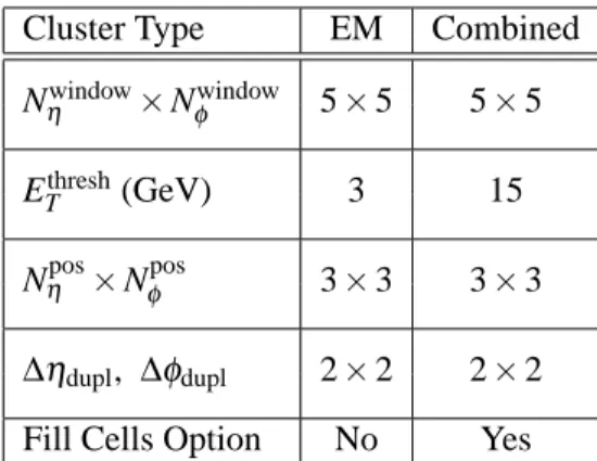
Cluster Type EM Combined
Nηwindow×Nφwindow 5×5 5×5
ETthresh(GeV) 3 15
Nηpos×Nφpos 3×3 3×3
∆ηdupl, ∆φdupl 2×2 2×2 Fill Cells Option No Yes
Table 2: Parameters for precluster (seed) finding using the sliding-window algorithm: Nηwindow×Nφwindow is the size of the window that is moved over the tower grid; ETthreshis the window energy threshold above which a precluster is built; Nηpos×Nφposis the size of the window that is used to compute the precluster position; and ∆ηdupl, ∆φdupl are the distances in η andφ used to detect duplicate preclusters. “Fill Cells Option” determines whether the precluster cells are taken directly from the cells within the sliding window, or if cluster filling is done as a separate step. Allη-φ numbers in this table are in tower units
∆φ and∆η, defined in Table 1.
Duplicate preclusters are then removed. If two preclusters have positions within∆ηdupl×∆φdupl, only the precluster with the largest transverse energy is kept; the other is removed.
Finally, the preclusters can optionally be filled with the cells that are encompassed by the sliding window. In this case, all cluster quantities such as the per-layer energies and positions are computed based on this set of cells. This is done for combined sliding-window clusters, for which a single set of clusters is ultimately built from these seeds, but not for EM clusters, for which clusters of many sizes can be constructed from the same seed. The latter clusters are filled in a separate step, described below.
Table 2 summarizes all parameters used in the precluster step.
2.1.3 EM Cluster Formation
Cells are assigned to EM clusters by taking all cells within a rectangle of size Nηcluster×Nφclustercentered on a layer-dependent seed position. Table 3 summarizes how this is performed: the middle layer is processed first, followed by the strips, the presampler, and the back. In the middle layer, the precluster barycenter positionηprecl,φpreclis used as the seed position. The barycenterηmiddle,φmiddle of the cells included from the middle layer is then computed. The strips layer is done next, using the barycenter from the middle layer as the seed position. For the strips, the size of the rectangle inφ varies depending on whether Nφwindow, the requested cluster size inφ, is less than 7. This is done in such a way that for a 5×5 cluster, if the seed is close to the boundary between two strips, then these two strips are included into the cluster in theφ direction, whereas if the seed is located in the middle of the strip, only one one strip is included. The barycenterηstrips,φstrips is computed from the cells in the strip layer. Finally, the PS and back layers are processed, using respectively the strip and middle layer barycenters as seed positions.
6)Special considerations apply at the edge of the calorimeter, where the tower with the maximum energy may be at the edge of the large sliding window (since the window is restricted so that it lies entirely within the calorimeter). If the smaller window is placed at the center of such a large window, it may miss most of the energy of the cluster. In such a case, when the large window is at the calorimeter edge, the smaller window may be centered on the tower with the largest energy.
Order Layer ∆ηcl(units of 0.025) ∆φcl(units of 0.025) Seed 1 Middle Nηcluster Nφcluster ηprecl,φprecl
2 Strips Nηcluster 6 or 8∗ ηmiddle,φmiddle
3 PS Nηcluster 6 or 8∗ ηstrips,φstrips
4 Back Nηcluster+1 Nφcluster ηmiddle,φmiddle
Table 3: Summary of cells included in the sliding window cluster for each EM calorimeter layer. Column 1 gives the order in which the layers are processed; columns 3 and 4 give the size∆ηcl×∆φclof the rectangle that is drawn around the seed position defining the cells that are included in the cluster; and column 5 gives the seed that is used for the each layer. (∗: either one or two cells inφ[of size 0.1] are used if the cluster size Nφwindowis less than 7; two cells inφ are used otherwise.)
Clusters of different Nηcluster×Nφclustersizes are built depending on the hypothesized particle type and the cluster’s location in the calorimeter. The optimization of the size is a compromise between two competing effects. The cluster should be large enough so that it contains most of the energy deposited by the particle in the calorimeter, thus limiting the effect of lateral shower fluctuations on the energy resolution. On the other hand, including more cells also means including more noise.
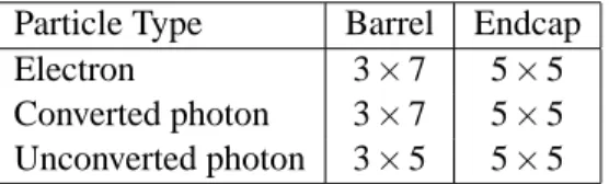
Particle Type Barrel Endcap
Electron 3×7 5×5
Converted photon 3×7 5×5 Unconverted photon 3×5 5×5
Table 4: Cluster size Nηcluster×Nφclusterfor different particle types in the barrel and endcap regions of the EM calorimeter.
Table 4 lists the cluster sizes used for different EM particle types in the barrel and endcap electro- magnetic calorimeters. In the barrel, showers from electrons are wider than those from photons because electrons interact more with upstream material, and also can emit bremsstrahlung photons. Since the magnetic field curves the electron trajectory in the φ direction, theφ size of the cluster is increased in order to contain most of the energy. Similarly, converted photons lead to electron-positron pairs that spread in theφ direction due to the magnetic field. In the endcaps, because the effect of the magnetic field is smaller, the cluster size is the same for all particle types. It is larger inηthan in the barrel because of the smaller physical cell size.
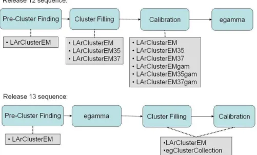
Technically, the actual construction of clusters of various sizes is not performed at the same time in the reconstruction chain in release 12 and subsequent releases. This is explained in Figure 1: in release 12, the clusters of various sizes are constructed before electron and photon (egamma) identification. This implies that, since cluster calibration occurs right after the clusters are built, every cluster size must be calibrated both as a potential electron or photon. This leads to an unnecessary duplication of calibrated clusters. This scheme was improved starting from release 13: the cluster construction and filling is done as a part of egamma identification. Thus, the particle type hypothesized for the cluster is known before cluster calibration.
2.2 Topological Clustering
The basic idea of topological clustering is to group into clusters neighboring cells that have significant energies compared to the expected noise. This results in clusters that have a variable number of cells, in contrast to the fixed-size clusters produced by the sliding-window algorithm (Sec. 2.1). Cluster growth starts at seed cells that have an energy significance, defined as signal to noise ratio, above a large threshold
Figure 1: Sequence of cluster building and egamma identification in releases 12 and 13. The blue boxes correspond to the steps described in this section, while the gray boxes list the cluster collections that are created. Note that egClusterCollection contains clusters of multiple sizes and calibrations.
tseed. Neighboring cells are added to the cluster if their significance is above a low threshold tcell; a neighboring cell can serve as an additional seed to expand the cluster if its significance is above a medium threshold tneighbor. The low threshold at the perimeter ensures that tails of showers are not discarded, while the higher thresholds for seeds and neighbors effectively suppress both electronics and pile-up noise.
The topological clustering algorithm consist of two steps: the cluster maker and the cluster splitter.
2.2.1 Cluster Maker
The algorithm to form topological clusters from a list of calorimeter cells (usually all cells, but may also be a subset of cells defined by a “region of interest,” such as that used in the high level trigger, or by the systems present in a beam test) consists of the following steps:
Finding seeds : Identify all cells with a signal to noise ratio above the (rather high) seed threshold tseed and put them into a seed list. Each seed cell forms a “proto-cluster.” The signal used for the threshold comparison can either be the cell energy or its absolute value. The noise is the expected RMS of the electronics noise for the current gain and conditions. Optionally, the expected contribution from pile-up may be added to the noise in quadrature (this is done by default)7). See Table 5 for the parameter values that are used.
Finding neighbors : All cells in the current seed list are ordered in descending order in signal to noise ratio. For each seed cell in turn, its neighboring cells are considered. If a neighboring cell has not been used as a seed so far, and its signal to noise ratio is above the neighbor threshold tneighbor, the cell is added to a neighbor seed list and included in the the adjacent proto-cluster. In the case where
7)It is foreseen that for real data, the noise measurement from zero-biased events in collision will be used as the expected noise.
the cell is adjacent to more than one proto-cluster, the proto-clusters are merged. If the signal to noise ratio is above the cell threshold tcell but below tneighbor, the cell is included only in the first adjacent proto-cluster, which is the one providing the more significant neighbor to this cell. Once all seed cells have been processed, the original seed list is discarded and the neighbor seed list becomes the new seed list. This procedure is repeated until the seed list is empty.
For this step, the signal is always defined as the absolute value of the energy|E|; the noise defi- nition is identical to that of the seed-finding step. The parameter values that are used are listed in Table 5. Note that tcell=0 implies that all cells neighboring a seed cell will end up in a cluster, regardless of their energies.
The definition of neighboring cells includes (usually) the eight surrounding cells within the same calorimeter layer. Optionally, the set of neighbors can also include cells overlapping partially in η and φ in adjacent layers and/or adjacent calorimeter systems. For a simple calorimeter with identical granularity in all layers, a typical cell would thus have ten neighbors with this option. In ATLAS, this number is often larger as the granularity varies between different calorimeter layers and regions. By default, this expanded definition of neighboring cells is used.
Finalize : The remaining proto-clusters (some of the original proto-clusters are merged with others) are sorted in descending order in ET and converted to clusters. Those with ET (optionally|ET|) less than a threshold are removed at this step.
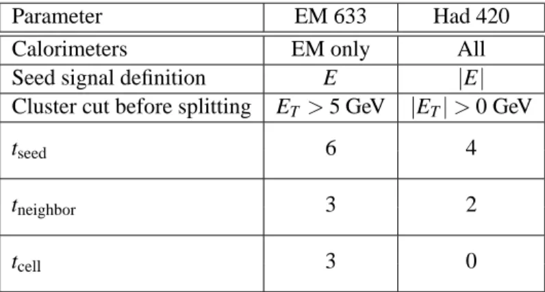
Parameter EM 633 Had 420
Calorimeters EM only All
Seed signal definition E |E|
Cluster cut before splitting ET >5 GeV |ET|>0 GeV
tseed 6 4
tneighbor 3 2
tcell 3 0
Table 5: Parameters used to build the two types of topological cluster available in the standard ATLAS reconstruction.
To summarize, topological clusters are seeded by cells with large signal to noise (above tseed), grow by iteratively adding neighboring cells (with signal to noise above tneighbor), and finish by including all direct neighbor cells on the outer perimeter (with signal to noise above tcell). In the standard ATLAS reconstruction, two types of topological clusters are built: the electromagnetic “633” clusters and the combined “420” clusters. The parameters defining these two cluster types are listed in Table 5. The
“633” cluster can be used to reconstruct EM clusters significantly higher than the noise with minimum fake rate. The “420 ” is optimized to find efficiently low energy clusters without being overwhelmed by noise. The cut on absolute energy ensures the noise constribution is symmetric.
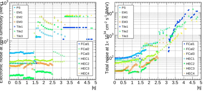
The cell-by-cell noise is computed by CaloNoiseTool [7, 8] and varies by many orders of magnitude over the entire detector. It also depends on the luminosity. Figure 2 shows the electronics noise (left) and total noise (right) for high luminosity (L =1034cm−2s−1). At high luminosity, the noise in the endcaps and forward region is dominated by pile-up.
Given the expected amount of noise, the number of clusters formed purely from noise can be pre- dicted as a function of the seed threshold. The expected number of purely noise clusters is given by the
η|
| 0 0.5 1 1.5 2 2.5 3 3.5 4 4.5 5
Electronic noise at zero luminosity (MeV)
102
103
FCal1 FCal2 FCal3 HEC1 HEC2 HEC3 HEC4 PS
EM1 EM2 EM3 Tile1 Tile2 Tile3
η|
| 0 0.5 1 1.5 2 2.5 3 3.5 4 4.5 5 (MeV)-1 s-2 cm34 10×Total noise at 1
102
103
104
FCal1 FCal2 FCal3 HEC1 HEC2 HEC3 HEC4 PS
EM1 EM2 EM3 Tile1 Tile2 Tile3
Figure 2: Per-cell electronics noise (left) and total noise at high luminosity (right), in MeV, for each calorimeter layer.
complementary error function of the seed threshold tseed: Nclus=FsignNcells
r2 π
Z∞ tseed
e−t2/2dt. (1)
Here, Fsign=1 for the “420” parameter set (which uses|E|to define cluster seeds) and 0.5 for “633”
(which uses E). Ncellsis the number of input cells; this is 187562 (all calorimeters) for “420” and 172160 (EM calorimeters only with|η|<2.5) for “633”.
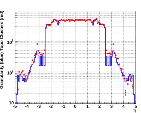
For the “420” cluster, 11.9 noise clusters are expected for the full set of 187652 cells. The distribution of these pure noise clusters as a function ofηstrictly follows the average granularity in each region, as shown in Figure 3.
The algorithm described so far is adequate for isolated signals, such as single particle beam tests. An early version of this algorithm with slightly different noise threshold choices was successfully used in the 2002 combined beam test with sections of the EM and hadronic endcap calorimeters [9].
2.2.2 Cluster Splitter
The ideal situation of isolated clusters is however not typical for most ATLAS events. Especially in the endcaps and forward calorimeters, clusters could grow to cover large areas of the detector if sufficient en- ergy is present between incident particles. However, even in the case of overlapping showers, individual particles may still be separable if they are far apart enough to form local maxima in the calorimeter.
The cluster splitting algorithm is designed for such situations and acts on the cells comprising the previously found topological clusters. The algorithm splits individual clusters, but the current implemen- tation processes all clusters at once.
Finding local maxima : A set of local maximum cells are defined as those clustered cells satisfying:
• E>500 MeV;
• Energy greater than that of any neighboring cell; and
-5 -4 -3 -2 -1 0 1 2 3 4 η5
Granularity (blue) Topo Clusters (red)
10 102
103
Figure 3: Average cell granularity (number of cells per∆η=0.1) as from the detector geometry (blue histogram) and as calculated from the distribution of topological clusters in simulated noise-only events (red points).
• Number of neighboring cells within the parent cluster above a threshold (default is≥4).
As described in the previous section, the definition of cell neighbors can either be restricted to a single calorimeter layer, or can also include cells from adjacent layers and subsystems. Generally, the choice used for cluster making should also be used here. It has been found that excluding cells from certain layers where no large maxima are expected, such as the presampler and the strips, suppresses the formation of noise clusters. By default, cells from the hadronic calorimeters are also excluded from forming local maxima. However, local maxima in the strips and the hadronic calorimeters are used if they don’t overlap with one of the primary local maxima inη andφ. In this way, hadronic clusters with significant energy in the EM calorimeters will be split based on their electromagnetic core, while those without significant EM activity can still be separated by coarser maxima in the hadronic calorimeters.
Once the list of local maxima is complete, the number of final clusters is fully determined: each local maximum will form exactly one cluster without the possibility of merging. Parent clusters without any local maximum cell will not be split.
Finding neighbors : Clusters are then grown around the local maxima as before, except that only the cells originally clustered are used, no thresholds are applied, and no cluster merging occurs. The local maxima list serves as the initial seed list. At each iteration, the current seed list is sorted in descending order in energy. All direct unused neighbors to the seed cells are added to a neighbor seed list and included in adjacent proto-clusters. In the case where a cell adjoins more than one proto-cluster, the two proto-clusters with the most energetic neighbors (i.e. the first two) will share the cell. Cells subject to sharing are removed again from the neighbor list and the proto-clusters and added to a shared cell list to be handled in the next step. Once all seed cells are processed, the original seed list is discarded and the neighbor seed list becomes the new seed list. This step is
iterated until the seed list is empty.
Shared cells : The shared cell list is next expanded by iteratively adding neighbors that are in the original cell set and which have not yet been assigned to any proto-cluster. These cells are associated with the two proto-clusters adjoining the original shared cell that they neighbor. Each cell in the expanded shared cell list is then added to its two adjoining proto-clusters with the weights
w1= E1
E1+rE2, w2=1−w1, r=exp(d1−d2), (2) where E1,2 are the energies of the two proto-clusters and d1,2are the distances of the shared cell to the proto-cluster centroids in units of a typical EM-shower scale (currently 5 cm). The weights give a rough estimate of the probability ratio for a given cell to belong to either cluster assuming the clusters originate from individual electromagnetic showers. In practice, the weights turn out to be close to either zero or one (they always sum to unity by definition), and thus the exact choice of the distance parameter is not critical.
Finalize : Each local maximum has now produced a proto-cluster. All parent clusters without a local maximum are added to the list of proto-clusters. They all are sorted in descending order in ET and converted to clusters.
At this point the topological clusters represent three dimensional energy blobs in the calorimeter that sometimes share cells on the border between them.
3 Performance of the Clustering Algorithms
Section 3.1 summarizes the generic properties (multiplicity per event, typical energy, cell content) of the two cluster types, while Secs. 3.2 and 3.3 present results specific to the two algorithms.
3.1 Typical Cluster Multiplicities, Energies, and Cell Content
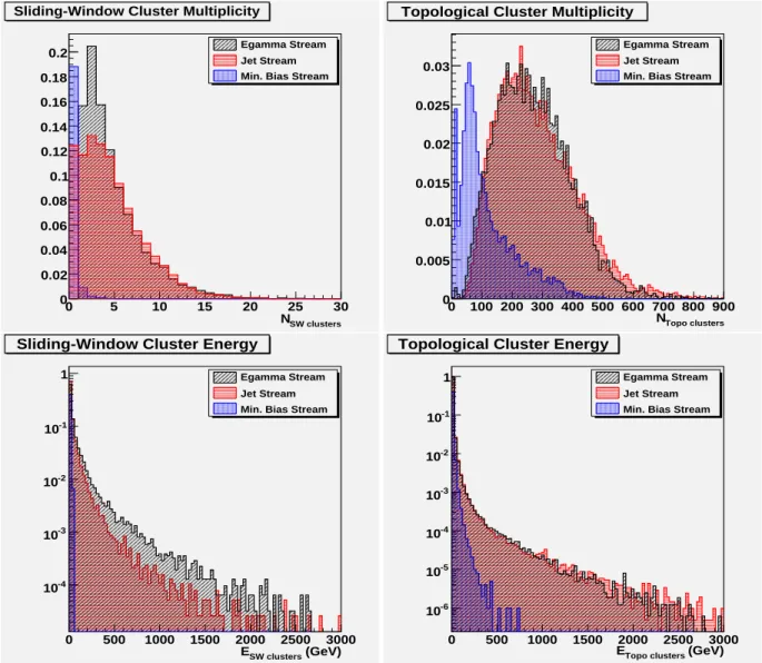
Figure 4 shows the distributions of cluster multiplicity and energy for 5×5 EM sliding-window and topo- logical 420 clusters, for typical ATLAS events from the egamma, jet, and minimum bias streams [10].
The multiplicity and energy distributions look similar for streams with high-pT physics content (egamma and jets), while they have lower mean values in other events such as from the minimum bias stream. While the typical number of EM sliding-window clusters peaks at 3 per physics event, the num- ber of 420 topological clusters peaks at around 250 per event.
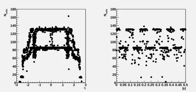
The number of cells as a function ofη andφin electromagnetic 5×5 clusters is shown in Figure 5.
Since the cluster has a fixed size, this is determined almost entirely by the detector geometry. Indeed, this number is more or less constant in the EM barrel, with two possible values depending on the φ barycenter position inside the strip compartment (one additional row inφ is included when the position is 0<φ<0.25 or 0.75<φ<1 in strip cell units). The number of cells decreases withηin the endcaps because the granularity of strip cells increases withη; thus fewer strip cells are included in the constant 5×5 cluster size. The spread near|η| ∼1.4 coincide with the barrel-endcap overlap region.
Figure 6 shows the number of cells in 420 topological clusters. These clusters are of variable size, depending mostly on the energy of the incoming particle: more energetic particles produce larger showers and thus larger clusters.
SW clusters
N
0 5 10 15 20 25 30
0 0.02 0.04 0.06 0.08 0.1 0.12 0.14 0.16 0.18 0.2
Sliding-Window Cluster Multiplicity
Egamma Stream Jet Stream Min. Bias Stream
Sliding-Window Cluster Multiplicity
Topo clusters
N
0 100 200 300 400 500 600 700 800 900 0
0.005 0.01 0.015 0.02 0.025 0.03
Topological Cluster Multiplicity
Egamma Stream Jet Stream Min. Bias Stream
Topological Cluster Multiplicity
(GeV)
SW clusters
E
0 500 1000 1500 2000 2500 3000 10-4
10-3
10-2
10-1
1
Sliding-Window Cluster Energy
Egamma Stream Jet Stream Min. Bias Stream
Sliding-Window Cluster Energy
(GeV)
Topo clusters
E
0 500 1000 1500 2000 2500 3000 10-6
10-5
10-4
10-3
10-2
10-1
1
Topological Cluster Energy
Egamma Stream Jet Stream Min. Bias Stream
Topological Cluster Energy
Figure 4: Electromagnetic 5×5 sliding-window cluster (left) and 420 topological cluster (right) multi- plicities (top) and energies (bottom), shown for three data streams: egamma, jet, and minimum bias.
-3 -2 -1 0 1 2 η3
cellsN
0 20 40 60 80 100 120 140 160 180
φ|
| 0 0.05 0.1 0.15 0.2 0.25 0.3 0.35 0.4 0.45 0.5
cellsN
0 20 40 60 80 100 120 140 160 180
Figure 5: Number of cells in electromagnetic 5×5 clusters as a function ofη(left) and|φ|(right) with
|φ|<0.5 in strip cell units.
(GeV) ET
0 50 100 150 200 250 300 350 400 450 500
CellN
100 200 300 400 500 600 700
Figure 6: Number of cells in 420 topological clusters as a function of the cluster transverse energy, from the egamma data stream.
3.2 Sliding-Window Clustering
3.2.1 Efficiency, Fake Rate, and Duplicate Clusters
Single particle samples are used to study the sliding window clustering efficiency and the rates of fake and duplicate clusters.
The clustering efficiency is defined as the ratio of the number of events where at least one cluster is reconstructed over the total number of events:
ε= N(ncluster>0)
Ntotal . (3)
This formula is correct provided that the fake rate is negligible, which is demonstrated to be the case below.
Fake and duplicate clusters are seen in events where more than one cluster is reconstructed in a single particle sample. Fake clusters are clusters formed purely from noise (only electronic noise is considered here), and are more or less uniformly distributed in theη,φplane. Duplicate clusters often arise from real physics processes: for electrons, duplicate clusters can originate from the emission of bremsstrahlung photons, and for photons, they can arise from conversions. When this occurs, the secondary particle can produce an additional cluster very close to the cluster from the original particle. If the distance between two clusters∆R<0.3, the clusters are considered to be duplicates; otherwise, one of the two clusters is considered to be a fake.
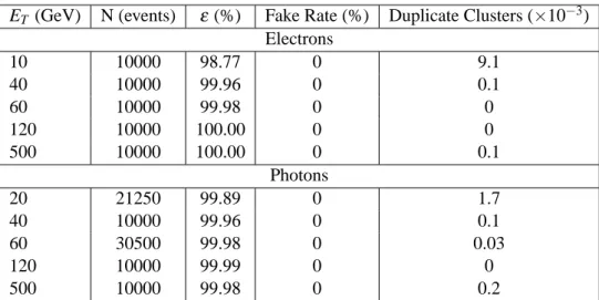
Table 6 gives the clustering efficiency and the rates of fake and duplicate clusters for the EM sliding window algorithm applied to single electron and photon samples of various transverse energies. As expected, the clustering efficiency rises with the energy
ET (GeV) N (events) ε (%) Fake Rate (%) Duplicate Clusters (×10−3) Electrons
10 10000 98.77 0 9.1
40 10000 99.96 0 0.1
60 10000 99.98 0 0
120 10000 100.00 0 0
500 10000 100.00 0 0.1
Photons
20 21250 99.89 0 1.7
40 10000 99.96 0 0.1
60 30500 99.98 0 0.03
120 10000 99.99 0 0
500 10000 99.98 0 0.2
Table 6: Clustering efficiency and rates of fake and duplicate clusters for the EM sliding window algo- rithm applied to single electron and photon samples of various transverse energies.
The rate of duplicate clusters decreases as the energy increases (except at very high energy). This is because the opening angle between the two particles (electron-photon or electron-positron) is larger at lower energy, giving some separation between the clusters. As the energy increases, the angle be- comes smaller than the∆ηdupl and∆φdupl cuts (see Table 2), and thus the number of duplicate clusters decreases8). At very high energy (ET =500 GeV), catastrophic interactions of electrons and photons with matter can create (legitimate) closely-spaced clusters, which are counted as duplicates in the table.
8)Computing these numbers, a bug was discovered in the simulation in the computation of the cell identifier. As a conse- quence, some energy can be assigned to the wrong cell aroundη=0, creating fake duplicate clusters for incoming particles of sufficient energy (>∼500 GeV). This effect is subtracted from the numbers quoted in the table.
3.2.2 Sliding Window Clustering Parameters
As described in Sec. 2.1, the sliding window clustering algorithm consists of three steps: tower building, precluster (seed) finding, and cluster filling. The tower building parameters, given in Table 1, are deter- mined by the geometrical specifications and granularities of the calorimeters used. The parameters for preclustering quoted in Table 2 are determined by typical shower sizes in the calorimeter.
EM preclusters (seeds) are always found by moving a 5×5 window over the array of towers, though clusters of other sizes may be built later. This is sufficient for the standard electron and photon reconstruc- tion, but is not adequate for other applications, such as recovering energy lost to bremsstrahlung. Each such application may require building additional clusters with retuned parameters in order to achieve optimal performance.
3.2.3 Nearby Clusters and Energy Sharing
Sliding-window clusters that are close together can have cells in common. By default, the sliding-window cluster reconstruction simply ignores such cases and assigns the entire energy of the shared cells to all overlapping clusters. The energies of shared cells are thus counted multiple times.
An optional algorithm is available to handle properly sharing cells between clusters. When this is used, if a cell is shared by N clusters, its energy is added to each of the clusters with the following weights:
wi,j= Ej
ΣNk=1Ek, (4)
for a cell i in a cluster j.
Energy sharing is illustrated in Figure 7, where results from a 50 GeV single photon sample are shown. For the case in which the energy sharing algorithm is not used, the total reconstructed energy can be larger than initial photon energy due to double counting of cells in overlapping clusters reconstructed around the e+e−pair created by photon conversions. After the energy sharing algorithm has been applied, the total energy becomes comparable to the initial photon energy, demonstrating that the double-counting is gone.
3.3 Topological Clustering
3.3.1 Nearby Clusters and Energy Sharing
Two clusters may share some cells in the border region between them, as described in Sec. 2.2. The cluster splitting algorithm ensures that the weights given a cell shared between multiple clusters add to unity; thus no double counting of energy occurs.
3.3.2 Noise Uncertainty
Since all thresholds for topological clustering are relative to the expected amount of noise, both from electronics and pile-up, uncertainties in these numbers have a direct effect on the reconstruction effi- ciency of the clustering algorithm. Such uncertainties can result in an increase in the number of fake clusters (especially if the thresholds are low) and also lower clustering efficiency and more bad cells included in clusters, when the incoming particle energy becomes close to the thresholds.
To illustrate the first issue, consider the effect that a 10% noise variation in all cells (a very unlikely scenario) would have on building topological clusters with the 420 and 633 parameters. The variation in noise will affect the clusters with low threshold much more than those with higher thresholds.
Figure 8 shows Nclusfor the 420 and 633 parameter sets for a 10% noise variation (3.6<tseed<=4.4 for 420 and 5.4<tseed<=6.6 for 633). For the 420 case, the 10% noise variation shifts the mean number
All Clusters Energy (GeV)
10 20 30 40 50 60 70 80 90 100
entries/bin
1 10 102
103
without energy sharing with energy sharing
Figure 7: Reconstructed total energy from 50 GeV single photon events without energy sharing (red dashed histogram) and with energy sharing (blue solid histogram). No standard cluster corrections have been applied.
of purely noise clusters per event from a nominal value of 12 to 2 (for an overestimate of the noise) or 60 (for an underestimate). For the 633 case, the number of noise clusters per event is always very small, even in the presence of noise uncertainties.
Summary
The two clustering algorithms used in the ATLASATHENAreconstruction releases 12 and 13 have been described and their performance summarized. Several improvements are expected to the sliding-window algorithm in future releases. The clustering parameters can be optimized to better handle situations with very low energy particles or with more than one single particle (electrons that emit bremsstrahlung photons, or converted photons). Duplicate clusters also need to be removed. The number of strip cells included in the clusters may also be reconsidered.
The hadronic “‘420” topological clusters are now widely used and validated. The electromagnetic
“633” clusters were studied as an alternative to the EM sliding-window clusters, but are not currently used in the reconstruction of any physics object. This cluster type will thus be removed from the standard reconstruction unless some use is found for it.
noise) σ Seed threshold ( 3.5 3.6 3.7 3.8 3.9 4 4.1 4.2 4.3 4.4 4.5 due to noise420 topo clustersN
0 10 20 30 40 50 60 70 80
erfc(x) Single Particle Data
420 Topo clusters
noise) σ Seed threshold (
5.4 5.6 5.8 6 6.2 6.4 6.6
due to noise633 topo clustersN
10-5
10-4
10-3
10-2
633 Topo clusters
Figure 8: Number of noise clusters vs. the seed threshold tseedfor the 420 (left) and 633 (right) parameter sets as predicted by Eq. 1. On the left plot, the measured numbers of clusters in a 100 GeV single electron sample obtained with tseed=3.6, 4, and 4.4 are superimposed.
References
[1] The ATLAS Collaboration, The ATLAS Experiment at the CERN Large Hadron Collider, 2008, submitted to JINST (2008).
[2] The ATLAS Collaboration, Liquid Argon Calorimeter Technical Design Report, 1996, CERN/LHCC/96-41.
[3] The ATLAS Collaboration, Tile Calorimeter Technical Design Report, 1996, CERN/LHCC/96-42.
[4] C. Adam-Bourdarios, S. Snyder et al, EM Calorimeter Calibration and Performance, 2008, CSC- EG-06.
[5] P. Schacht et al, Performance of Overall Calorimetry Energy Reconstruction: Hadronic Calibration H1, Topo Cluster Classification, 2008, CSC-CALO-02.
[6] The ATLAS Collaboration, Electromagnetic Reconstruction in Liquid Argon Calorimeter at CTB, 2008, Reference not available yet..
[7] W. Lampl et al, Digitization of LAr Calorimeter for CSC simulations, 2007, ATL-LARG-PUB- 2007-011.
[8] M.Lechowski, Test of the ‘Little Higgs’ Model in ATLAS at LHC, and Simulation of the Digitiza- tion of the Electromagnetic Calorimeter. (In French), 2005, CERN-THESIS-2005-042.
[9] C.Cojocaru et al, Nucl. Instrum. Meth. A531 (2004) 481–514.
[10] J.F.Arguin et al, Data Streaming in ATLAS, 2007, ATL-COM-GEN-2007-004.