Technische Universit¨ at M¨ unchen
Max-Planck-Institut f¨ ur Physik (Werner-Heisenberg-Institut)
Techniques to distinguish between electron and photon induced events using segmented germanium detectors
Kevin Kr¨oninger
Vollst¨andiger Abdruck der von der Fakult¨at f¨ur Physik der Technischen Universit¨at M¨unchen zur Erlangung des akademischen Grades eines
Doktors der Naturwissenschaften (Dr. rer. nat.) genehmigten Dissertation.
Vorsitzender: Univ.-Prof. Michael Ratz Pr¨ufer der Dissertation:
1. Hon.-Prof. Allen C. Caldwell, Ph.D 2. Univ.-Prof. Lothar Oberauer
Die Dissertation wurde am 26.04.2007 bei der Technischen Universit¨at M¨unchen eingereicht und durch die Fakult¨at f¨ur Physik am 05.06.2007 angenommen.
Abstract
Two techniques to distinguish between electron and photon induced events in germanium detectors were studied: (1) anti-coincidence requirements between the segments of seg- mented germanium detectors and (2) the analysis of the time structure of the detector response.
An 18-fold segmented germanium prototype detector for the GERDA neutrinoless double beta-decay experiment was characterized. The rejection of photon induced events was measured for the strongest lines in 60Co,152Eu and 228Th. An accompanying Monte Carlo simulation was performed and the results were compared to data. An overall agree- ment with deviations of the order of 5-10% was obtained. The expected background index of theGERDAexperiment was estimated.
The sensitivity of the GERDAexperiment was determined. Special statistical tools were developed to correctly treat the small number of events expected.
The GERDA experiment uses a cryogenic liquid as the operational medium for the germanium detectors. It was shown that germanium detectors can be reliably operated through several cooling cycles.
Zusammenfassung
Es wurden zwei Techniken zur Unterscheidung von Elektron- und Photon-induzierten Ereignissen in Germanium-Detektoren untersucht: (1) Anti-Koinzidenzen zwischen den Segmenten segmentierter Germanium-Detektoren und (2) die Analyse der Zeitstruktur der Detektor-Antwortfunktion.
Ein 18-fach segmentierter Prototyp-Detektor f¨ur das GERDAExperiment zu neutri- nolosem Doppelbeta-Zerfall wurde untersucht und charakterisiert. Insbesondere wurde die Unterdr¨uckung Photon-induzierter Ereignisse f¨ur die st¨arksten Linien von60Co,152Eu und228Th gemessen. Die Ergebnisse wurden mit den Resultaten einer begleitenden Monte Carlo Studie verglichen. Die Simulationen beschreiben die Daten mit Abweichungen von etwa 5-10%. Der erwartete Untergrund desGERDAExperiments wurde abgesch¨atzt.
Spezielle statistische Verfahren, welche die kleine Anzahl von erwarteten Ereignissen ber¨ucksichtigen, wurden entwickelt um die Sensitivit¨at des Experiments auf neutrinolosen Doppelbeta-Zerfall abzusch¨atzen.
DasGERDAExperiment wird Germanium Detektoren direkt in einer Kryofl¨ussigkeit betreiben. Es konnte gezeigt werden, dass Detektoren ohne eine Beeintr¨achtigung der Leistung ¨uber mehrere Kalt-Warm-Zyklen betrieben werden k¨onnen.
Contents
1 Introduction 1
2 Neutrinoless double beta-decay in the SM 5
2.1 Electro-weak interaction and neutrinos . . . 5
2.1.1 From weak to electro-weak interaction . . . 5
2.1.2 Leptons and the Standard Model . . . 6
2.2 Neutrino oscillations . . . 6
2.2.1 Neutrino oscillation parameterization . . . 7
2.2.2 Solar neutrinos . . . 8
2.2.3 Summary of experimental results . . . 10
2.3 Neutrino mass terms and measurements . . . 12
2.3.1 Neutrino mass terms . . . 12
2.3.2 Neutrino mass measurements . . . 13
2.4 Double beta-decay . . . 14
2.4.1 Extraction of mass parameters . . . 17
2.4.2 Experimental considerations . . . 17
2.4.3 Search for neutrinoless double beta-decay of76Ge . . . 19
3 The GERDA experiment 21 3.1 Concept . . . 21
3.2 Location of the experiment - LNGS . . . 23
3.3 Technical realization . . . 24
3.3.1 Active detector components . . . 24
3.3.2 Water tank and cryogenic vessel . . . 26
3.3.3 Super-structure and clean room . . . 27
3.3.4 Electronics and data acquisition system . . . 27
3.4 Status of the experiment . . . 27
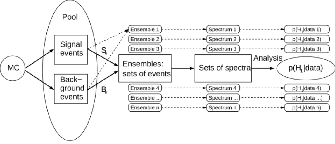
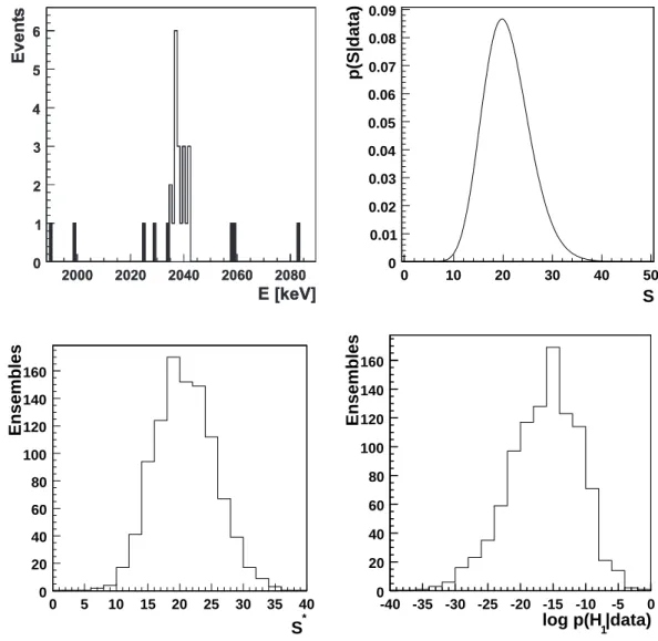
4 Sensitivity of the GERDA experiment 29 4.1 Spectral analysis . . . 30
4.1.1 Hypothesis test . . . 30
4.1.2 Signal parameter estimate . . . 32
4.1.3 Setting limits on the signal parameter . . . 33 i
ii CONTENTS
4.2 Ensemble tests . . . 33
4.3 Result . . . 34
4.3.1 Expected spectral shapes and prior probabilities . . . 34
4.3.2 Ensembles . . . 36
4.3.3 Sensitivity . . . 36
4.3.4 Influence of the prior probabilities . . . 40
4.3.5 Studies on the stability of the method . . . 41
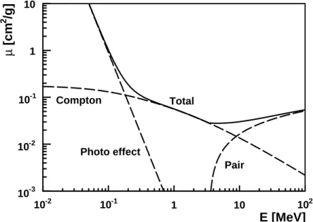
5 Germanium detectors 43 5.1 Interactions of electrons, positrons and photons with matter . . . 43
5.1.1 Electrons and positrons . . . 43
5.1.2 Photons . . . 44
5.2 Semiconductor (germanium) detectors . . . 45
5.2.1 Working principle . . . 45
5.2.2 Germanium semiconductor detectors . . . 47
5.2.3 Electric fields . . . 47
5.3 Signal development in (germanium) detectors . . . 48
5.3.1 Crystal axes . . . 49
5.4 Germanium detector properties . . . 50
5.4.1 Operation temperature . . . 50
5.4.2 Energy resolution . . . 50
5.5 Segmented germanium detectors . . . 50
5.6 Signal amplification and read out . . . 52
6 Signatures and background rejection 53 6.1 Signal process and signature . . . 53
6.2 Background sources . . . 53
6.2.1 Internal background sources . . . 54
6.2.2 External background sources . . . 54
6.3 Classification of signal and background signatures . . . 55
6.4 Background rejection techniques . . . 56
7 Background rejection using segmented detectors 59 7.1 MaGe - theGERDAMonte Carlo framework . . . 59
7.1.1 Simulation of theGERDAgeometry . . . 60
7.1.2 Simulation of test stands . . . 61
7.2 Selected background processes . . . 61
7.3 Spatial distribution of energy deposition . . . 61
7.4 Multiplicities and suppression factors . . . 64
8 Background rejection using pulse shape analysis 69 8.1 Analysis methods . . . 69
8.1.1 Likelihood discriminant method . . . 69
8.1.2 Library method . . . 71
CONTENTS iii
8.1.3 Neural network method . . . 71
9 GERDA test facility 73 9.1 Cryoliquid-submersion test stand . . . 73
9.1.1 Cooling cycle . . . 74
9.1.2 Results . . . 75
9.2 Phase II prototype detectorSiegfried . . . 76
9.3 Siegfried Monte Carlo simulation . . . 79
10Siegfried measurements and data sets 81 10.1 Detector characterization measurements . . . 81
10.2 Segmentation study . . . 82
10.3 Pulse shape analysis . . . 82
10.3.1 Event selection . . . 83
10.4 Full event display . . . 85
11Siegfried results 87 11.1 Prototype detector characterization . . . 87
11.1.1 Leakage current and capacitance . . . 87
11.1.2 Bias voltage . . . 87
11.1.3 Cross-talk . . . 87
11.1.4 Segment-core correlation . . . 90
11.1.5 Linearity . . . 92
11.1.6 Energy resolution . . . 92
11.1.7 Segment scan . . . 92
11.1.8 Drift anisotropy . . . 93
11.1.9 Mirror charges and position sensitivity . . . 95
11.1.10 Summation of segment energies . . . 96
11.2 Electron/photon distinction . . . 98
11.2.1 Background estimate . . . 98
11.2.2 Rejection of photon induced events . . . 98
11.2.3 Segmentation scheme evaluation . . . 100
11.2.4 Threshold effects . . . 102
11.2.5 Geometry dependence of results . . . 102
11.2.6 Background . . . 103
11.2.7 Data to Monte Carlo comparison . . . 103
11.3 Pulse shape analysis . . . 107
11.3.1 Monte Carlo simulation . . . 107
11.3.2 Results . . . 109
11.3.3 Selection of electron-like events and discrimination against photon-like events . . . 109
11.3.4 Selection of single-site events and discrimination against multi-site events . . . 112
11.3.5 Application to the228Th data set . . . 112
iv CONTENTS
12 Background estimate 115
12.1 Materials and masses . . . 115 12.2 Expected background index . . . 117
13 Conclusions and outlook 119
Bibliography 125
Chapter 1
Introduction
Since its postulation by Pauli in 1931 the neutrino was assumed to be a very light (mass- less in the Standard Model) and chargeless Dirac particle. Early on it was recognized that the neutrino could also be a Majorana particle, i.e., its own anti-particle. The obser- vation of neutrino oscillations, rewarded with the Nobel Prize in 2002, gave evidence for finite masses of the neutrinos. Because only mass differences can be inferred from these observations, the absolute neutrino mass scale is still unknown. The question whether the neutrino is a Dirac or Majorana particle is also still open.
Nowadays, three classes of experiments aim to measure the neutrino mass scale. The exact determination of the end point energy of the spectrum of tritium beta-decays can be used to calculate the mass of the electron neutrino; structure formation in the uni- verse can be used to set limits on the sum of the neutrino masses; finally, the observation of neutrinoless double beta-decay could give information about a possible mass of the neutrino. The latter would also prove that the neutrino is a Majorana particle. So far, all three approaches could only set upper limits on the neutrino mass of the order of 1-2 eV.
Searches for neutrinoless double beta-decay reach back to the 1950ies. The most strin- gent limits come from experiments built to search for neutrinoless double beta-decay of the germanium isotope76Ge. Germanium is a semiconductor and can therefore be used as source and detector simultaneously. The sensitivity of previous experiments was lim- ited not only by the exposure but also by background which was dominated by external γ-radiation [1, 2].
The GERmanium Detector Array,GERDA[3], is a new experiment which is built to search for neutrinoless double beta-decay of 76Ge. It is currently being installed in the Hall A of the INFN Gran Sasso National Laboratory (LNGS), Italy. The background index aimed at is two orders of magnitude below that of recent experiments. With 100 kg·years exposure this will result in a sensitivity to the effective Majorana neutrino mass of about 200 meV. The background reduction is accomplished by a reduced amount of background producing material close to the detectors, a large passive shielding and, for the second phase of the experiment, the usage of segmented germanium detectors.
1
2 CHAPTER 1. INTRODUCTION The main goal of this thesis is to evaluate the potential of segmented germanium de- tectors to distinguish electron induced events from events induced by multiply scattered photons. The second goal is to study the operation of germanium detectors submerged in a cryogenic liquid.
Four aspects are investigated in particular with respect to the distinction between electrons and photons:
1. An estimate of the sensitivity of GERDA to neutrinoless double beta-decay for different background scenarios. Special statistical analysis tools were developed for the treatment of the small number of expected events.
2. The evaluation of the potential of segmented germanium detectors to distinguish electron induced events from events induced by multiply scattered photons using segment coincidences. The impact on the background reduction in the GERDA experiment was estimated using Monte Carlo techniques.
3. The characterization of a segmented prototype detector. A test stand for a segmented prototype detector for the second phase of theGERDAexperiment was built. Data were taken with this detector and analyzed with respect to the distinction between electrons and photons using segment coincidences. The results were compared to the predictions from a Monte Carlo simulation.
4. The evaluation of the potential of segmented germanium detectors to distinguish electron induced events from events induced by multiply scattered photons analyzing the time structure of the detector response. Data were taken with the prototype detector and the detector response was analyzed. Three different analysis methods were developed and the results compared.
The studies are performed in the context of the second phase of the GERDAexperi- ment. Chapter 2 summarizes today’s picture of neutrinos in the Standard Model and the double beta-decay processes. The concept and the technical realization of the GERDA experiment are described in Chapter 3. A spectral analysis technique developed to esti- mate the sensitivity of the experiment is introduced in Chapter 4. The operation principle and the development of the electrical signals of germanium detectors is discussed in Chap- ter 5. The main background sources forGERDAare summarized in Chapter 6 where the signatures of the signal and background processes are discussed. Monte Carlo simulations of the introduced processes are presented in Section 7.1.
Photons in the MeV-energy region typically scatter multiple times inside germanium and deposit their energy over a range of several centimeters. In contrast, electrons in the same energy region deposit their energy on a millimeter scale. Electrons and photons can thus be distinguished by determining the spatial distribution over which energy is deposited. This can be done by using segmented detectors (Chapter 7), or by analyzing the time structure of the detector response (Chapter 8).
3 The experimental setup of the prototype detector and the data sets are described in the second part of Chapter 9 and in Chapter 10. The simulation of the test stand is also described Chapter 9. The data taken with the prototype detector were compared to Monte Carlo data in order to verify the Monte Carlo simulation. The results are presented in Chapter 11.
A second, unsegmented germanium detector was operated while being submerged in liquid nitrogen or argon. The setup and the results are described in Chapter 9. It is shown that this mode of operation is feasible.
In Chapter 12 the developed background reduction techniques are applied to Monte Carlo data in order to estimate the background index of theGERDA experiment. Con- clusions and a summary are given in the last chapter.
4 CHAPTER 1. INTRODUCTION
Chapter 2
Neutrinoless double beta-decay in the framework of the Standard
Model
2.1 Electro-weak interaction and neutrinos
The neutrino was postulated by Pauli in 1931 as a very light and chargeless particle which would restore energy conservation in nuclear beta-decay. Fermi’s description of the inter- action of neutrinos, the weak interaction, was developed in the 1930ies and could explain many phenomena observed in nature. These range from the spectra in the mentioned nuclear beta-decay to the decay kinematics of muon and tau leptons. Although part of a successful theory it was not before 1953 that (anti-)neutrinos were first observed by Cowen and Reines in a reactor experiment [4].
Since then, many observations and modifications of the existing theory have led to a unified description of electro-magnetism and the weak interaction. TheStandard Model of Particle Physics(SM) is based on theelectro-weak andstrong forces. It was developed by Glashow, Salam and Weinberg [5–7] and so far gives a valid description of the interactions of its constituents, including neutrinos. A variety of measurements, partially motivated by theoretical predictions, confirm the validity of the model. The measurements include the observation of parity violation by Wu in 1957 [8] and the first direct observation of massive intermediate gauge bosons at CERN in 1983 [9, 10].
2.1.1 From weak to electro-weak interaction
Fermi’s ansatz for the description of neutrino interactions was inspired by quantum elec- trodynamics (QED) assuming a point-like vector-vector Lorentz-invariant amplitude. Al- though successful in many respects, Fermi’s model of the weak interaction is an effective, low-energy theory. The theory violates unitarity at high energies and fails to explain the experimental observation of parity violation. Two major modifications of the theory
5
6 CHAPTER 2. NEUTRINOLESS DOUBLE BETA-DECAY IN THE SM solved these problems: the introduction of intermediate vector bosons by Yukawa (1938) and Schwinger (1957), and the assumption of a V–A current. In this framework only the left-handed component of the neutrino field participates in the weak interaction. Parity is maximally violated.
A unification of electro-magnetism and the weak interaction was necessary in order to accommodate these two modifications and explain the experimental data. The electro- weak interaction reflects aSU(2)L×U(1)Y symmetry, where the subscriptLrefers to the weak isospin current which only couples to left-handed fermions. The subscript Y refers to the weak hypercharge current which couples to left- and right-handed fermions. Three massive gauge bosons, the charged W± and the neutral Z0, and one massless photon, γ, mediate the force. The former two only couple to the left-handed components of the lepton fields, whereas the Z0 and the photon couple to left- and right-handed fields. The observable W± bosons are combinations of the two charged fields from the SU(2)L sym- metry, whereas theZ0and the photon are mixtures of the two neutral fields emerging from theSU(2)LandU(1)Y symmetries. The latter mixing is described by the Weinberg angle.
2.1.2 Leptons and the Standard Model
Three types, or flavors, of charged leptons are known: electron (e), muon (µ) and tau (τ).
The number of flavors is not predicted by the Standard Model. From the measurement of the width of the Z0 boson at the SLC and LEP colliders [11] it was inferred that only three types of light neutrinos exist. Each charged lepton is assigned a neutrino partner.
The pair is referred to as a generation and interpreted as a left-handed doublet (under a SU(2) transformation), ¡
νLl, lL¢
, with l = e, µ, τ. A right-handed singlet lR of the charged lepton accompanies the doublet. Leptons from different generations couple with the same strength, but differ in mass. Although not required by the Standard Model, the lepton number, L, is found to be conserved family-wise1, i.e., the number of leptons of a certain flavor, Ll, is the same in the initial and final state of an interaction (∆Ll = 0).
No evidence for total lepton number violation has been found so far (see review article in [12]).
2.2 Neutrino oscillations
The picture of neutrinos was revised after the observation of neutrino oscillations. If neutrinos are massive particles and their flavor (or weak interaction) eigenstates do not coincide with their mass eigenstates, neutrinos can change their flavor. The first evidence that the physics of neutrinos deviates from SM assumptions came from the measurement of the solar neutrino flux and was known as thesolar neutrino problem[13]. Later, theat- mospheric neutrino anomaly, a measured deficit of muon neutrinos from the atmosphere, could also not be explained in the context of the SM.
1Not taking into account the neutrino oscillations discussed later.
2.2. NEUTRINO OSCILLATIONS 7 In the following a mathematical description of neutrino oscillations is introduced. An overview of the solar neutrino problem and its interpretation are presented as an example for the compelling experimental evidence for neutrino oscillations. A summary of recent experimental results is given at the end of this section. A detailed overview of neutrino mixing is given in e.g., [14].
2.2.1 Neutrino oscillation parameterization
If neutrinos are massive and the neutrino flavor eigenstates, να (α = e, µ, τ, . . . 2), do not coincide with the neutrino mass eigenstates,νj (j=1, 2, 3,. . . ), neutrinos of a specific flavorα can be described as a combination of mass eigenstates:
|ναi=X
j
Uαj∗ |νji , (2.1)
whereU is a unitary matrix referred to as the Pontecorvo-Maki-Nakagawa-Sakata (PMNS) matrix.
Using Schr¨odinger’s equation the time evolution of the neutrino can be calculated. A neutrino produced with the flavorα which has traveled a distance Lcan be described as
|να(L)i ≈X
j
Uαj∗ e−i(m2j/2E)L|νji , (2.2)
wheremj is the mass of the jth mass eigenstate andE is the average energy of all mass eigenstates. Inverting Equation (2.1) and re-inserting it into Equation (2.2) results in
|να(L)i ≈X
β
X
j
Uαj∗ e−i(m2j/2E)LUβj
|νβi . (2.3)
The probability to find the neutrino in a flavor state |νβi after it traveled a distance L is |hνβ να(L)i|2. The observation of such a transition implies that the lepton number is not conserved family-wise. The probability for a change of neutrino flavor can easily be calculated for the case of two neutrino flavors. Solar neutrino oscillations are given as an example later.
Two neutrino case: Assuming only two flavors (να, νβ) and two mass eigenstates (ν1,ν2), the unitary matrix U in Equation (2.1) is a two-dimensional rotation matrix
U =
· cosθ sinθ
−sinθ cosθ
¸
, (2.4)
2Allowing for more than three flavors, e.g., for sterile or very heavy neutrinos.
8 CHAPTER 2. NEUTRINOLESS DOUBLE BETA-DECAY IN THE SM whereθis the (one) mixing angle. Forθ= 0◦the flavor eigenstates do not mix, i.e., flavor and mass eigenstates are identical. For finiteθ the probability for the neutrino to change flavor, p(να →νβ), is
p(να →νβ) = sin22θsin2 µ
∆m212 L 4E
= sin22θsin2 µ
1.27∆m212[eV2] L[km]
E [GeV]
, (2.5)
with ∆m212 =m21−m22. The first line is in natural, the second line is in real units. The probability to change flavor depends on the mass squared difference of the mass eigen- states, the average neutrino energy and the distance the neutrino travels. The neutrino flavor changes periodically with the distanceL, hence the name neutrino oscillations. Note that for neutrino oscillations to be possible, the mixing angle θ has to be different from zero and at least one of the two mass terms has to be greater than zero.
Three neutrino case: Assuming three neutrino flavors (νe,νµ,ντ) the unitary matrix U becomes a 3×3 matrix. A common parameterization is
U =h 1 0 0
0 c23 s23 0 −s23 c23
i
×
· c13 0 s13e−iδ
0 1 0
−s13eiδ 0 c13
¸
×h c12 s12 0
−s12 c12 0
0 0 1
i
×
· eiα1/2 0 0
0 eiα2/2 0
0 0 1
¸ , (2.6) where sij = sinθij and cij = cosθij represent the sines and cosines of the three mixing angles. δ,α1 andα2 areCP-violating phases. The latter two are only of importance if the neutrino is its own anti-particle (see next section). In total there are six (eight) free pa- rameters to describe neutrino oscillations: three mixing angles, two mass differences (the third one is constrained) and one (three)CP-phase(s). The observed neutrino oscillations can be described as two flavor oscillations (see Section 2.2.3) in most cases.
The calculations presented previously are applicable for oscillations in the absence of matter and referred to as vacuum oscillations. The probability for changing flavor is altered in matter due to scattering processes viaW±- (onlyνe) andZ0-exchange (allν’s) [15, 16].
This is referred to as the Mikheyev-Smirnov-Wolfenstein (MSW) effect. It accounts e.g., for the large reduction in the solar neutrino flux.
2.2.2 Solar neutrinos
The sun produces large fluxes of electron neutrinos in a chain of processes. The energy dependent flux of neutrinos produced in the participating reactions are shown in Figure 2.1 as predicted by theStandard Solar Model(SSM) [17]. The proton-proton fusion (ppchain), p+p →D+e++νe, produces the largest flux of neutrinos with energies of up to about 0.42 MeV. The 7Be-process, 7Be +e− →7Li +νe, produces mono-energetic neutrinos of 0.86 MeV. Neutrinos with energies of up to 14.06 MeV are emitted in the decay of 8B,
8B→8Be +e++νe.
2.2. NEUTRINO OSCILLATIONS 9 In 1968, Ray Davis Jr. and collaborators were the first to measure the solar neutrino flux at the Homestake gold mine [18]. A tank filled with 100 000 gallons of C2Cl4served as a detector. Solar neutrinos were captured by the reaction37Cl+νe→37Ar+e−. The thresh- old for this process is a neutrino energy of 0.81 MeV. Approximately 78% of the captured neutrinos originate from the 8B-process, about 15% from the7Be-process. The radioac- tive 37Ar was extracted and the number of37Ar atoms counted using a low-background detector setup. The measured capture rate was (2.56±0.16±0.16) SNU3 [19]. This rate corresponds to about one-third of the rate predicted by the SSM of (8.1±1.3) SNU [17].
Other radiochemical experiments later confirmed the results from the Homestake ex- periment. The GALLEX [20], GNO [21] (both Gran Sasso, Italy) and SAGE [22] (Baksan, Russia) experiments used gallium to capture solar neutrinos in the reaction
71Ga +νe→71Ge +e− which has a large cross-section for the capture of pp-neutrinos.
The threshold for this process is a neutrino energy of 0.23 MeV. The radioactive 71Ge atoms were extracted and counted. The measured flux was less than that predicted by the SSM [23–25].
In the beginning of the 1980ies, the Kamiokande experiment, originally built to search for proton-decay based on a large water Cherenkov detector, was also used as neutrino observatory [26]. Neutrinos traversing the water volume scatter off electrons elastically.
The electrons produce Cherenkov light. This light was measured using photomultiplier tubes yielding not only the energy but also an approximation of the angle of the incident neutrino. With the directional information first direct evidence was given that neutrinos emerge from the sun [27]. Due to the threshold of several MeV the experiment was only sensitive to 8B-neutrinos. The measured flux of (2.80±0.19±0.33) SNU [28] was again less than the predicted SSM flux. The successor of Kamiokande, the Super-Kamiokande experiment, yielded compatible results with a precision improved by more than one order of magnitude [29].
The Sudbury Neutrino Observatory, SNO, used heavy water (D2O) as target medium.
Only electron neutrinos from the8B-process interact via the charged-current (CC) reaction νe+D→p+p+e−while all neutrino flavors interact via the neutral-current (NC) reactions νx+D→νx+p+nand elastic neutrino-electron scattering (ES)νx+e− →νx+e−. The NC reaction has the same cross-section for all three neutrino flavors while the ES reaction has a smaller cross-section for muon and tau neutrinos compared to electron neutrinos.
The flux measured in NC reactions is consistent with the SSM prediction [30, 31]. The charged current and ES measurements indicate a lowνe flux. All three measurements are only consistent with each other if, in addition to theνeflux, a finiteνµ+τ flux is assumed.
3The Solar Neutrino Unit, SNU, is defined as 10−36captures/(atom·s). The first and second errors are statistical and systematic error, respectively.
10 CHAPTER 2. NEUTRINOLESS DOUBLE BETA-DECAY IN THE SM Modifications of the SSM cannot explain all experimental results. Today’s interpreta- tion is that electron neutrinos are converted into muon and tau neutrinos via oscillations.
With the combined measurement of the electron and the total solar neutrino flux the hy- pothesis of neutrino oscillations was, for the first time, proved.
The disappearance of electron (anti-)neutrinos was also observed by the KamLAND experiment, a kilo-ton liquid scintillator experiment. Electron anti-neutrinos from sur- rounding power plants (with an average distance of 180 km) interact with protons via the CC reaction νe+p → e++n. The observed number of neutrinos is consistent with the solar neutrino experiments and the oscillation hypothesis [32].
A global analysis of the solar neutrino data and the KamLAND results, assuming a two-neutrino oscillation, was presented in [31]. The difference of the mass squared of the two neutrino flavors is labeled ∆m2⊙, the mixing angle isθ⊙. Figure 2.2 shows the allowed region in the ∆m2⊙-tan2θ⊙-space. The best fit results in ∆m2⊙= (8.0+0.6−0.4)·10−5 eV2 and tan2θ⊙ = 0.45+0.09−0.07. A three-neutrino oscillation analysis yields consistent results (see next section).
Figure 2.1: Energy dependent flux of solar neutrinos predicted by the solar model BS05(OP) [17].
2.2.3 Summary of experimental results
Evidence for neutrino oscillations has been established by experiments with solar, atmo- spheric, reactor and accelerator neutrinos. From the four (six) free parameters in the PMNS matrix (Equation (2.6)) all three angles have either been measured or constrained.
The CP-violating phase δ and the two Majorana phasesα1 and α2 are not within exper-
2.2. NEUTRINO OSCILLATIONS 11
Figure 2.2: Global solar two-neutrino oscillation analysis using solar neutrino and Kam- LAND data. The star corresponds to the best fit parameters [31].
imental reach yet. Table 2.1 summarizes the neutrino oscillation parameters obtained by a three-flavor analysis of the experimental data.
Table 2.1: Summary of the neutrino oscillation parameters obtained by a three-flavor analysis of the experimental data. All values are taken from the references in [12]. The angles θ⊙ and θatm are the solar and atmospheric mixing angles in the corresponding two-flavor analysis.
Parameter Measured value
sin22θ12≈sin22θ⊙ 0.86+0.03−0.04 [31]
sin22θ23≈sin22θatm >0.92 (90% C.L.) [33]
sin22θ13 <0.19 (90% C.L.) [34]
∆m221 (8.0+0.4−0.3)·10−5 eV2 [31]
|∆m232| (1.9−3.0)·10−3 eV2 [35]
best fit: 2.4·10−3 eV2
δ,α12,α2 -
The value of θ13 is bound to sin22θ13 . 0.19 (90% C.L.) from reactor experiments.
This implies that the mass eigenstate ν3 has a very small component of the flavor eigen- state νe. As no oscillations νµ → νe have been observed, the atmospheric oscillations are interpreted as two-neutrino oscillationsνµ→ντ. Hence, the angleθ23 approximately corresponds to the atmospheric angle θatm, i.e., θ23 ≈θatm. Similarly, the solar neutrino oscillations are interpreted as two-neutrino oscillations with θ12 ≈ θ⊙. The sign of the mass difference ∆m232 is not known whereas the sign of ∆m221 is known. The latter is determined in the framework of the MSW effect.
12 CHAPTER 2. NEUTRINOLESS DOUBLE BETA-DECAY IN THE SM As the CP-violating phaseδ never appears as an isolated term but always in conjunc- tion with all mixing angles, a small angleθ13 also implies that anyCP-violation effect is small, independent of the value of δ.
It is possible to decompose the mass eigenstates into flavor eigenstates by inverting Equation (2.1). As the sign of ∆m232 cannot be measured in oscillation experiments, it is unknown which of the two pairs, the solar or the atmospheric, is the heavier one.
Two possiblehierarchiesare distinguished: the normalhierarchy with ∆m232>0 and the inverted hierarchy with ∆m232 < 0. Both are depicted in Figure 2.3. If the mass of the lightest neutrino is much larger than the mass differences, the hierarchy is referred to as quasi-degenerate.
m2
00000 00000 11111 11111
00000 00000 11111 11111 00000000
11111111 00000000 11111111
00000 00000 11111 11111 00000
00000 11111 11111
000000 000000 111111 111111
0000000 0000000 1111111 1111111
0000 1111
0000 1111
00000000 11111111
00000000 11111111
00000 00000 11111 11111 0000000 0000000 1111111 1111111
0000 1111
0000 1111
m232
m221
m221
∆
m232
0
∆
inverted normal
? ?
ν
ν
ν ν
ν
3 ν
3 2
1
2 1
∆
−∆
Figure 2.3: Normal and inverted hierarchy. The cross-, right- and left-hatched areas give the contributions of the electron, muon and tau neutrino flavor eigenstates to the neutrino mass eigenstates.
2.3 Neutrino mass terms and measurements
The observation of neutrino oscillations implies that neutrinos are massive particles. The SM was extended accordingly. As neutrino oscillations only depend on mass differences the absolute scale of neutrino masses cannot be inferred from oscillation experiments. Only a lower limit of m & 40 meV on the heaviest neutrino mass can be set from the maximal mass difference. Other direct and indirect measurements were so far only able to set upper limits of about 1–2 eV on the neutrino mass scale.
2.3.1 Neutrino mass terms
Within the framework of the SM neutrinos were originally assumed to be massless. In order to accommodate finite neutrino masses additional mass terms were added to the SM Lagrangian. Until then, the SM only described interactions of left-handed neutrino fields, denotedνL; right-handed components,νR, did not participate in the SM interactions. For
2.3. NEUTRINO MASS TERMS AND MEASUREMENTS 13 massive leptons left- and right-handed fields exist. The mass term couples left- and right- handed fields. Right-handed neutrino fields are thus included in order to accommodate such a Lagrangian for neutrinos:
LD=−mDνLνR+h.c. , (2.7) wheremD is the mass of the neutrino. The subscript D refers to theDirac-nature of the neutrino. Similar to charged leptons, the LagrangianLD conserves the lepton number for neutrinos. A neutrino, ν, and its anti-particle, ν, are two distinct particles. In this case neutrinos are referred to asDirac neutrinos.
As the neutrino does not carry electrical charge or color, it could be its own anti- particle, i.e., ν =ν. The lepton number would not be conserved. In this case neutrinos are referred to as Majorana neutrinos. In addition to LD, a second mass term becomes possible, connecting the neutrino and its charge conjugate
LM=−mMνRcνR+h.c. , (2.8) wheremMis referred to as the Majorana mass. Lepton number conservation is not required by the SM and hence a mass term such asLM can be accommodated in the framework.
The see-saw mechanism [36, 37] is a theoretical approach to explain the smallness of the neutrino masses compared to the masses of charged leptons and quarks. It includes both Dirac and Majorana mass terms, implying that the neutrino is its own anti-particle.
Neutrinoless double beta-decay is so far the only experimental probe of the nature of the neutrino. It will be discussed in Section 2.4.
2.3.2 Neutrino mass measurements
Neutrino masses are experimentally determined both directly and indirectly.
An indirect determination of the absolute neutrino mass scale comes from cosmology.
The most model independent limit comes from the closure density of the universe. The best limit comes from the density of large scale structures. As neutrinos have small masses, structures on small scales are washed out. Depending on the data sets used and the models assumed, the limits are of the order ofP3
i=1mi<O(1) eV. For an overview see e.g., [38].
Decays of unstable particles or nuclei where one of the daughter particles is a neu- trino allow direct mass measurements. The mass of the neutrino is estimated from the kinematics of the visible daughter particles. If the neutrino is a Majorana particle, the rate of neutrinoless double beta-decay, discussed in Section 2.4, can also be used to obtain information about the neutrino mass. It should be mentioned that the measured mass pa- rameter is not the same in different experiments due to the mismatch of mass and flavor eigenstates.
14 CHAPTER 2. NEUTRINOLESS DOUBLE BETA-DECAY IN THE SM Measurements of the effective electron, muon and tau neutrino masses: The effective neutrino mass for a flavor α is the weighted average of the masses of the mass eigenstates:
hmναi= s
X
i
|Uαi|2m2i , (2.9)
where the sum runs over all mass eigenstates and Uαi are the matrix elements of the PMNS matrix. Note that cancellations due to CP-phases cannot occur, as only the ab- solute value of the terms Uαi occur. Note also that the Dirac or Majorana nature of the neutrino cannot be inferred from these mass parameters.
The effective electron neutrino mass can be deduced from beta-decay experiments in which the shape of the electron energy spectrum around the endpoint energy is measured.
In this region, the shape of the spectrum depends on the mass of the electron neutrino.
The most prominent example is the measurement of the endpoint energy in tritium-decays as performed by the recent Mainz [39] and Troitsk [40] experiments. Today’s best limit is hmνei<2.3 eV (95% C.L.) [41]. Future experiments, such as the KATRIN experiment in Karlsruhe, will probe the effective electron neutrino mass down to a level of about 200 meV [42].
A limit on the effective muon neutrino mass can be set from the decays of positively charged pions at rest viaπ+→µ+νµ. Knowing the masses of the pion,mπ, and the muon, mµ, and measuring the muon momentum, pµ, the muon neutrino mass can be written as
mνµ
®2
=m2π+m2µ−2mπ
q
p2µ+m2µ . (2.10)
The current best limit is mνµ®
<170 keV (90% C.L.) [43]. New experiments like NuMass aim at a sensitivity of about 8 keV in the effective muon neutrino mass [44].
Similarly, the measurement of the final state of tau-decays in e+e−-colliders is used to set limits on the effective tau neutrino mass. The current best limit is hmντi<18.2 MeV (95% C.L.) [45].
2.4 Double beta-decay
Double beta-decay is a rare, second order weak process. A nucleus of chargeZ and atomic number A decays into a nucleus of charge Z ±2 while leaving A unchanged. The sign depends on the type of beta-decay. In the following, β−-decay is assumed. This nuclear transition has two modes, the neutrino accompanied double beta-decay (2νββ) and the neutrinoless double beta-decay(0νββ). Both are depicted in Figure 2.4 (left) and can be written as
2νββ: (Z, A) → (Z+ 2, A) + 2e−+ 2νe , (2.11)
0νββ: (Z, A) → (Z+ 2, A) + 2e− . (2.12)
2.4. DOUBLE BETA-DECAY 15 The 2νββ-decay process was first discussed in 1935 [46]. Two electrons and two electron anti-neutrinos are emitted during the nuclear transition. The total kinetic energy, the Q-value of the decay, is shared between the four leptons (neglecting the recoil energy of the daughter nucleus). The spectrum of the sum of the kinetic energies of both electrons is continuous and ranges up to theQ-value with a maximum at aroundQ/3. It is depicted in Figure 2.4 (right) where the energy is normalized to theQ-value. The 2νββ-decay process conserves the total lepton number as the number of leptons in the initial and final state is the same (and equal to zero). It has been observed in several nuclei.
In the 0νββ-decay process, first discussed in 1937 [47, 48], only two electrons are emit- ted; the two neutrinos annihilate. The neutrino has to be its own anti-particle, i.e., of a Majorana nature, to make this possible. The total kinetic energy in the 0νββ-decay process is therefore shared between the two emitted electrons only (again neglecting the recoil energy of the daughter nucleus). Figure 2.4 (right) shows that the sum spectrum of the kinetic energies of the electrons is a sharp peak at the Q-value. The 0νββ-decay process does not conserve the total lepton number as the number of leptons in the initial state is zero and the electron lepton number in the final state is +2. It should be noted that 0νββ-decay could not only be mediated by Majorana neutrinos but also by other (non-SM) particles (see, e.g., [49, 50]). However, it can be shown that if 0νββ-decay is observed the neutrino is of Majorana nature [51].
n p
n p
νe
n p
n p
e e
e e νe
ν = e
−
−
−
−
νe
2νββ 0νββ
E/Q
0 0.2 0.4 0.6 0.8 1
1/N dN/dE
0.01 0.02
β β ν
2 0νββ
Figure 2.4: Left: The two channels of double beta-decay. In the 2νββ-decay process two electrons and two electron anti-neutrinos are emitted. Lepton number is therefore con- served. In the 0νββ-decay process only two electrons are emitted while the (Majorana) neutrinos annihilate. Lepton number is violated. Right: Sum spectra of the electron ki- netic energies for 2νββ- and 0νββ-decay as described in the text. The former is continuous up to theQ-value while the latter is a sharp peak at the Q-value.
Double beta-decay is only observable for nuclei for which the daughter product of a single beta-decay is heavier than the initial nucleus. Single beta-transitions are thus forbidden. This is only possible in even-even nuclei due to the strong binding energy.
Otherwise, any competitive (single) beta-decay will make it nearly impossible to observe
16 CHAPTER 2. NEUTRINOLESS DOUBLE BETA-DECAY IN THE SM double beta-decay. About 35 nuclei are known which fulfill this requirement. As an ex- ample, Figure 2.5 shows the isobars forA= 76 [52]. The mass of76Ge is less than that of
76As and larger than that of 76Se. Double beta-decay is thus possible for the germanium isotope76Ge.
Figure 2.5: Isobars for A= 76 [52]. The mass of 76Ge is less than that of76As, but larger than that of76Se.
The decay rate of any double beta-decay process can be calculated using Fermi’s golden rule:
1/T1/22νββ = Γ2νββ =G2ν(Q, Z)· |M2ν|2 , (2.13) 1/T1/20νββ = Γ0νββ =G0ν(Q, Z)· |M0ν|2· hmνi2 , (2.14) where the phase space factors G2ν(Q, Z) and G0ν(Q, Z) depend on the Q-value and the nuclear chargeZ. The rates of the 2νββ- and 0νββ-processes scale with Q11 and Q5, re- spectively. M2ν andM0ν denote the nuclear matrix elements which describe the hadronic part of the decay. The factorhmνi is referred to as the effective Majorana neutrino mass.
The neutrinos are created in the electron flavor eigenstate. They can be decomposed into mass eigenstates using the PMNS matrix. The effective Majorana neutrino mass is therefore the coherent sum over the neutrino mass eigenstates,
hmνi=
¯
¯
¯
¯
¯ X
i
miUei2
¯
¯
¯
¯
¯
=¯
¯
¯m1· |Ue1|2+m2· |Ue2|2·ei(α2−α1)+m3· |Ue3|2·ei(−α1−2·δ)¯
¯
¯ . (2.15) Note that cancellations of terms might occur due to the CP-violating phases. Note also that this effective mass does not correspond to the effective mass observed in tritium experiments in which cancellations cannot occur.
In summary: the neutrino has to be a Majorana particle with a finite mass in order to make 0νββ-decay possible.
2.4. DOUBLE BETA-DECAY 17 2.4.1 Extraction of mass parameters
The observable quantity in double beta-decay experiments is the half-life, T1/20νββ, of the process. It is connected with the effective Majorana neutrino mass via Equation (2.14). In order to relate the half-life of the 0νββ-process to the effective Majorana neutrino mass, the two additional terms on the right hand side of the equation have to be known. The phase space factor G0ν(Q, Z) is calculable to sufficient precision while the calculation of the nuclear matrix elementM0ν shows rather large uncertainties.
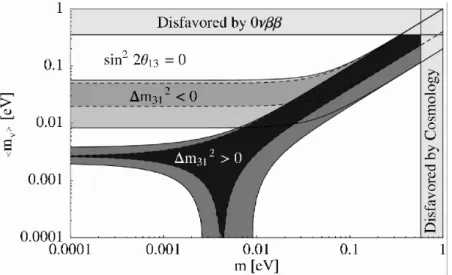
In case of an observation of 0νββ-decay the effective Majorana neutrino mass can be related to the lightest neutrino mass, depending on the neutrino mass hierarchy. Fig- ure 2.6 shows the effective Majorana neutrino mass as a function of the lightest neutrino mass. The two outer bands represent the best fit and 3σ-uncertainties of the oscillation parameters used for the two possible hierarchies. The light band represents the inverted and the dark band the normal hierarchy [53, 54]. As noted previously, cancellations due toCP-violating phases can result in small effective masses for the normal hierarchy.
Nuclear matrix elements The nuclear matrix elements in Equations (2.13) and (2.14) are calculable in at least two different approaches: the Nuclear Shell Model (see e.g., [55, 56]) and the Quasi Random Phase Approximation (QRPA) (see e.g., [57, 58]). The calcula- tions of the M0ν elements are calibrated using the measured 2νββ-rates. In the QRPA approach nuclear model parameters, in particular the particle-particle strength parameter, gpp, can be fixed with this additional information. Calculations are available for several isotopes. For a single isotope the spread between different calculations is of the order of 30%. TheM0ν matrix elements calculated in the QRPA approach are listed in Table 2.2 in the next section.
2.4.2 Experimental considerations
As 0νββ-decay is predicted to be an extremely rare process, it is limited in sensitivity by signal statistics and by the amount of observed background. The following considerations enter into the design of a double beta-decay experiment:
• A good energy resolution to distinguish 2νββ-decays from 0νββ-decays kinemati- cally.
• The rate of 0νββ-decay scales withQ5. An isotope with a highQ-value is therefore expected to have a shorter half-life (Note that the rate of 2νββ-decay scales with Q11). Most double beta-decay experiments use isotopes with aQ-value larger than 2 MeV.
• The amount of background in the region of interest around the Q-value has to be sufficiently low. A large Q-value is advantageous due to the decreasing number of possible background contributions from radioactive decays as Q increases.
18 CHAPTER 2. NEUTRINOLESS DOUBLE BETA-DECAY IN THE SM
Figure 2.6: Effective Majorana neutrino mass,hmνi, as a function of the lightest neutrino mass, m. The light band corresponds to the inverted mass hierarchy, the dark band to the normal mass hierarchy. The mixing angle θ13 is assumed to be zero [53, 54]. The inner (outer) bands correspond to calculations without (with) the 3σ-uncertainties on the oscillation parameters.
• A large target mass increases the number of possible decays. The background typ- ically scales with the total mass (integrated over all isotopes), whereas the signal scales only with the double beta-isotope under consideration. A high natural abun- dance or isotopic enrichment will therefore lead to a better signal-to-background ratio.
• The signal efficiency has to be as high as possible.
• The background has to be as low as possible.
In the following, the background index is defined as the number of observed back- ground events per kg (of total mass), per keV of the spectrum in the region of interest, per year and denoted counts/(kg·keV·y). An estimate of the sensitivity of double beta- decay experiments and the influence of the background are discussed in Chapter 4.
The number of observed 0νββ-events, N, is related to the half-life of the process, T1/20νββ. For a measuring time t≪T1/20νββ the half-life can be expressed as
T1/20νββ ≈ln 2·κ·M·ǫsig· NA MA · t
N , (2.16)
where κ is the mass fraction of the isotope under study, M is the total mass and ǫsig is the signal efficiency. NAis Advogadro’s number andMAis the atomic mass of the isotope.
2.4. DOUBLE BETA-DECAY 19 Experiments are carried out to search for double beta-decay of different isotopes. Ta- ble 2.2 presents a selection of isotopes for which the experimentally important Q-value and natural abundances together with today’s best limit on 0νββ-decay are summarized.
Also shown are the measured half-lives for the 2νββ-decay. The claim of a discovery of 0νββ-decay of 76Ge is discussed in the next section.
Table 2.2: Q-value and natural abundance of possible candidates for 0νββ-decay. Also summarized are the current measurements of the 2νββ-decay (average values taken from [59]) and the current best limits on 0νββ-decay. The nuclear matrix elements are taken from [57]. In the case of76Ge enriched material was used.
Isotope Q-value M0ν Nat. ab. κ T1/22νββ T1/20νββ
[keV] [%] [y] [y] (90% C.L.)
76Ge 2 039 2.40±0.07 7.8 (1.5±0.1)·1021 >1.9·1025[60]
82Se 2 995 2.12±0.10 9.2 (1.0±0.1)·1020 >1.0·1023[61]
100Mo 3 034 1.16±0.11 9.6 (7.1±0.4)·1018 >4.6·1023[61]
116Cd 2 809 1.43±0.08 7.5 (3.0±0.2)·1019 >1.7·1023[62]
130Te 2 530 1.47±0.15 34.5 (0.9±0.1)·1021 >1.8·1024[63]
2.4.3 Search for neutrinoless double beta-decay of 76Ge
The germanium isotope76Ge is a possible candidate for 0νββ-decay. It cannot decay into
76As through a single beta-decay but into76Se via double beta-decay (see Figure 2.5). Its Q-value, denotedQββ in the following, is 2 039 keV [64]. Germanium has two advantages compared to other isotopes: (1) it is the purest producible material in crystalline form and therefore has a very low content of intrinsic background sources, and (2) germanium crystals are semiconductors. This allows to use germanium as source and detector simul- taneously. Very high signal efficiencies of above 90% are achievable for large cylindrical detectors. However, isotopic enrichment in 76Ge is considered necessary for germanium double beta-decay experiments, because the natural abundance is only 7.8%.
The two most sensitive germanium double beta-decay experiments were the IGEX [1]
(Canfranc, Spain) and Heidelberg-Moscow [2] (Gran Sasso, Italy) experiments. Both ex- periments used isotopically enriched germanium detectors.
The IGEX experiment ran from 1991 to 2000 with a total exposure of 8.8 kg·years (117 mole·years). The background index encountered was 0.17 counts/(kg·keV·y). A lower limit on the half-life of 0νββ-decay of T1/20νββ > 1.6·1025 y was deduced from the spectrum in the region of interest, depicted in Figure 2.7 (left).
The Heidelberg-Moscow (HdM) experiment ran from 1990 to 2003 with a total expo- sure of 71.1 kg·years and a background index of 0.11 counts/(kg·keV·y). The final energy
20 CHAPTER 2. NEUTRINOLESS DOUBLE BETA-DECAY IN THE SM spectrum is shown in Figure 2.7 (right). Parts of the HdM collaboration interpret the peak atQββ as a result of the decay under study and claim a discovery with 4.2σ significance and a half-life of T1/20νββ = 1.2+0.4−0.2 y [2]. An earlier publication presented a lower limit of T1/20νββ >1.9·1025 y [60].
Figure 2.7: Left: Energy spectrum measured in the IGEX experiment for a total exposure of 8.8 kg·years (117 mole·years) [1]. The open and black histograms correspond to the energy spectrum without and with the application of pulse shape analysis, respectively.
The black curve represents the 90% C.L. upper limit on the number of 0νββ-events. Right:
Energy spectrum measured in the HdM experiment for a total exposure of 71.1 kg·years [2].
The dashed line represents the estimated background level. The black curves represent fits toγ-lines in the vicinity of theQββ-value.
Two experiments to search for 0νββ-decay of76Ge are planned. TheMajoranaexper- iment [65, 66] in the U.S. will operate about 200 kg enriched germanium detectors in con- ventional cryostats and shielding. A massive effort is being devoted to produce ultra-pure materials for the crystal environment. The GERmanium Detector Array, GERDA [3], is currently under construction in the Gran Sasso underground laboratory, Italy. It is described in more detail in Chapter 3.
Chapter 3
The GERDA experiment
The GERmanium Detector Array,GERDA[3], is a new experiment to search for 0νββ- decay of 76Ge. It is currently being installed in the Hall A of the INFN Gran Sasso National Laboratory (LNGS), L’Aquila, Italy. Its main design feature is to operate bare germanium detectors directly in a cryogenic liquid and minimize the amount of high-Z material in their vicinity.
The first objective of the experiment is to verify or reject the recent claim of discovery of 0νββ-decay [2]. In case the discovery is verified, the statistical significance of the obser- vation is expected to be improved. If the claim is rejected, an improved lower limit on the half-life of the 0νββ-process can be set. Emphasis is placed on the reduction of background.
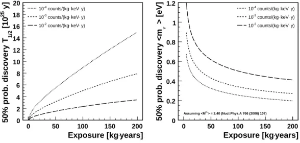
The design goal is to reach a background index of less than 10−3 counts/(kg·keV·y) in the region of interest. This is two orders of magnitude below the background level reached in previous experiments. A lower limit on the half-life of T1/20νββ > 13.5·1025 y can be set with the envisioned total exposure of 100 kg·years1.
The concept of the experiment is based on ideas presented in [67]. The location and technical realization of the project are discussed in the following. This chapter closes with the status of the GERDAexperiment as of Winter 2006/07. Separate chapters on germanium detectors (Chapter 5) and background reduction techniques (Chapter 6) follow and complete the description of the main features of the experiment.
3.1 Concept
Based on the experiences from recent double beta-decay experiments strategies were de- veloped to reduce the background in new experiments. Sources of background are cos- mogenically produced radioactive isotopes in the detectors, muon induced neutrons and electromagnetic showers, and radioactive isotopes in the surrounding of the detectors. The strategies incorporated in the concept ofGERDAare summarized here:
1For a calculation of the sensitivity of GERDA see Chapter 4.
21
22 CHAPTER 3. THEGERDA EXPERIMENT
• Choice of location: cosmic radiation makes low background experiments at sea level impossible due to hadron and muon induced background and cosmogenic activation.
In order to attenuate the flux of cosmic muons and to shield the hadronic component of the cosmic radiation the experiment is located underground.
• Choice of materials: as most of the radioactive background comes from natural decay chains, materials are chosen which have minimal radio-impurities (often levels of the order of µBq/kg are aimed at). Screening experiments are carried out and intercomparisons between different measuring techniques are needed to verify such levels.
• Reduction of material: even with radio-pure materials it is important to reduce the amount of high-Z material close to the detectors. The operation of germanium de- tectors in an ultra-pure cryogenic liquid allows to remove the conventional cryostats.
Instead, especially designed detector suspensions are developed which use a mini- mum of material to support the germanium crystals.
• Shielding: the GERDA design foresees a multi-layer shielding to reduce external radiation. Water as the outermost shell acts as neutron absorber and moderator. A steel cryostat with copper lining shields external γ-radiation. The cryogenic liquid which surrounds the detector array further suppresses external γ-radiation as well as radiation from the cryostat itself.
• Waiting: the half-lives of the cosmogenically produced isotopes 60Co and 68Ge are 5.3 y and 271 d, respectively. Storing the detectors underground and simply waiting will reduce the number of radioactive nuclei.
GERDAwill use enriched high-purity germanium detectors as source and detector si- multaneously. In contrast to previous experiments the detectors are not cooled by a copper cooling finger but are directly inserted into the center of a multi-meter cryogenic buffer.
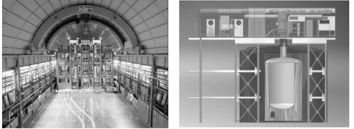
The baseline design foresees liquid argon as buffer. Liquid argon can be produced with a much greater purity than lead or even copper traditionally used for shielding. The cryo- genic liquid will be contained in a copper-lined steel vessel and surrounded by a buffer of ultra-pure water. The 10 m diameter water tank will be instrumented with photo multipli- ers in order to collect Cherenkov light from traversing cosmic muons. The super-structure is mechanically independent of the water tank. A clean room on top of the super-structure houses a lock through which the detectors are inserted into the cryogenic buffer. Plastic scintillator plates on top of the clean room complete the muon veto. Figure 3.1 shows the Hall A of the LNGS before the construction of theGERDA infrastructure (left) and an engineer’s view of the experiment (right).
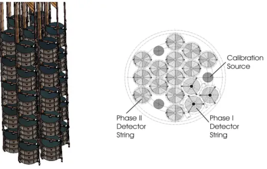
Detectors enriched in the isotope76Ge to a level of about 86% will be deployed as well as reference detectors made out of natural germanium. A phased approached is chosen for the experiment.
3.2. LOCATION OF THE EXPERIMENT - LNGS 23
Figure 3.1: Left: Hall A of the LNGS before the construction of theGERDAinfrastruc- ture. Right: Engineer’s view of the experiment.
In the first phase (Phase I) detectors which were previously operated by the IGEX [1]
and HdM [2] collaborations will be re-deployed. The enriched detectors have a mass of ap- proximately 18 kg in total. For Phase I the envisioned background index is 10−2 counts/(kg·keV·y). The estimated 90% probability lower limit on the half-life of 0νββ-decay, assuming an exposure of about 15 kg·years, is T1/20νββ >2·1025y.
The detectors for the second phase (Phase II) are still under construction. Approx- imately 20 kg of enriched germanium will be used in addition. The background index aimed at is 10−3 counts/(kg·keV·y). An exposure of 100 kg·years is expected resulting in an expected lower limit on the half-life of T1/20νββ > 13.5·1025 y. A 1 000 kg-scale ex- periment is under discussion in cooperation with theMajorana collaboration in a later phase (Phase III).
Novel approaches for the identification and reduction of background events are devel- oped for and discussed in the context ofGERDA. These range from the use of segmented germanium detectors in Phase II [68, 69] to the instrumentation of liquid argon as an active veto against photons [70–72]. An overview of the background reduction techniques developed is given in Section 6.4 after the main sources of background are discussed.
3.2 Location of the experiment - LNGS
TheGERDAexperiment will be located in the Hall A of the INFN Gran Sasso National Laboratory (LNGS), L’Aquila, Italy. It is the worlds largest underground facility for low- background experiments with three halls (each about 100 m times 20 m times 18 m in size). The halls are accessed from a 10 km long freeway tunnel under the Gran Sasso mountains. A large variety of experiments is hosted in the LNGS, most of them focussed on dark matter or neutrino physics.
24 CHAPTER 3. THEGERDA EXPERIMENT The overburden of 1 400 m of rock (corresponding to 3 400 meter of water equivalent, m.w.e.) reduces the external muon flux induced by cosmic rays by a factor of one million compared to the surface. The neutron flux is reduced by a factor of one thousand com- pared to the surface. The content of uranium and thorium in the rock is low. The flux of muons and the activity of radioactive isotopes in the walls of the tunnel are well known.
The location of GERDA is indicated in Figure 3.2 which shows a floor plan of the LNGS laboratory. It is juxtaposed by the Large Volume Detector (LVD) experiment from the north and restricted by a service tunnel from the south. Parts of the cryogenic system, such as tanks for the cryogenic liquid, will be located in the service tunnel towards the east.
Figure 3.2: Floor plan of the LNGS. The GERDAexperiment will be located in Hall A situated between the LVD experiment and a service tunnel.
3.3 Technical realization
The baseline design for the GERDA experiment as of Winter 2006/07 is presented in the following. Since the experiment is still under construction, parts of the design or construction might undergo a revision. Technical details can be found in [73].
3.3.1 Active detector components
The detector has two active sub-systems, the array of germanium detectors and the muon veto system.
Germanium detectors: The detector array consists of hexagonally packed detectors with up to 5 layers. Up to 19 detectors can be placed per layer. The horizontal distance between the centers of two detectors is 9 cm. The vertical clearance between two detectors
![Figure 2.1: Energy dependent flux of solar neutrinos predicted by the solar model BS05(OP) [17].](https://thumb-eu.123doks.com/thumbv2/1library_info/4006874.1540922/18.918.206.652.479.810/figure-energy-dependent-solar-neutrinos-predicted-solar-model.webp)
![Figure 2.5: Isobars for A = 76 [52]. The mass of 76 Ge is less than that of 76 As, but larger than that of 76 Se.](https://thumb-eu.123doks.com/thumbv2/1library_info/4006874.1540922/24.918.140.707.239.439/figure-isobars-mass-ge-larger-se.webp)