Instruments of Modern Physics – A Primer to Lasers, Accelerators, Detectors and all that

Instruments of Modern Physics

– A Primer to Lasers, Accelerators, Detectors and all that

Shaukat Khan, TU Dortmund, Summer of 2014

November 12, 2014

Contents

2 Sources of electromagnetic radiation 3

2.1 Overview . . . . 3

2.2 Black-body radiation . . . . 6

2.3 The laser . . . . 7

2.3.1 Overview . . . . 7

2.3.2 Coherence . . . . 13

2.3.3 Laser types and principles . . . . 14

2.3.4 Effects of ultrashort laser pulses . . . . 19

2.3.5 Generation of ultrashort laser pulses: mode-locking . . . . 23

2.3.6 Amplification of ultrashort laser pulses: CPA . . . . 23

2.3.7 Laser laboratory equipment . . . . 24

2.3.8 Instruments for laser diagnostics . . . . 27

2.3.9 Instruments for laser pulse manipulation . . . . 28

2.4 The X-ray tube . . . . 29

2.5 Synchrotron radiation . . . . 31

2.5.1 Introduction . . . . 31

2.5.2 Synchrotron radiation from dipole magnets . . . . 33

2.5.3 Radiation from undulators and wigglers . . . . 34

2.6 Synchrotron radiation sources . . . . 38

2.6.1 The ”generations” of synchrotron light sources . . . . 38

2.6.2 Short radiation pulses from storage rings . . . . 40

2.7 Free-electron lasers . . . . 44

2.7.1 What is a free-electron laser? . . . . 44

2.7.2 Interaction between electrons and radiation . . . . 45

2.7.3 Low-gain free-electron laser . . . . 47

2.7.4 High-gain free-electron laser . . . . 48

2.7.5 SASE and seeded high-gain FELs . . . . 51

Figure 1:

A special feature of Robert Hooke’s microscope (around 1665 [1]) was the fact that it had its own light source. The light from an oil lamp was focused by a globular glass vessel filled with water (as used by shoemakers at that time).

regime wavelength frequency photon energy temperature

radio waves >1 m <300 MHz <1.24µeV <2.9 mK

microwaves 1 m - 1 mm 300 MHz - 300 GHz 1.24µeV - 1.24 meV 2.9 mK - 2.9 K infrared 1 mm - 750 nm 300 GHz - 400 THz 1.24 meV - 1.65 eV 2.9 - 3864 K visible 750 nm - 400 nm 400 THz - 750 THz 1.65 eV - 3.10 eV 3864 - 7244 K ultraviolet 400 nm - 10 nm 750 THz - 3·10¹⁶Hz 3.10 eV - 124 eV 7244 - 2.9·10⁵K X-rays 10 nm - 0.01 nm 3·10¹⁶- 3·10¹⁹Hz 124 eV - 124 keV 2.9·10⁵ - 2.9·10⁸K gamma rays <0.01 nm (0.1 ˚A) >3·10¹⁹Hz >124 keV >2.9·10⁸K

Table 1:

Regimes of electromagnetic radiation with corresponding wavelength, frequency, photon energy, and temperature for maximum black-body emission according to Wien’s law. Not all regions are well- defined, and slightly deviating values may be found elsewhere.

2 Sources of electromagnetic radiation

2.1 Overview

Some objects can be studied thanks to the radiation they emit themselves, such as excited atoms

or stars. In case the objects can be illuminated, scientific observation was made independent of

natural radiation sources. An early example is shown in Fig. 1, a microscope using a lamp rather

than sunlight. Another example is the use of particle beams from accelerators rather than alpha

particles or cosmic rays.

Here are a few words on natural sources of radiation. As for electromagnetic radiation that can be used to illuminate a sample, the only natural sources are the sun and gamma-ray-emitting radioisotopes. Natural sources of particles, as just mentioned, are radioactivity (which revealed the existence of the atomic nucleus [2]) and cosmic rays (which lead to the discovery of the positron [3], the muon [4], and the pion [5]). In addition to that, there is an abundant – but hardly detected – flow of neutrinos from the sun and other extraterrestrial sources. Yet another type of radiation are gravitational waves, presumed to be emitted by accelerated masses (in analogy to electromagnetic radiation emitted by accelerated charges), e.g. due to the centripetal acceleration of binary stars.

In this section, sources of electromagnetic radiation (or photons) will be discussed, followed by sources of particle beams. Sorted by decreasing wavelength λ, increasing frequency ν, and photon energy E

γ

as given in Tab. 1, the regions of the electromagnetic spectrum and their respective sources are

• Radio waves: The sources are radio antennas driven by amplifiers based on electronic circuits, which – having little application as scientific instruments – will not be considered further.

• Microwaves: Here, radio antennas are driven by various types of amplifiers (klystrons, traveling-wave tubes, magnetrons, and solid-state amplifiers). In addition, there is the maser, a device based on stimulated emission.

• Infrared (IR) radiation, subdivided into far infrared (FIR, λ = 1000 - 20 µm), long-/mid- /short-wavelength infrared (20 - 1.4 µm), near infrared (NIR, 1.4 - 0.75 µm): Thermal radiation plays a role throughout the IR regime. More powerful are laser- and accelerator- based sources in the FIR (terahertz) range, free-electron lasers over a wide wavelength range, and conventional lasers at smaller wavelengths.

• Visible light: Here, thermal radiation is still important (e.g. sunlight or the electric bulb).

There are also various lamps, light-emitting diodes, and many different types of laser.

• Ultraviolet (UV) radiation, below 200 nm Vacuum UV (VUV), below 124 nm Extreme UV (EUV): Apart from some UV-emitting lamps, this is the regime of laser harmonics, synchrotron radiation, and free-electron lasers.

• X-rays: Synchrotron radiation sources cover much of the X-ray regime, free-electron lasers have reached a wavelength of 1 ˚ A, and there is – of course – the X-ray tube.

• Gamma rays: High-energy photons emerge from nuclear reactions, but can also be pro-

duced from particle beams impinging upon a target or boosting photons by Compton

scattering.

By tradition, the sources of electromagnetic radiation fall into two categories:

• Emission described by quantum mechanics, where an excited object (atom, molecule, or atomic nucleus) changes its state and releases energy by the emission of photons. This is true for thermal radiation, lamps, LEDs, laser and gamma sources, as well as characteristic radiation from X-ray tubes.

• Emission due to acceleration of charges, which can be described conveniently and with high accuracy by classical electrodynamics. This is the case for radio- and microwave transmitters, synchrotron radiation, free-electron lasers, and bremsstrahlung from X-ray tubes.

As said above, radio transmitters based on conventional electronics (transistors, integrated circuits) will not be considered further. We will, however, come back briefly to microwave- amplifying devices (such as the klystron) in the context of particle accelerators, in which they provide the accelerating RF waves.

Another class of light sources that will be mentioned only in passing are gas-discharge tubes.

They consist essentially of a vessel containing a gas (or a vapor) with two electrodes. What happens when applying a voltage to those electrodes depends on the voltage value (up to, say, 1000 V) and on the gas pressure (often around a few hPa). There is a number of operation regimes exhibiting quite complex behavior. A rough subdivision is:

• Low voltage leading to pulsed current: The flow of ions and electrons is temporarily caused by cosmic radiation or some other means of ionization.

• Higher voltage (typically above 500 V) with constant current: A self-sustained discharge is caused by the release of electrons from ions impinging on the cathode, while these electrons create new ions (Townsend discharge).

• Drop of voltage after passing through the Townsend-discharge regime, but with higher current: The gas is ionized to an extent that it becomes a plasma and conducts a current (glow discharge). There is only low heat and light emission.

• Another drop of voltage after passing through the glow-discharge regime, and with even higher current: The current through the plasma causes heat, which leads to thermionic release of electrons (arc discharge). The light emission is very strong.

The emitted wavelengths depend on the electronic levels of the gas atoms. These are usually noble gases (e.g. neon: red; krypton: blue) or vapors of solids (mercury: blue; sodium: yellow;

sulfur: white). Sources of UV radiation are e.g. mercury- and deuterium-filled tubes.

Usually, the avalanche growth of the discharge is held at bay by active control of the current.

Some tubes, however, are used as fast switches for high currents (e.g. the so-called thyratron)

by allowing the avalanche to build up, which is particularly fast in hydrogen-filled tubes.

If starting from a glow discharge and reducing the gas pressure, the discharge diminishes but the walls of the vessel start to glow due to fluorescence. It was noticed that an object in the tube (traditionally a Maltese cross) casts a shadow, the position of which is influenced by electric or magnetic fields. In the 19th century, this kind of radiation coming from the negative electrode was termed ”negative light” or cathode rays [6] and turned out to be electrons [7].

2.2 Black-body radiation

Each object emits electromagnetic radiation with a spectrum and intensity depending on its temperature T and emissivity ε. A ”black” body is an ideal emitter with ε = 1, which can be approximated by a small hole in an oven. With setups like this, black-body radiation was extensively studied towards the end of the 19th century, and commercially available instruments for metrology purposes today are still designed that way.

The Stefan-Boltzmann law and Wien’s law connect the temperature to the power per surface area P/A and the wavelength λ

max

of maximum spectral intensity,

P/A = 5.67 · 10

⁻⁸

W

m

²

K

⁴

T

⁴

and λ

max

= 2898 µm K 1

T . (1)

The spectral distribution of black-body radiation was one of the ”19th-century clouds” (as Lord Kelvin put it; the other was the failure to detect the light-conducting ”ether”), and this cloud dissolved when M. Planck reluctantly postulated radiation to come in energy quanta E = hν with h = 6.626 · 10

⁻³⁴

J s = 4.136 · 10

⁻¹⁵

eV s and ν = λ/c being the radiation frequency [8]. The spectral energy density (energy per volume and interval dν) is then

ρ(ν, T )dν = 8π c

³

hν

³

dν

exp(hν/kT ) − 1 , (2)

where k = 1, 381 · 10

⁻²³

J/K is Boltzmann’s constant. A later, somewhat more intuitive derivation of this formula by A. Einstein [9] will ultimately lead us to the laser, since it requires a process called stimulated emission.

Consider a two-level system, e.g. a pile of atoms, with energy difference hν between the levels, N

1

atoms in the lower state 1, and N

2

atoms in the upper state 2 (see Fig. 3 a). Given by statistical mechanics, the ratio N

₂

/N

₁

= exp(−hν/kT ) (known as Boltzmann factor) depends on temperature. The lower the temperature, the more the atoms tend to be in the lower state.

Einstein assumed that atoms can change their state by three processes:

• 1 → 2 by absorption of a light quantum (photon) flying by,

• 2 → 1 by spontaneous emission of a photon,

• 2 → 1 by stimulated emission in the presence of another photon.

Let the probability of spontaneous emission be A

21

or simply A, and the probability of absorption and stimulated emission be equal B

₁₂

= B

₂₁

= B for a given intensity I of the surrounding light field. By tradition, A and B are known as Einstein coefficients. By the way, it is noteworthy that the stimulated emission, newly postulated by Einstein, is actually more ”natural” than the spontaneous emission, because nothing really explains why an atom should decide by itself to jump from state 2 to 1. The debate over this tends towards vacuum fluctuations being the hidden cause of spontaneous emission.

In an equilibrium situation, the number of atoms in either state is preserved by

B I N

1

= B I N

2

+ A N

2

→ B I exp(hν/kT ) = B I + A. (3) Inserting the inverse Boltzmann factor for N

1

/N

2

, and solving for the intensity yields

I = A B

1

exp(hν/kT ) − 1 or ρ(ν, T )dν = 8π c

³

hν

³

dν

exp(hν/kT ) − 1 . (4) Planck’s law is recovered by identifying A/B with the number of radiation modes 8πν

²

dν/c

³

times the energy per mode hν from Planck’s theory (the derivation is found in many textbooks, e.g. [10]).

Apart from initiating quantum mechanics, black-body radiation plays a role in radiation metrology and is omnipresent when doing measurements in the FIR range. It is also fascinating that the cosmic microwave background, believed to be emitted some 380.000 years after the ”big bang” fulfills Planck’s law for T = 2.725 K almost perfectly (within 200 µK) – see [11] for the latest spectacular results on this topic.

2.3 The laser

Among the radiation sources used in modern physics, the laser plays a very prominent role.

Figure 2 shows three examples of different size (sub-mm to 100 m) and output power (µW to PW). Following a microwave source called maser in 1953 [12], the first laser was created in 1960 by T. H. Maiman at Hughes Research Labs in Malibu, CA/USA [13]. Laser

¹

is an acronym for

”light amplification by stimulated emission of radiation”. So, the idea is to amplify light (but there is more to it, e.g. monochromaticity and being diffraction-limited). There are quite a few excellent books on laser physics, e.g. [14, 15].

2.3.1 Overview

Suppose, light travels through a medium along the z axis. If N

₁

and N

₂

are the numbers of atoms in the respective state as before, and a and b are parameters proportional to the Einstein coefficients A and B , the number of photons n changes along the path according to

1If you ever invent something and want it to be a success, make sure that its name rolls off the tongue easily.

Figure 2:

Three rather different lasers – a small tunable diode laser (left, Wikipedia/NASA), a typical Ti:Sapphire laser system (center, DELTA/TU Dortmund), and an array of Nd:glass lasers of the National Ignition Facility at the LLNL in Livermore, CA/USA (right, Wikipedia/NIF).

dn

dz = −b n N

₁

+ b n N

₂

+ a N

₂

. (5) Disregarding the constant spontaneous-emission term for simplicity, the equation and its exponential solution are

dn

dz = b n (N

2

− N

1

) and n(z) = n(0) e

^b(N2−N1)z

. (6) For N

₂

< N

₁

, the solution is just the Lambert-Beer law of absorption with b (N

₁

− N

₂

) = α being the absorption coefficient. For N

2

= N

1

, the number of photons would not change. For N

2

> N

1

, however, the number of photons increases exponentially along the path as e

^{g z}

with b (N

₂

− N

₁

) = g being the so-called gain.

A situation with N

2

> N

1

is called an ”inversion” because it is inverse to the occupation of states described by the Boltzmann factor, where the occupation of the two states approaches equality for T → ∞, but N

₂

never exceeds N

₁

. Thus, an inversion cannot be obtained in a two-level system.

Next, consider a three-level system (see Fig. 3 b) and the rate equations

N ˙

3

= b

p

N

1

− b

32

N

3

− b

31

N

3

and N ˙

2

= b

32

N

3

− b

21

N

2

, (7) where b

ij

is the probability for a transition i → j and b

p

(which could have been written b

13

) describes the probability of ”pumping” the upper state. In the case of equilibrium, the rates ˙ N

3

and ˙ N

₂

must be zero, resulting in N

₃

= b

_p

b

31

+ b

32

N

₁

(for ˙ N

₃

= 0) and N

₃

= b

₂₁

b

32

N

₂

(for ˙ N

₂

= 0). (8)

Equating these two expressions for N

3

and solving for N

2

/N

1

yields

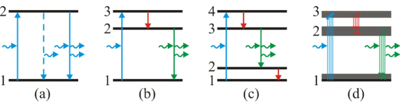
Figure 3:

Sketch of atomic levels with absorption, spontaneous emission (dashed) and stimulated emis- sion of photons (wiggly arrows), (a) a two-level system, (b) a three-level system, (c) a four-level system, (d) a cartoon of a band structure instead of three levels.

Figure 4:

Generic design of a laser with the lasing gain medium, pumped by some energy source (green) and surrounded by an optical cavity comprising two mirrors, one of them slightly permeable or with a hole to release the beam (red). The front and back of the gain medium or its enclosure is often tilted by Brewster’s angle in order to minimize reflection of the polarized laser light. Instead of being confined between two mirror, the cavity may be arranged as a ring (right).

N

2

N

₁

= b

p

b

32

b

₂₁

(b

₃₁

+ b

₃₂

) = b

p

b

₂₁

1

1 + b

₃₁

/b

₃₂

≈ b

p

b

₂₁

1 − b

31

b

₃₂

. (9)

The last step assumes that the transition 3 → 2 is much more likely than the direct decay 3 → 1 to the ground level. The main point, however, is that the ratio N

₂

/N

₁

can exceed 1 if the probability b

21

is small enough. Here comes the inversion! It occurs if state 2 has a long enough lifetime because the transition 2 → 1 is suppressed or ”forbidden” by some selection rule. Many materials can be found in which this is indeed the case, although usually there are four levels rather than three (see Fig. 3 c) and often ”bands” with a broad distribution of states rather than singular levels (see Fig. 3 d). The latter case leads to a broad-band emission spectrum, which – given a fixed product of spectral width and pulse duration by Heisenberg’s uncertainty relation – is a prerequisite for the generation of ultrashort pulses.

So far, only the steady-state situation was considered at which the occupation of the states

does not change anymore. When starting a laser, however, there is an oscillatory behavior,

which is usually referred to as ”spiking”, i.e. the laser intensity is initially spiky and settles to a

Figure 5:

Sketch of laser spiking, given by a numerical solution of Eqs. 10 and 11. A dimensionless inversion parameter (red) proportional to N approaches 1, while the laser intensity (blue) settles at a non-zero value which is much smaller than the initial spikes. The right figure shows the first spike.

steady-state value after some time. This laser dynamics can be described by the following rate equations:

dN

dt = −b N n − a N + R

p

(10) dn

dt = b N n − γ n. (11)

Here, N is the occupation of the upper of two levels and n is again the photon number. The first term of both equations describes the stimulated-emission rate (proportional to N

₂

≡ N and not to N

2

− N

1

as in Eq. 6 assuming N

2

N

1

). The second term of Eq. 10 is the spontaneous emission rate, and R

_p

is the pump rate which is assumed to be constant. The second term of Eq. 11 describes losses in the optical resonator (see below) due to imperfect mirror reflectivity, outcoupling of the laser beam, diffraction and any other effect.

These are two coupled differential equations with nonlinear terms containing a product of the variables N and n. This makes them somewhat similar to the Lotka-Volterra equations, describing the oscillations of predator and prey populations with a 90

^◦

delay between them (if wolves finished off most of the sheep, the wolf population decreases with a delay due to lack of food, allowing the sheep population to recover, the wolf population follows, and so on).

At the startup of the laser, N first increases almost linearly with time due to the constant

pump rate. After reaching the threshold at which stimulated emission exceeds the losses, N rises further but soon the number of photons rises dramatically and reduces N below the threshold, which quenches further photon emission. This was the first spike, and once N surpasses the threshold again, the second spike occurs, and so on.

Figure 4 shows a generic laser design. While the laser material (the gain medium) is supplied with energy (”pumped”) to keep up the inversion, the radiation field builds up between two mirrors forming an optical cavity (also called resonator). One of the mirrors is slightly permeable or has a small hole to allow a small fraction of the radiation to escape as laser beam. There are several types of gain medium and different ways of pumping. The gain medium can be a

• a neutral or ionized gas,

• a liquid solution,

• a solid insulating or semi-conducting crystal or glass,

• an optical fiber,

• a beam of relativistic electrons.

The way of pumping can be pulsed or continuous, involving

• collisions of atoms/molecules with others or with electrons,

• light from another laser or some sort of lamp,

• a chemical reaction,

• adiabatic expansion of a hot gas,

• the energy contained in an electron beam.

The optical cavity or resonator may

• be between concave, convex or plane mirrors, or between the medium’s surfaces,

• follow a straight axis between two mirrors or folded by additional mirrors,

• follow the curls of an optical fiber,

• be confined between two mirrors or ring-shaped,

• be omitted altogether.

In these listings, the respective last item describes the free-electron laser (FEL). Since FELs are quite different from other lasers (no atomic levels, no external pump, and in some cases no cavity), a separate section will be devoted to them.

Whatever the design of the optical cavity, the length L along a certain axis plays a particular role and the gain medium often has a cylindrical shape aligned to that axis. While the light is allowed to escape through the transverse boundaries of the medium, a standing wave with wavelength λ builds up along the cavity axis under the condition of nodes of the electric field at either end, i.e. L is equal to λ/2 times a large integer q. Along a frequency scale ν, so-called modes labeled by q form a comb with

ν

_q

= v λ = qv

2L , (12)

where v is the velocity of light, which is lower than c in the gain medium. For v ≈ c and a cavity with L = 1 m, the distance between adjacent modes would be c/2L ≈ 150 MHz.

Out of this frequency comb, a number of lines lie within the bandwidth of the lasing atomic transition. If a single mode is desired, the bandwidth should be small and the line spacing should be wide, corresponding to a short cavity. Further mode selection can be done by inserting some wavelength-filtering device into the cavity, e.g. a prism that deflects different wavelengths into different directions, a pair of parallel surfaces (Fabry-Perot interferometer, also known as

”etalon”) at a distance matching an integer multiple of λ/2, or a grating replacing one of the end mirrors.

Between two arbitrary spots on either end mirror of the cavity, there is a variation of the length L. This variation may be small, but so is the wavelength of near-visible light, and the non-integer ratio of L and λ/2 gives rise to transverse modes. These modes are labeled TEM

_mnq

or just TEM

mn

(omitting the longitudinal mode index), where TEM indicated transverse electric and magnetic fields and m, n are the numbers of nodes (zero field) in two transverse directions:

horizontal and vertical for rectangular modes or radial and angular for cylindrical modes. The most common and usually desired mode is TEM

00

, which yields a Gaussian beam shape with small divergence, is easiest to focus, and has no transverse phase shift.

Another important property of the optical cavity is the amount of losses, expressed either by a coefficient γ as above or by the Q value (quality factor, commonly used in microwave theory) given by Ω/γ, where Ω = 2πν

1

is the eigenfrequency of the resonator. Lasing requires γ to be small and Q to be large. Since starting the laser can produce spikes with a peak power much larger than the equilibrium value, the Q value is sometimes deliberately reduced and then suddenly switched to a high value in order to produce a powerful pulse. Technical issues of

”Q-switching” will be described later.

Before discussing various laser types, a rather striking feature of laser light shall be addressed.

Figure 6:

Speckle pattern from a laser pointer (left, from Wikipedia, author Deglr6328) and in a sonographic image (right, adapted from Wikipedia, author Aoineko).

2.3.2 Coherence

When laser light illuminates a surface in a uniform way, a fine granular pattern is observed which became known as ”speckle”. This pattern is never observed with sunlight or light from a lamp, but it is also found e.g. in ultrasound images of the human body or in radar images.

The speckle pattern is caused by the wavelength-scale random roughness of the reflecting object, and is washed out in the case of light lacking a quality called ”coherence”. Laser light is said to be ”coherent” (which is also true for radar and ultrasound waves), light from an electric bulb is called ”incoherent”, although this is a gross simplification.

Temporal (longitudinal) and spatial (transverse) coherence measures to what extent phases within a field of waves (such as light) at different points of time or space, respectively, are related.

This way, it predicts to what degree an interferometric experiment would work. Standard examples are the Michelson interferometer for longitudinal coherence and Young’s double-slit experiment for the transverse case. Coherence is a gradual property (not just present or absent), and the degree of coherence between two given points would be 1 for full coherence and 0 for no coherence at all. Obviously, the separation between these two points is important (if they coincide in space and time, the degree of coherence must be 1). Alternatively, a longitudinal or transverse coherence length can be defined, stating at which distance the coherence drops from 1 to a certain value.

More formally, the correlation functions for the electric field E between two points in space and time is given by

Γ(~ r

1

, ~ r

2

, t, τ ) = 1 T

Z t+T /2

t−T /2

E

^∗

(~ r

1

, t

⁰

) · E(~ r

2

, t

⁰

+ τ ) dt

⁰

≡ hE

^∗

(~ r

1

, t) · E (~ r

2

, t + τ )i. (13)

The normalized correlation function and the coherence is then defined by

γ (~ r

₁

, ~ r

₂

, t, τ ) = Γ(~ r

1

, ~ r

2

, t, τ)

p

Γ(~ r

₁

, ~ r

₁

, t, 0) Γ( r ~

₂

, ~ r

₂

, t, 0) and C(~ r

₁

, ~ r

₂

, t, τ) = |γ(~ r

₁

, ~ r

₂

, t, τ)|. (14) The correlation functions in the denominator at the same position ~ r

i

and time (τ = 0) are just the intensities for i = 1, 2. These expressions are usually found in simplified versions, e.g.

without time t in the case of a stationary light field, and either

• omitting τ to describe the transverse coherence without temporal delay, or

• setting ~ r

₁

= ~ r

₂

= ~ r to describe the longitudinal coherence at a given position.

In either case, the absolute value of the normalized correlation function is the coherence, a real number between 0 and 1, which can be measured by performing a suitable interferometric experiment. In such an experiment, the light intensity forms a fringe pattern due to interference with minima I

min

and maxima I

max

. The degree to which this pattern occurs is expressed by the so-called visibility

v = I

_max

− I

_min

I

_max

+ I

_min

, (15)

and it turns out that this rather intuitive quantity is just equal to the coherence C in typical setups like the Michelson interferometer.

2.3.3 Laser types and principles

Here is a list of lasers which is by far not complete. We can only mention typical representatives of a number of lasers types which you are likely to come across when working in a physics lab.

Laser for ultrashort pulses will be discussed in more detail in a separate section, and free-electron lasers will be treated in the context of synchrotron radiation.

Neutral-atom gas lasers

The most common and well-known neutral-atom gas laser is the helium-neon (He-Ne) laser.

In 1960, a few months after the pulsed ruby laser, it was the first continuous laser

²

, initially operated at a wavelength of 1152 nm (IR) and later at 633 nm (red light). Although now largely replaced by more cost-effective and compact laser diodes (e.g. to scan bar codes at the supermarket check-out), it is still in high demand when high precision is required. Its coherence length can amount to kilometers. A weak point of He-Ne lasers is the output power, which is limited to several 10 mW.

2Continuous operation is also called continuous-wave or CW mode, and sometimes ”free-running” operation.

He-Ne lasers consist of a discharge tube, a capillary less than 1 m in length and 1 mm or less in diameter, protected by a cylindrical tube with a diameter of a few cm. The tube is filled with a 10:1 mixture of He and Ne at a pressure around 10 mbar. A (usually separate) power supply creates a voltage of several kV to maintain a He glow discharge.

The peculiarity of this (and some other) lasers is that the pumped and the lasing atoms are not the same. Among other levels, the He atoms can be excited to 20.6 eV by electron collisions. By He-Ne collisions, the Ne atoms are excited to a metastable level (5s) at a similar energy. Stimulated emission leads to a level at 18.7 eV (3p), from which the Ne atoms return to the ground state by spontaneous emission and collisions with the capillary wall. The power is limited by the Ne density and the capillary length, both of which cannot be arbitrarily increased for a number of reasons.

Other neutral-atom gas lasers involve metal vapor, such as the continuous or pulsed helium- cadmium laser at 325 nm (UV) and 442 nm (blue) with output powers around 100 mW, or the pulsed copper-vapor laser at 511 nm (green) and 578 nm (yellow) with average powers up to the kW regime. This and the gold-vapor laser are necessarily pulsed because of the relatively long lifetime of the lower laser level, which makes them ”self-terminating”.

In contrast to the He-Ne laser, many gas lasers consume their lasing material due to chemical reactions or implantation into the walls, and their fill has to be replenished from a reservoir.

Ion lasers

Some gas lasers use ionized atoms, such as the argon (Ar

⁺

) laser operating in CW mode at many wavelengths, exceeding output powers of several 10 W in the UV regime (334 - 364 nm) as well as between 488 nm (blue) and 515 nm (green). Due to a discharge current and high plasma temperature, elaborate cooling is required. Only about 0.1 % of the wall-plug power goes into the laser beam, most of which must be removed by water cooling. Despite their low power conversion efficiency, they still play an important role as high-power sources in the blue and UV regime.

Another ion laser with similar properties and wavelengths ranging from 407 nm (blue) to 676 nm (red) is the krypton (Kr

⁺

) laser.

Molecular gas lasers

In addition to atomic transitions, molecules offer a large variety of transitions between vibra- tional and rotational states, mostly in the IR regime.

The carbon dioxide (CO

₂

) laser, invented in 1964, offers continuous operation with multi-kW

power and high conversion efficiency (up to 20 %) and is applied in industry for cutting and

welding metal. The most important transitions are between vibrational states around 0.3 eV

and states between 0.17 and 0.18 eV forming bands due to additional rotational levels, resulting

in many narrow-bandwidth transitions at wavelengths between 9.3 and 10.7 µm (IR). The upper

levels can be pumped directly, but mixing CO

2

with N

2

and pumping metastable nitrogen levels is more efficient. In addition, helium is added to improve the thermal conductivity of the gas and reduce the unwanted population of low CO

₂

levels. The CO

₂

molecules return to their ground state by spontaneous emission and collisions with helium. In contrast to the He-Ne laser, collisions with the tube wall are not required, which allows to make the tube much larger.

For cooling and due to chemical reactions, the CO

₂

gas is usually pumped in various ways:

either along the laser axis or transversely, slow or fast flow. There are also different ways of maintaining the discharge, either by a high voltage or by an RF wave.

Another important class of molecular gas lasers are excimer lasers invented in 1970. ”Ex- cimer” means excited dimer and refers to molecules that are formed by two atoms and exist only in an excited state following an electric discharge. Since the ground state does not exist, such excited states always constitute an inversion. The importance of excimer lasers lies in the fact that transitions between excimer and unbound state are in the UV regime. The molecules consist of two noble gas atoms (Ar

2

, Kr

2

, Xe

2

) or a noble gas and a halogen element (Cl or F), wavelengths range from 126 nm (Ar

₂

) to 351 nm (XeF) with output powers around 100 W. The lifetime of the excited dimer (typically 10 ns) determines the laser pulse duration with repetition rates in the kHz range.

Another molecular gas laser is the nitrogen (N

₂

) laser at 337 nm with an output power around 100 W. Lasing takes place between very short-lived vibrational levels of the N

2

molecule. Due to their short lifetime and self-terminating nature, there is little build-up of the light within a cavity, and there is usually just one mirror (operation without mirrors is sometimes called

”super-luminescence” or ”super-radiance”). As a fun project, even air at normal atmospheric pressure can be used for lasing [15, 16].

Dye lasers

Dyes are colorful organic substances with a multitude of molecular transitions over an ex- tended range. In 1966, it was discovered that they can be used for lasing, and placing a dispersive element in the cavity the output wavelength can be tuned. Dye lasers are pulsed or continuous and cover the range of 550-630 nm (green to red) with output powers of several W.

The most prominent example of a dye is rhodamine 6G, lasing around 580 nm. To avoid decomposition under the influence of light, the dye is circulated. It is either solved in alcohol which is made to form a liquid jet from a nozzle, or in another solvent like glycol which flows through a cuvette (a vessel with parallel transparent walls). Dye lasers can be pumped by flash lamps or, more often, by other lasers such as argon or frequency-doubled Nd:YAG lasers (see next).

Solid-state lasers

Instead of forming a gas or being solved in a liquid, the lasing atoms may also be embedded

in a transparent host material. The host material provides thermal conductivity, it influences to a certain extent the levels of the lasing atoms, and – what is most important – their density is much larger than in a gas. The density ratio of active atoms (or ions) to host atoms is usually limited to 0.01 or so, but may be up to 0.25 in particular cases.

Host materials should have good optical quality and should comprise atoms that are easily replaced by chemically similar active atoms. This is particularly the case for yttrium, being part of yttrium garnet (abbreviated ”YAG”, Y

3

Al

5

O

12

), yttrium lithium fluoride (”YLF”, LiYF

4

) and yttrium orthovandanate (”YVO”, YVO

₄

), which can be replaced by rare-earth ions (like Nd, Er, Yb) or the transition metal Cr. Other examples are sapphire (Al

₂

O

₃

), which readily accepts impurities of Ti or Cr, and glass (SiO

2

) doped with Nd ions.

Standard examples are continuous or pulsed neodymium-doped lasers (in the usual notation Nd:YAG, Nd:YLF, or Nd:YVO) invented in 1964. Here, the Nd ion retains its properties such that, whatever the host material, it constitutes a 4-level system with a favored pumping wave- length of 808 nm and a lasing transition at 1064 nm. Output powers in the 10 kW range are possible, and for many applications, the laser light is frequency-doubled in a non-linear crystal (see below), resulting in a bright laser beam at 532 nm (green).

Nd lasers have profited very much from the development of powerful laser diodes. Initially, pulsed Nd lasers were (and some still are) pumped by xenon flash lamps, where the laser and the flash lamp rod would sit in the two focal points of an elliptical mirror to maximize the energy transfer. Nowadays, the optical cavity of the Nd laser is often folded by ”dichroic” mirrors.

Dichroic (Greek: two colors) in this context means that the mirrors reflect the Nd laser light while letting the pump wavelength pass. This way, 808 nm radiation from diode lasers (often transported through fiber bundles) can be directed from both sides along the laser axis onto the Nd-doped crystal.

As a side remark: the performance of flash lamps degrades over time, and they have to be replaced every now and then, which is a nuisance but not very expensive. Diode lasers, on the other hand, have superior properties and degrade very little over their lifetime – but once they die (after 10000 hours or so), their replacement can be as expensive as a BMW.

Another important solid-state laser is Ti:sapphire, which has become the workhorse of short- pulse applications. Here, the Ti ions are influenced very much by the host material. Coupling to oscillations of the sapphire lattice results in rather broad absorption and emission bands.

Usually, Ti:sapphire lasers are pumped by frequency-doubled pulses from a Nd laser at 532 nm and emit radiation around 700 to 900 nm (near-IR). Due to the large emission bandwidth, their pulses can be as short as 10 fs. Much effort went into the design of Ti:sapphire amplifiers, resulting in average powers of several W – which does not sound too impressive – but with pulse energies exceeding 10 J within a few 10 fs, reaching peak powers in the PW (10

¹⁵

W) regime.

More on these fascinating laser systems will be said below in the section devoted to ultrashort

laser pulses.

Fiber lasers

Even more than science, telecommunication technology has profited from the advent of fiber lasers. It was noted early on (already in 1961) that a suitably-doped optical waveguide might be a good gain medium because of its length. Fiber lasers are solid-state lasers with some glass as host material doped by rare-earth atoms, most commonly erbium (wavelength 1.55 µm), but also ytterbium (1.03 µm) or neodymium (1.06 µm).

Fiber lasers are pumped by diode lasers around 800-940 nm, which are readily available, and ways have been found to efficiently couple their light into the fiber. Output powers have reached the kW regime. For scientific applications, fiber lasers with short pulse duration are of interest.

Devices with pulses below 100 fs are now commercially available. We will return to fiber lasers as precise clocks in the context of particle accelerators.

Laser diodes

Diodes are elements with an interface between p- and n-doped semiconductors (p-n junction).

A semiconductor has a smaller gap between valence band and conduction band than an insulator.

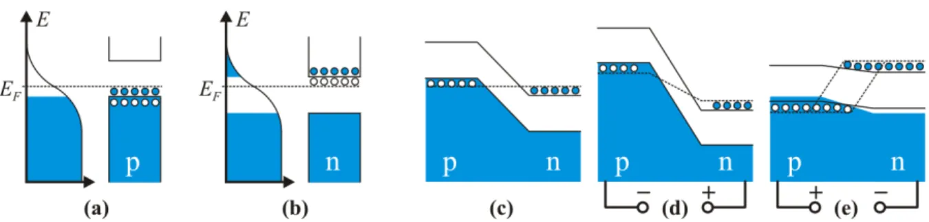
A p-doped material has impurities that are likely to be filled by electrons from the valence band, leaving a ”hole”. An n-doped material has impurities with an excess of electrons which easily fill the conduction band. Putting p- and n-doped material in close contact results in recombination of electrons and holes near the interface, leaving a zone that is depleted of charge carriers, electrons as well as holes. Applying a reverse bias (positive at the n-doped part of the diode) increases the depleted area. A forward bias (positive at the p-doped part) pulls electrons towards the p-doped side and holes in opposite direction, thus allowing a current to flow and electrons can combine with holes under the emission of light. As illustrated by Fig. 7, the electrons are at a higher energy level than the holes, and the continuous replenishment of electrons by the currents maintains an inversion.

Laser diodes are made from various semiconducting materials, e.g. several compounds of Ga, As, In, and P (emitting red or IR light) or GaN (the famous blue laser diode), but notably not Si. Silicon happens to be a so-called ”indirect” semiconductor. This means that the maximum of the valence band and the minimum of the conduction band are separated by a rather different wavevector ~ k with an absolute value of the order of the inverse lattice constant. The wavenumber of a photon, on the other hand, is of the order of the inverse wavelength. This mismatch means that the momentum of a photon is far too small to fulfill momentum conservation in transitions across the Si gap (these transitions are mediated by phonons, the quanta of lattice vibrations).

While lasing of a diode was demonstrated as early as 1962, lasing at room temperature

requires another trick, proposed in 1963 but achieved seven years later: a ”heterostructure” of

two materials suppresses losses by confining the lasing process to a small region and acts also as

a waveguide. The optical cavity is provided by the coated faces of the lasing crystal. A sub-mm

laser diode is usually mounted together with a monitor photodiode in a cylindrical housing and

Figure 7:

Level schemes of a p-doped semiconductor (a) with holes in the valence band and an n-doped semiconductor (b) with electrons in the conduction band. Also sketched is the electron density as function of energyE with EF being the Fermi edge. Putting p- and n-doped material in close contact to form a diode (c) causes a zone depleted of charge carriers. A reverse bias widens this zone (d), a forward bias reduces it (e) and allows a current to flow causing a continuous supply of electrons in an upper level, i.e.

an inversion.

protected by a glass window. The monitor diode picks up some of the emitted light and is used to control the current through the laser diode.

For high-power applications in the kW range, many laser diodes are combined. Several laser diode strips can be arranged on the same substrate in a lithographic process. A ”diode laser”

consists of several such laser diode ”bars” together with a heat sink and some optical elements for focusing and wavelength selection.

2.3.4 Effects of ultrashort laser pulses

The meaning of ”ultrashort” has changed over time and today refers to the femtosecond regime, while attosecond physics is already emerging.

Consider an atom in a solid-state lattice oscillating with frequency ω. Equating the oscillation energy E = ¯ h ω with the thermal energy k T , where k is Boltzmann’s constant and T = 300 K is the ambient temperature, yields an oscillation period of τ = 2π/ω = 160 fs. Now consider an electron with angular momentum 1¯ h in Bohr’s classical model of the hydrogen atom. The orbit radius is then r = 5.3 · 10

⁻¹¹

m, the velocity is v = 2.2 · 10

⁶

m/s, and the resulting revolution period is 2πr/v = 150 as. These admittedly handwaving arguments suggest that the motion of atoms takes place on the femtosecond scale, while phenomena within atoms occur in the attosecond regime.

Short laser pulses can have a half-width duration of a few 10 fs or, with some tricks, even shorter. The workhorse in this field is the Ti:sapphire laser with a wavelength around 800 nm, corresponding to a period length of 2.7 fs, which limits the possible pulse duration. Pulses below 100 fs have been achieved with other solid-state, fiber or dye lasers, and finding new suitable materials is an active field of research.

In addition to being sensitive to fast phenomena in matter, new classes of effects emerge

when short pulses pass through matter:

• The pulse duration is related to the spectral width by the uncertainty relation σ

t

· σ

E

≥

¯

h/2 (using rms values). Thus, short pulses have a broad spectrum and are affected by dispersion, i.e. the dependence of the index of refraction on the wavelength. This effect is independent of the pulse intensity.

• For a given pulse energy, short duration implies high peak power causing intensity-dependent effects. A lot of seemingly self-evident facts in optics – the superposition principle, a con- stant index of refraction for a given wavelength, etc. – are only true if the dielectric polarization of the medium is linearly proportional to the impinging electric field, which no longer holds for ultrashort laser pulses.

In the following, these effect will be briefly addressed, starting with the consequences of large bandwidth. Using half-maximum widths of pulse duration and frequency the uncertainty relation reads

∆t · ∆ν ≥ 0.441 (16)

for Gaussian pulses. The number 0.441 is equal to 2 ln 2/π and its value would be different for other pulse shapes (e.g. 0.142 for Lorentzian pulses). In any case, there is a minimum value for this so-called time-bandwidth product, and a light pulse that meets this limit is called a Fourier-limited pulse.

The following is discussed in more detail in e.g. [14, 15, 17, 18, 19]. The nomenclature used here is close to [14], which we find particularly clear. Let the electric field of a Gaussian laser pulse be

E(t) = E

₀

exp(−at

²

) exp(iω

₀

t + ibt

²

) = E

₀

exp(−at

²

) exp(iφ) = E

₀

exp(−Γt

²

) exp(iω

₀

t) (17) with φ ≡ ω

0

t + bt

²

and Γ ≡ a − ib. The ”instantaneous” intensity along the pulse can be defined as

I(t) = |E (t)|

²

= E

₀²

exp(−2at

²

). (18) Note that the width parameter a is related to the standard deviation σ

t

=

^p

1/(4a) and the full-width half maximum ∆t =

^p

2 ln 2/a, both referring to the intensity distribution (not the electric field). The parameter b introduces a so-called ”chirp”, a variation of the ”instantaneous”

frequency along the pulse. This frequency (which tells how fast the phase changes with time) is the time-derivative of the phase

ω(t) = dφ(t)

dt = ω

₀

+ 2bt. (19)

It can be shown (and here we leave out all tedious details) that the frequency width of the spectrum increases by introducing a chirp, and so does the time-bandwidth product:

∆ν =

√ 2 ln 2

π

√ a

q

1 + (b/a)

²

and ∆t · ∆ν = 0.441

q

1 + (b/a)

²

. (20) It is important to emphasize that the chirp was introduced while keeping the pulse duration

∆t constant. What, if we keep the frequency width constant? The answer starts from the frequency-domain description of a pulse which is propagated along a distance z

E(ω, z) = ˜ E

₀

exp

[ω − ω

₀

]

²

/4Γ

₀

exp(−ikz), (21) where the pulse starts at z = 0 with Γ

₀

≡ a

₀

(no initial chirp) and evolves under the influence of dispersion, i.e. the frequency-dependence of refractive index n(ω) and wavenumber k(ω) = 2πn(ω)/λ. In most transparent media, these functions rise towards shorter wavelengths due to resonances in the UV region (as described by the Drude-Lorentz oscillator model). Given the large bandwidth of short pulses, at least three terms of the Taylor expansion should be considered

k(ω) = k(ω

₀

) + k

⁰

(ω

₀

) · (ω − ω

₀

) + 1

2 k

⁰⁰

(ω

₀

) · (ω − ω

₀

)

²

+ . . . (22) It is well-known that v

_p

= ω

₀

/k(ω

₀

) is the phase velocity, v

_g

= dω/dk = 1/k

⁰

(ω

₀

) is the group velocity, and the two are not equal in the case of dispersion. As the pulse propagates, the phase of the electromagnetic field will thus move within its Gaussian envelope. The third term, the curvature of k(ω), gives rise to a frequency-dependent group velocity which (again leaving out tedious details) causes the pulse length to change according to

∆t =

√ 2 ln 2

√ a

q

1 + (b/a)

²

and ∆t · ∆ν = 0.441

q

1 + (b/a)

²

, (23) with the approximate parameters a ≈ a

0

and b(z) ≈ 2a

²₀

k

⁰⁰

z. In this context, k

⁰⁰

is called

”group velocity dispersion” (GVD). If a Fourier-limited pulse is sent through glass, as an exam- ple, the pulse becomes chirped and increases in length by a factor

^p

1 + (b/a)

²

=

^p

1 + (z/z

_D

)

²

, where z

D

= (2ak

⁰⁰

)

⁻¹

is the dispersion length, at which (in analogy to the Rayleigh length) the pulse duration is increased by √

2. Sometimes, laser pulses are sent through a glass block to deliberately create a chirp. In other cases, the transition through matter (lenses, windows etc.) is ”pre-compensated” by starting with a negatively chirped pulse which becomes shorter when passing through the right amount of matter.

As mentioned before, short pulse duration implies high peak power, reaching nowadays 1

PW to study exotic states of matter (e.g. plasmas with relativistic electrons and ions), while

the most common Ti:sapphire lasers are in the 100 GW range. The polarization P ~ of a material

under the influence of a light pulse is to first order proportional to the electric field E, but as ~

the light intensity increases, higher orders cannot be ignored. Here, the discussion is restricted to isotropic media, where P|| ~ E. The scalar value of the polarization is then ~

P = ε

0

χ

⁽¹⁾

E + ε

0

χ

⁽²⁾

E

²

+ ε

0

χ

⁽³⁾

E

³

+ . . . (24) The proportionality constant χ

⁽¹⁾

is known as susceptibility in linear optics, but now there is a second-order and even third-order susceptibility to be considered. In non-isotropic media, e.g. birefringent crystals, the polarization and field must be written as vectors and the higher- order susceptibilities are tensors. Inspection of the simplified case of Eq. 17 already reveals two non-linear phenomena.

• The second term involves the square of a sinusoidal electric field, which results in a po- larization at the doubled frequency, as the identity sin

²

x = (1 − cos 2x) /2 shows. Thus,

”blue” (400 nm) light can be created by sending a ”red” (800 nm) laser pulse

³

into a material with suitable χ

⁽²⁾

. This process is known as second-harmonic generation (SHG), and a popular material for this purpose is ”LBO”, lithium triborate LiB

3

O

5

.

• The third term multiplies the sinusoidal electric field with the square of the field, i.e.

the light intensity. With similar reasoning as above, the presence of a frequency-tripled component can be shown. More interesting is the fact, that the square of the electric field times χ

⁽³⁾

can be understood as an intensity-dependent susceptibility, leading to an index of refraction that depends on intensity, usually written as n(I ) = n

0

+ n

2

I (or n

2

/2 in some books), where n

₂

(in m

²

/W) is sometimes called Kerr coefficient. For laser pulses, the central part with highest intensity is therefore slowed down in a medium with n

₂

> 0, causing ”self-focusing” or a ”Kerr-lens” effect.

Yet another effect of high peak power is high-harmonic generation (HHG), which is employed to generate radiation at short wavelengths and is one of the keys to attosecond physics. When a short laser pulse with wavelength λ is sent through a gas, light at odd harmonics (λ

_h

= λ/h with h = 3, 5, 7 . . .) is emitted. The semi-classical Corkum model [20] states that electrons of the gas atoms can tunnel through the Coulomb barrier formed by the Coulomb potential (∼ −1/r) and the potential from the strong electric field of the laser (∼ r), and when the field reverses, the electrons are smashed back into the atom and recombine with violent radiation emission. Due to the oscillating electric field, this happens twice per laser period λ/c. The Fourier transform of a ”comb” (a succession of equidistant spikes) along the time axis is a comb in the frequency domain. Thus, the spectrum of radiation pulses occurring twice per laser period shows odd harmonics of the laser frequency. Typical HHG spectra drop in intensity with increasing h by several orders of magnitude, level off at a so-called plateau of nearly constant intensity, and drop again at some cut-off value h

max

which can exceed 100.

3 Light at 800 nm is not red but in the near IR range. In the usual lab jargon, however, ”red” and ”blue”

generally refers to light of long and short wavelength, respectively.

2.3.5 Generation of ultrashort laser pulses: mode-locking

Short laser pulses on the nanosecond level can be generated by Q-switching. As discussed around Fig. 5, short and intense pulses show up when lasing is initiated, which is done by quickly increasing the quality factor Q of a laser resonator using an optical switch (see Sect.

2.3.9).

The technique to create femtosecond pulses is called mode-locking. Here, many longitudinal resonator modes with frequencies ω

_q

= qπv/L add up, where q is an integer, v is the propagation velocity within the resonator and L is the resonator length (see also Eq. 12). The electric field of a mode q within a Gaussian spectrum of central frequency ω

0

and rms width σ

ω

is

E

q

(t) = E

0

· e

^{−12(ωq−ω0)2/σω2}

· e

^i(ωqt+ϕq)

. (25) Mode-locking refers to a situation in which all phases ϕ

q

have a fixed relationship to each other at all times. Arbitrarily setting ϕ

q

= 0, for example, results in a maximum at time t = 0 due to constructive interference. With typically 10,000s of modes contributing, this condition is not met at slight deviations from t = 0 since the waves with phases ω

q

t with many different frequencies cancel each other, and thus we have a short pulse. However, constructive interference occurs again at fixed time intervals ∆T = 2L/v, and so we have a train of short pulses.

Mode-locking is accomplished by various techniques which will not be discussed here, because a very common method is to do nothing. Self-locking of modes occurs due to the Kerr-lens effect (see last section), which focuses an intense light distribution stronger than a weak one, thus providing positive feedback on the generation of short pulses. The process must be actively initiated by a fast intensity fluctuation, e.g. a quick motion of a mirror or prism within the optical cavity (if fact, self-locking was discovered by jerking the laser table [17]).

Lasers producing ultrashort pulses, e.g. Ti:sapphire lasers at 800 nm wavelength, are called

”oscillators”, as opposed to amplifiers which receive pulses from an oscillator and amplify them.

Such an oscillator consists of a folded cavity of length L = 1-2 m between two mirrors. Frequency- doubled light (532 nm) from a Nd laser is coupled into the cavity through one of the folding mirrors (dielectric mirrors reflect 800 nm laser light and are transparent for other wavelengths) to pump the Ti-doped sapphire crystal with several W of power. In addition, the cavity contains a set of prisms to compensate the group velocity dispersion of the crystal. Typical output powers are several 100 mW. With a pulse separation of the order of ∆T = 10 ns, the pulse energy is several nJ.

2.3.6 Amplification of ultrashort laser pulses: CPA

Ti:sapphire amplifiers, again pumped by frequency-doubled Nd lasers, can increase the energy

of pulses from an oscillator from the nJ to the µJ or mJ level (factor 10

³

to 10

⁶

), depending on

the output repetition rate. The average output power of oscillator and amplifier is usually not

very different (maybe a factor of 10), and a higher pulse energy corresponds to a lower fraction

of amplified pulses. As an example, if the pulse energy is raised from the nJ to mJ level, the repetition rate is reduced from the 100 MHz to the kHz regime. By using optical switches, e.g.

Pockels cells (see below), only every, say, 100,000th oscillator pulse is amplified.

Despite this dramatic reduction in pulse rate, the high peak power of the amplified pulses would destroy the crystal if not another ingenious technique was invented: chirped-pulse ampli- fication (CPA) [21]. Here, the short pulses are stretched by a large factor (1000 or more), then safely amplified, and finally recompressed to their original fs-scale length. The ”stretcher” chirps and thus stretches the pulses (see last section), which is done in some systems by GVD in a piece of glass, but more commonly by gratings creating wavelength-dependent path lengths. Since there is a clear correlation between the longitudinal position along the pulse and the wavelength, the ”compressor” can make the pulse roughly as short as before by inverse wavelength-dependent path lengths (again using gratings).

There are two major design types for CPA amplifiers, in which the pulse pass through the amplifying crystal several (typical 10-15) times to make full use of the inversion:

• Multipass amplifiers: the pulses are sent through the crystal by mirrors under slightly different angles for each path (if the passes were perfectly identical, the pulses would go back into the oscillator after the second pass).

• Regenerative amplifiers: the pulses are injected into an optical cavity by an optical switch (see Sect. 2.3.9), go back and forth several times within the cavity while passing through the crystal, and are then ejected, again using an optical switch.

Regenerative amplifiers are said to be easier to adjust and produce higher overall gain, since the number of passes is under the control of the optical switches. Multipass amplifiers are said to produce shorter pulses because the pulses pass only through the crystal, while the optical switches of the regenerative amplifier constitute additional matter.

2.3.7 Laser laboratory equipment

Laser laboratories have to meet certain demands for the safe and reliable operation of the sophisticated systems they accommodate:

• Clean environment to prevent optical components from accumulating dust. Laser labs range from just a tolerably clean room to an elaborate cleanroom, in which people wear shoe covers, lab coats and hairnets. Generally, circulating air through a filter and a laminar airflow on the laser table is helpful. The devices doing this are called flow boxes or filter-fan units.

• Temperature stabilization typically within ±1

^◦

, for more sophisticated lasers even

±0.1

^◦

C. Air-conditioning is always combined with air filtering, even if additional flow

boxes are mounted above the laser table. Control of air humidity is also useful to prolong the life of laser components, but it is very expensive and often omitted.

• Laser safety is extremely important since laser radiation can cause permanent eye damage above 1 mW of power. The protective function of the corneal reflex (blinking of the eyelids) depends on the individual and is not sufficient for higher power or invisible light (such as 800 nm from Ti:sapphire systems). Laser radiation can also cause burn injuries and fire. Technical measures include screening (e.g. by certified curtains), enclosure of laser radiation (by boxes, tubes etc.), interlocked shutters (closing if some condition is not met, e.g. curtain not closed), and wearing protective eyewear. Laser goggles are rated and labeled by wavelength and optical density ”OD”, the base-10 logarithm of the attenuation factor.

Laser equipment is usually mounted on an optical table. Standard tables often have multiples of 30 cm (or 1 ft = 30.48 cm in non-metric versions) in length and width. Their metallic surface is covered by holes on a 25-mm (or 1 inch = 25.4 mm) grid, each with an M6 (or 1/4 inch) thread. The rigidity of the table depends on its thickness (typically 15-60 cm) and internal structure (e.g. honeycomb of steel sheets). The feet of an optical table may be rigid or may provide some damping. Small boards with a 25-mm grid of holes are called ”breadboards”.

Optical components include mirrors, lenses, beamsplitters, polarizers, filters, waveplates, prisms, gratings etc. and often come in integer fractions or multiples of 25 mm (or 1 inch) in size. What follows is a brief description that applies to standard components, but it is clear that other types, shapes, and sizes exist as well.

Mirrors are usually circular with 25 or 50 mm in diameter and consist of a substrate (usually some glass) and a coating (silver or aluminum for broadband reflection or dielectric layers for specific wavelengths). They may be flat or curved (concave = focusing, convex = defocusing).

The reflectivity may depend on the incident angle (usually 0

^◦

or 45

^◦

) and on polarization:

p-polarized = electric field in the plane of incidence,

s-polarized = electric field perpendicular to the plane of incidence,

where the plane of incidence is spanned by the light rays and the vector perpendicular to the reflecting surface.

Lenses are mostly circular with 25 or 50 mm in diameter, and one or both surfaces have a spherical curvature, which is easiest to manufacture, but you may also come across aspheric and cylindrical lenses. Common materials are ”BK7” (borosilicate crown glass, about 70% SiO

₂

plus other stuff) for the IR and visible regime (2 µm - 400 nm), ”fused silica” (amorphous SiO

2

) for the IR, visible and UV range (2 µm - 190 nm, particularly ”UV grade fused silica”), CaF

2

(7 µm - 200 nm) and MgF

₂

(6 µm - 150 nm).

Beam splitters send two fractions of a beam (50:50; 90:10 and the like) in different, usually orthogonal, directions. One option is a coated glass plate or a polymer membrane (so-called

”pellicle”) under an incident angle of 45

^◦

, another type is made of a pair of prisms forming a