Instruments of Modern Physics

Instruments of Modern Physics

– A Primer to Lasers, Accelerators, Detectors and all that

Shaukat Khan, TU Dortmund, Summer of 2019

April 3, 2019

Contents

1 Introduction 3

1.1 Definition of the topic . . . . 3

1.2 Review of electromagnetism . . . . 5

1.3 Review of special relativity . . . . 8

1.4 Light and particle optics . . . . 11

1.4.1 Guiding and focusing beams . . . . 12

1.4.2 Ray tracing . . . . 14

1.4.3 The beam waist . . . . 17

1.5 Processing electrical signals . . . . 18

1.5.1 Pulsed signals . . . . 18

1.5.2 Cables and connectors . . . . 19

1.5.3 Electronics for data acquisition . . . . 24

1 Introduction

1.1 Definition of the topic

When you read about solid-state physics, particle physics, astrophysics etc., it is usually not obvious how much experimental effort is spent on obtaining the respective results. A doctoral student often spends much less time on the ”real” physics than on selecting, procuring, assem- bling and testing an experimental setup, debugging electronics and software, and supervising the data acquisition during endless night shifts.

This lecture is meant to give an overview of instruments and basic experimental techniques used in modern physics. The term ”modern physics” is somewhat diffuse, it could mean anything from systematic experimental research as introduced by Galileo Galilei [1] and others in the 16th century to the latest LHC results. Here, we will concentrate on whatever a student is likely to be confronted with when starting his/her bachelor, master or doctoral work, but we will occasionally deviate from this route by making one or the other historical remark.

The modern topics of physics emerged in the 20th century, e.g. relativity and quantum mechanics, atomic, nuclear and particle physics, condensed matter physics, plasma physics, astrophysics and cosmology, as well as interdisciplinary fields like geophysics, biophysics and medical physics.

Common to all fields is the notion of ”observation” – rather than looking up what Aristotle had to say on the subject, which was the usual approach in pre-Galilean times – and observation usually involves some kind of radiation. This radiation may assume the character of waves – pre- dominantly electromagnetic waves, but also acoustic waves, seismic waves or even gravitational waves – or particles, such as leptons, hadrons or the corpuscular aspect of light, the photons.

The object under study may radiate by itself like a radioactive sample, a plasma or a far-away galaxy. If not, radiation must be produced and directed onto that object. It therefore makes sense to subdivide the instruments discussed in this lecture into

•

sources of radiation,

•

detectors of radiation,

•

whatever else there might be.

Radiation sources are devices that produce electromagnetic radiation (”black bodies”, radio

transmitters, discharge tubes, lasers, x-ray tubes, synchrotron light sources etc.) as well as

particle sources like an oven for low-energy particles, the whole zoo of particle accelerators,

and nuclear reactors in the case of neutrons. A detector is something that reacts to radiation

in a predictable way, such as gaseous ionization chambers, semiconductor-based counters and

segmented detectors (e.g. CCDs) or scintillators. In this category, we also include the setups

that aid the detection process by selecting and focusing radiation – like spectrometers, optical

microscopes and telescopes – as well as the data acquisition system.

Examples of scientific instruments which are neither radiation sources nor detectors include electrical measuring equipment (voltmeter, amperemeter, oscilloscopes, spectrum analyzers etc.), instruments to measure other basic quantities (such as the atomic clock which, however, com- prises a particle source and detector), instruments to produce a special environment (vacuum pumps, high-pressure cells, high-field magnets, zero-gravity facilities) and other selected devices (e.g. the atomic force microscope).

As you can see, the topic turns out to be rather vast, and not every instrument will be given as much attention as it may deserve. Of course, the selection will also depend a bit on the lecturer’s preferences and experience, but at the end of the day, you will hopefully have a rough idea what kind of instrument is available for which task. Suppose, for example, you need to measure the intensity and duration of light pulses at a wavelength of 170 nm for whatever purpose, you should be aware that this is UV light (which not every undergraduate student might shoot from the hip), that it does not propagate through air (so you need vacuum), and you should have an idea which detector to buy.

This introductory chapter contains a reminder of the most basic concepts of electromagnetism and special relativity. Other basic physics, such as optics and the interaction of radiation with matter, will be reviewed as we go.

The most fundamental instrument of today’s physics is the computer. Hardly any experimen- tal data is not acquired, processed and graphically displayed by a computer, hardly any physics process is not modeled by numerical simulation, and this was already the case long before the PC became part of everybody’s home entertainment.

For many years, physicists solved their everyday problems by writing algorithms in FOR- TRAN or even in assembler code (a readable equivalent of binary machine code). Since bigger projects (like data acquisition in high-energy physics) require more stringent computer lan- guages like C or object-oriented code written e.g. with C++, FORTRAN is not considered cool anymore, and assembler code is only for the most antediluvian nerds. These days (younger) physicists don’t immediately write an algorithm to do a particular job, but first search the web for a suitable tool, and it seems that less physicist are really fluent in a computer language.

However, if you don’t know how to write a computer program, your capabilities are very lim-

ited. You are unable to automatize an experiment, to acquire and analyze data, to simulate a

process, or to give the figures in your publication a nice appearance. Therefore, an introduction

to a simple computer language is part of this course. Initially, this course was accompanied by

examples to be coded in MATLAB [2] which has the simplicity of FORTRAN (in fact, MATLAB

was originally written in FORTRAN), is widely used in physics labs worldwide, and allows not

only to process data with various mathematical functions but also to visualize the results with

graphics commands. However, MATLAB is a commercial product and even though a student

license is quite affordable and there are largely compatible public-domain alternatives (OCTAVE

[3] and SCILAB [4]), PYTHON [5] tends to be more popular among students. Like MATLAB,

PYTHON is an interpreted high-level language, which means that instructions are executed

directly without being previously translated (”compiled” is the technical term for this) into

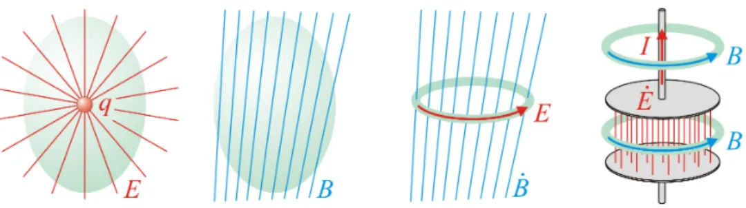
Figure 1:

An illustration of Maxwell’s equations. A chargeqcauses an electric fieldE, while there are no magnetic charges. A time-varying magnetic field ˙B causes an electric field, while a time-varying electric field ˙E gives rise to a magnetic field, and so does a currentI.

machine code. Compiled code, as in FORTRAN or C, executes much faster than interpreted in- structions but this is not critical for the programs written in the context of this course. Libraries like NumPy [6], SciPy [7]and Matplotlib [8] make PYTHON attractive for scientific computing, providing mathematical functions, fast processing of arrays, and MATLAB-like plotting tools.

1.2 Review of electromagnetism

Most of the phenomena and methods studied in this course are accounted for by classical electro- dynamics, the basis of which are the Maxwell equations first published in 1865 [9]. In vacuum, they read

div E ~ = ρ ε

0

or

I

A

E d~a ~ = q ε

0

(1) div B ~ = 0 or

I

A

B d~a ~ = 0 (2)

rot E ~ =

−

∂ ~ B

∂t or

I

S

E d~ ~ s =

− I

A

∂ ~ B

∂t d~a (3)

rot B ~ = 1 c

²

∂ ~ E

∂t + µ

₀

~j or

I

S

B d~ ~ s = 1 c

²

I

A

∂ ~ E

∂t d~a + µ

₀ I

A

~j d~a. (4) In a few words (and see also Fig.1):

•

In the differential form, an electric charge density ρ acts as source or drain of an electric field E. In the integral representation, you may say that the charge ~ q accounts for an electric flux (field times area) through a surrounding area A. If this was the whole story, electric field lines would always begin or end at charges.

•

There is no counterpart to the electric charge for the magnetic field B ~ , and this asymmetry

seems a bit odd. However, the magnetic field can be shown to be a relativistic effect caused

by moving charges, even if they move slower than 1 mm/s through a copper wire. Due to the absence of a magnetic charge, magnetic field lines are always closed loops.

•

The rotation of an electric field, allowing for closed electric field lines, is caused by a time- varying magnetic field. In integral form, a non-zero line intergal

^H

B d~ ~ s along any closed loop (not neccessarily following a field line) is caused by a variation of magnetic flux within the enclosed area A. This is the so-called induction law.

•

The rotation of a magnetic field is caused by a time-varying electric field. Equivalently, the line intergal

^H

E d~ ~ s along any closed loop is caused by a variation of the enclosed electric flux. In addition, the rotation or non-zero line integral can be caused by moving electric charges, expressed either by the current density ~j or by the enclosed current I =

^H

~j d~a.

The second term of this equation is Ampere’s law.

In SI units, which will be used throughout this course, the dielectric constant ε

0

= 8.854

·

10

⁻¹²

C

²

J

⁻¹

m

⁻¹

and the free-space permittivity µ

₀

= 4π

·

10

⁻⁷

Vs/(Am) with ε

₀

µ

₀

= 1/c

²

are inevitable. This makes some formulas look less elegant than in, e.g., the CGS system, but helps to avoid ridiculous units (unless you prefer to measure the electric resistance in s/cm rather than Ohm). The electric charges q, in case you didn’t know, always come in integer multiples of the elementary charge, which is e = 1.602

·

10

⁻¹⁹

C in SI units (or 4.8·10

⁻¹⁰

g

^1/2

cm

^3/2

s

^−1/2

in CGS units).

The force exerted by electric and magnetic fields onto a charge q is the Lorentz force

F ~ = q

·

E ~ + q

·

~ v

×

B, ~ (5) where ~ v is the velocity of the charge. The magnetic field acts only on a moving charge, and pulling perpendicularly to ~ v, it can only change the direction of its velocity. The electric field always acts on a charge, whether it moves or not, and pulls it in the direction of the field (in fact, the force defines the field E ~ = F /q). ~

Electric fields are measured in N/C or equivalently in V/m (since 1 V = 1 J/C = 1 Nm/C). In electrical engineering, tens of MV/m are commonly attainable. In short laser pulses, the electric field can be many GV/m or even TV/m. Note that static electric fields are limited in air to about 3 MV/m, above which the air is ionized and an avalanche discharge occurs.

Magnetic fields are measured in T (Tesla). Recall that 1 T = 1 Vs/m

²

. A permanent magnet (typically SmCo or NdFeB) can reach almost 2 T on its surface, similar to electromagnets made of wires wound around iron cores. Higher fields are obtained by superconducting magnets, e.g.

the 1232 dipole magnets of the Large Hadron Collider (LHC) at CERN have a field of 8.4 T. In dedicated high-field labs, pulsed magnetic fields of the order of 100 T are obtained. And if this is not enough, you find 10

⁸

T in the vicinity of a neutron star.

While the electric field is defined as the force acting on a unit charge, the electrostatic

potential φ is the energy gained or lost by moving a unit charge from one point in the electric

field to another. More formally: if the rotation of a vector field E ~ is zero everywhere, it can be described as gradient of a scaler field

∇ ×

~ E ~ = 0

→

E ~ =

−∇φ,

~ (6) where the minus sign is a matter of convention and any constant may be added to the potential. Inserted into Eq. 1, this leads to Poisson’s equation

∇

~

²

φ =

−

ρ ε

0

(7) or Laplace’s equation in the case of ρ = 0. If the divergence of a vector field such as B ~ is zero everywhere, it can be described as rotation of a vector field

∇

~ B ~ = 0

→

B ~ =

∇ ×

~ A. ~ (8) The gradient of a scalar field may be added to A. With ~

∇ ×

~ B ~ =

∇(

~

∇ ·

~ A) ~

−∇

~

²

= µ

₀

~j and choosing

∇ ·

~ A ~ = 0, a Poisson-like equation is obtained from Ampere’s law

∇

~

²

A ~ =

−µ₀

~j. (9) In the context of radiation, we will encounter

retarded

potentials, meaning that the potential at a particular position is not given by the present charge and current distribution, but by the distribution at earlier time, depending on the distance to that position.

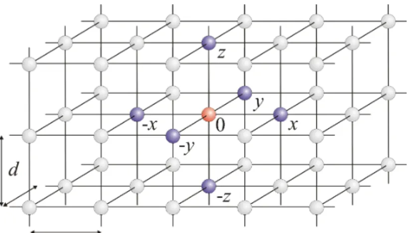
The following consideration may help to give a meaning to the fact that the electrostatic po- tential in free space obeys Laplace’s equation

∇

~

²

φ = 0. In a numerical treatment, the derivative is the difference of φ at two adjacent points divided by the distance between them. The sec- ond derivative is the difference of first derivatives at two points, again divided by the distance.

Considering an equidistant 3-dimensional grid with spacing d (see Fig. 2), a numerical version of Laplace’s equation would read

1 d

φ

+x−

φ

0

d

−

φ

0−

φ

−x

d

+ 1 d

φ

+y−

φ

0

d

−

φ

0−

φ

−y

d

+ 1 d

φ

+z−

φ

0

d

−

φ

0−

φ

−z

d

= 0, (10) where φ

0

is the potential at some grid point and φ

±i

with i = x, y, z are the potential values at adjacent grid points in x, y or z direction. Solving this equation for φ

₀

yields

φ

₀

= 1

6 (φ

_+x

+ φ

−x

+ φ

_+y

+ φ

−y

+ φ

_+z

+ φ

−z

) . (11) At each position, the potential φ is given by the arithmetic mean of the adjacent potential values. The same is true for each component A

i

of the magnetic vector potential in free space.

Could nature have been designed more simple?

Figure 2:

A grid in 3-dimensional space with equal spacingdin each direction. One selected point (0) and two adjacent points in each direction are highlighted.

In this very brief introduction, not all aspects of electromagnetism can be discussed. We come to Ohm’s law, electromagnetic waves, dielectric and magnetic polarization, and other things when need arises.

1.3 Review of special relativity

The velocity of light in vacuum is roughly c = 3

·

10

⁸

m/s (it fact it is

defined

to be exactly 299,792,458 m/s in SI units). It is useful to know typical distances related by the velocity of light to relevant time intervals , e.g.

1 s

←→

300,000 km (a bit less than the distance to the moon)

1 ms

←→

300 km (the distance between the accelerator labs DELTA and DESY) 1 µs

←→

300 m (typical circumference of a circular accelerator)

1 ns

←→

30 cm (typical length of a cable)

1 ps

←→

0.3 mm (length of a laser pulse or particle bunch) 1 fs

←→

300 nm (a bit less than the wavelength of visible light) 1 as

←→

0.3 nm (size of an atom).

The experimental observation that c is the same in any inertial system leads to the Lorentz transformation

x

⁰

= γ (x

−

vt) y

⁰

= y z

⁰

= z t

⁰

= γ(t

−

vx/c

²

), (12)

where the system with primed coordinates moves against the other one in x direction with

constant velocity v. The Lorentz factor is γ = 1/

^p

1

−

β

²

with β = v/c and

Figure 3:

Left – the Bevatron, a proton synchrotron constructed in 1954, with E. McMillan and E.

Lofgren standing on its roof. Right – the B factory at SLAC, an e⁺e⁻ collider fed by the Stanford two- mile linear accelerator, in operation from 1998 to 2008 (both: Copyright Univ. of California, Lawrence Berkeley National Laboratory).

γ

²

= 1

1

−

β

² −→

1

γ

²

= 1

−

β

² −→

γ

²−

β

²

γ

²

= 1 or β

²

γ

²

= γ

²−

1. (13) Special relativity accounts for perplexing phenomena like the Lorentz contraction or time dilatation. Another consequence is that the mass becomes a function of velocity m = m

0

γ with m

₀

being the rest mass, but Newton’s law F ~ = ˙ ~ p = m ~a = m ~ v ˙ still holds. Thus, the relativistic momentum is

~

p = m ~ v = m

₀

γ ~ v = m

₀

γ ~ βc. (14) In particle and accelerator physics, the motion of a particle with charge e in a homogeneous magnetic field is a recurring theme. Setting the centripetal force equal to the Lorentz force (let’s assume ~ v

⊥

B) leads to a relation between momentum, magnetic field and bending radius ~

mv

²

R = p

R v = evB

→

p = eBR or p[GeV/c]

≈

0.3 B[T] R[m] (15) The total energy of an object is its rest energy m

₀

c

²

plus, if not at rest, its kinetic energy T . Useful relations are

E = m c

²

= m

₀

γ c

²

= m

₀

c

²

+ T =

q

m

²₀

c

⁴

+ p

²

c

²

= c

β p. (16)

In particle physics, it is common to use the convention c = 1 which allows to express mass,

momentum and energy in eV (or rather GeV). Here, we resist this temptation and continue with

proper SI units. If it comes to inserting numbers, omitting a factor c

²

in the wrong place causes the result to be off by 17 orders of magnitude.

It is common in special relativity to combine related quantities to a 4-vector, e.g.

P = E

c , p

_x

, p

_y

, p

_z

, (17)

where the product of two vectors follows a peculiar rule. The square of P reads P

²

= E

²

c

² −

p

²_x−

p

²_y

,

−p²_z

= E

²

c

² −

~ p

²

= m

²₀

c

²

. (18) There are variations of this rule in literature, e.g., a minus sign for the energy instead of momentum components or enforcing the minus sign by an additional i. Whatever the details, the square of P turns out to be an invariant, i.e. its value is unchanged under Lorentz transformation.

For a single particle, the ”invariant mass” m

₀

is the rest mass. For multiple particles, it is the highest mass you can create in a particle reaction. Consider, for example, the collision of two particles with rest masses m

1

and m

2

in different reference frames. Of practical interest is e.g.

•

the laboratory system with particle energies E

₁⁰

und E

₂⁰

and momenta p

⁰₁

und p

⁰₂

,

•

the center-of-momentum system in which the sum of momenta p

1

and p

2

is per definition 0 and the sum of energies E

₁

and E

₂

equals m

₀

.

With these definitions, the above-mentioned invariance condition reads

m

²₀

c

²

= 1

c

²

(E

₁

+ E

₂

)

²

= 1

c

²

(E

₁⁰

+ E

₂⁰

)

²−

(p

⁰₁

+ p

⁰₂

)

²

= c

²

(m

₁

γ

₁⁰

+ m

₂

γ

₂⁰

)

²−

c

²

(m

₁

β

⁰₁

γ

₁⁰

+ m

₂

β

₂⁰

γ

₂⁰

)

²

. (19) Consider first fixed-target experiments in which particle 2 is at rest (β

⁰₂

= 0, γ

₂⁰

= 1). For simplicity, both particles may now be protons (m

1

= m

2

= m

p

). Using the relation β

²

γ

²

= γ

²−1

m

²₀

c

²

= m

²_p

c

²

(γ

₁⁰

+ 1)

²−

m

²_p

c

²

(γ

₁⁰²−

1) = 2m

²_p

c

²

(γ

₁⁰

+ 1) . (20) An example is the creation of antiprotons by bombarding a target with protons (p+p

→

p+p+p+¯ p) where m

0

= 4 m

p

and γ

₁⁰

= 7. Thus, a proton beam with a minimum kinetic energy of 6 m

_p

c

²

= 5628 MeV is required to create one antiproton with a rest energy of 938 MeV. In 1954, a 6.2-GeV proton synchrotron, the so-called Bevatron (from BeV, billion electron volts), was built at Berkeley/USA – see Fig. 3. One year later, the antiproton was discovered at this machine.

Experiments with counter-propagating beams use the energy of accelerated particles more

efficiently. For a symmetric collision of protons with β

⁰₁

=

−β₂⁰

, the result is

m

²₀

c

²

= 4 E

₁⁰²

c

²

= 4 E

₂⁰²

c

²

. (21)

Demanding again m

0

= 4m

p

, the required Lorentz factors are γ

₁⁰

= γ

⁰₂

= 2 and the sum of kinetic energies is 1876 MeV. For collision experiments with asymmetric particle energies, the approximation

m

²₀

c

²

= E

₁⁰²

c

²

+ 2 E

₁⁰

E

₂⁰

c

²

+ E

₂⁰²

c

² −

p

⁰₁²

+ 2p

⁰₁

p

⁰₂−

p

⁰₂² ≈

4 E

1

E

2

c

²

(22)

holds for ultrarelativistic particles with p

≈

E/c. In the 1990s, two so-called B-meson factories were built, one at SLAC/USA (Fig. 3), the other at KEK/Japan. In these e

⁺

e

⁻

colliders with asymmetric beam energy, B - ¯ B pairs were abundantly created via the Υ(4S) resonance at m

0

= 10.6 GeV. Thus, the product of the two beam energies was always 28 GeV

²

, e.g. 8 GeV and 3.5 GeV.

1.4 Light and particle optics

The treatment of a light beam in an optical setup and a particle beam in an accelerator or storage ring has much in common, although the wording is quite different by tradition. Here, we try to work out the similarities and come to the differences when discussing the respective instruments.

A ”beam” is a more or less collimated flow of radiation or particles. In either case, beams have become major tools of research ever since the discovery of x-rays and radioactivity. Consider, for example, the discovery of the atomic nucleus with α-particle scattering by E. Rutherford in 1911 [10] or X-ray crystallography pioneered by M. v. Laue in 1912 [11].

Particle beams are usually characterized by their kinetic energy (for high-energy electrons, though, the difference between kinetic and total energy is insignificant) and the beam current, i.e. the charge q passing a particular position per time interval. Note that in a storage ring, the same charge goes around many times per second. Thus, the measured current is given by q

·

f

rev

, charge times revolution frequency (e.g. f

rev

= 2.6 MHz at DELTA, f

rev

= 11 kHz at the LHC).

Electromagnetic radiation is specified by its wavelength λ, the corresponding frequency ν = ω/(2π) = c/λ, or by the photon energy E

γ

= h ν = ¯ h ω. It is useful to know Planck’s constant h as well as ¯ h = h/(2π) in different units:

h = 6.626

·

10

⁻³⁴

J s = 4.136

·

10

⁻¹⁵

eV s, ¯ h = 1.055

·

10

⁻³⁴

J s = 6.582

·

10

⁻¹⁶

eV s

(depending on context, combinations of constants like ¯ hc

≈

197 MeV fm may also be useful

to memorize). The intensity of radiation may be given in terms of power (in W) or photons per

time unit (s

⁻¹

), both of which may be normalized to an area (in m

²

), an angle (rad), a solid

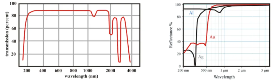
Figure 4:

Left – typical transmission curve of light through glass (here UV grade fused silica, consisting of amorphous quartz SiO₂ and optimized for good UV transmission). Right – reflectivity of aluminium, silver and gold (after Wikipedia, author Bob Mellish). The reduced reflectivity of gold below 500 nm causes its color. As the figure shows, aluminium is a good choice for broadband mirrors in the UV range.

angle (rad

²

) and/or an absolute spectral interval (e.g. in eV or nm) or a relative bandwidth (typically 1 % or 0.1 %).

1.4.1 Guiding and focusing beams

Once created, beams are deflected and focused in order to direct them towards their destination.

The method of doing so as well as the setup is referred to as ”optics”. Note that the transport of beams often requires vacuum, which is nearly always the case for particle beams. Visible light (defined by a wavelength range from 400 to 700 nm) propagates in air, as we know from daily experience. Ultraviolet (UV) light is strongly absorbed below 200 nm and therefore called vacuum UV (VUV) in that regime, infrared (IR) light above 1000 nm suffers from numerous absorption bands caused mainly by H

2

O, O

3

, and CO

2

.

Light is deflected by flat mirrors or prisms, and it is focused by lenses, curved mirrors, or just by a pinhole. For many appliciations, prisms and lenses do not work since their material is not transparent to particular wavelengths. Glas-like materials are typically opaque below 150 nm and above a few µm (see Fig. 4), and become transparent again at very long wavelengths. Hard X-rays are transmitted by any material if it is thin enough. For lenses, the index of refraction n must be different from that of the environment. For visible light, glas with n

≈

1.5-1.9 is usually surrounded by air n

≈

1. In the case of X-rays, the refractive index of a material can be slightly below 1, and air lenses surrounded by a transparent material, e.g. beryllium, are sometimes employed.

Other reasons to avoid the transition through material may be distortions by dispersion (for broadband radiation) or by the intensity dependence of the refractive index (for intense pulses;

more on that later). Mirrors also have their limitations. The reflectivity depends on the material,

the quality of the surface, the wavelength (Fig. 4) and the angle of incidence. In synchrotron

radiation beamlines, X-rays are usually deflected and focused by mirrors at grazing incidence

(small angle between ray and surface).

The focusing property of a curved mirror derives from the law of reflection (also called specular reflection), saying that incident and reflected rays have the same angle with respect to the surface normal. The effect of a lens is due to Snell’s law sin θ

1

/ sin θ

2

= n

2

/n

1

, relating angles of incidence θ

_i

and refractive indices n

_i

of two materials (i = 1, 2) to each other. In both cases, there is a focal length f for perpendicular incidence, defined as the distance from the mirror/lens to the point at which initially parallel rays meet. The quantity 1/f is known as optical power or refraction power. The focal length f

_M

of a spherically curved mirror and the focal length f

_L

of a lens are related to the respective radii of curvature according to

1 f

M

=

−

2 R

1 f

L

= (n

−

1)

1

R

1

−

1 R

2

+ (n

−

1)d nR

1

R

2

. (23)

For a lens, the relation is more complicated since there are two surfaces which may have different radii R

i

, a non-negligible distance d from each other, and there is a refractive index n

6= 1. Note that the radii have a sign depending on the orientation of the curvature. Deviating

from normal incidence, the focal length is different for the plane containing the beam and the optical axis (the meridional plane) and the plane perpendicular to it (the sagittal plane). The focal length can only be kept constant by a variation of the radius of curvature. The shape of the mirror is then a toroid or an elliptical paraboloid.

Particle beams are deflected by the homogeneous electric field between two capacitor plates or by the homogeneous magnetic field in a dipole magnet, and they are focused by electrostatic or magnetic lenses. Electrostatic fields are only effective for low particles velocities, e.g. in electron microscopes, photoelectron spectrometers or low-energy accelerators. As the velocity approaches c, the force of a 1-T magnet corresponds to that of an unrealistic electric field of 300 MV/m (see Eq. 5). The sequence of magnets in an accelerator or storage ring is often referred to as the ”lattice”. A singular application of electrostatic deflection in high-energy accelerators is the pretzel scheme, used e.g. at the e

⁺

e

⁻

collider CESR of the Cornell University in Ithaca/NY/USA.

The unwanted (”parasitic”) collisions of the beams counter-propagating with equal energy and opposite charge in the same magnetic lattice cannot be prevented by magnets since e~ v

×

B ~ always points in the same direction. Other than that, magnets are preferred to guide and focus particle beams. A drawback of magnets with an iron yoke is hysteresis leading to different B values for the same coil current. This may be minimized by ”cycling”, i.e. ramping the magnets repeatedly in a defined way before setting the final value.

An electrostatic lens is typically designed as a cylinder with a gap at which the curved electric

field has a focusing effect. High-energy particle beams are focused by quadrupole magnets with

two north and two south poles. At its center, the quadrupole field is zero and increases linearly

with transverse offset. Quadrupoles focus a beam in one plane while defocusing the beam in the

perperndicular plane. At least two quadrupoles with opposite polarity are required to focus in

both planes.

The deflection of light by a prism depends on the wavelength, the deflection of particles in a magnet on their energy. In both cases, the term ”dispersion” is used, albeit with different definitions.

For electromagnetic radiation, dispersion is defined by dn/dλ, the dependence of the index of refraction on the wavelength, which is related to the spectral dependence of the velocity of light v, since n = c/v. For light in matter, this dependence is due to the resonant behavior of atomic electrons in the presence of an oscillating electric field. Resonances often occur in the ultraviolet (UV) regime, thus blue light is slowed down more than red light (so-called ”normal” dispersion).

If the wavelength is not negligible compared to the size of the surrounding boundaries, e.g. for a radiofrequency (RF) signal in a waveguide or light in an optical fiber, dispersion is also caused by geometric resonant effects (”modes”).

For particles with charge e, their momentum p and bending radius R in a magnetic field B are related according to p = eBR (see Eq. 15), leading to momentum-dependent and thus energy- dependent trajectories. In accelerator physics, the dispersion D is defined via ∆x = D

·

∆p/p, the transverse deviation of an off-momentum particle from the design trajectory, where ∆p is the deviation from the design momentum p. Here, dispersion is not a property of a single magnet, but of the whole lattice. More loosely defined is the ”longitudinal dispersion” of particles, referring to the momentum dependence of the path length.

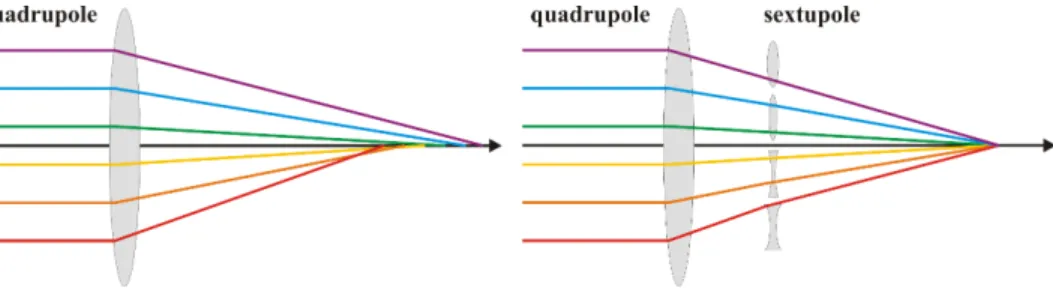
Dispersion also influences the focusing properties in both cases. A lens usally focuses blue light stronger than red light. An ”achromatic” lens would focus light of all colors in the same way, which can be achieved by an ingenious combination of different lenses. In accelerator physics, an achromatic lattice is a combination of dipole and quadrupole magnets that deflects particles of slightly different energy (usually in the sub-percent range) in the same way. In other words, if the disperion (the accelerator version of it) is zero at the beginning of that lattice, it is also zero at its end. The focusing of particles is a different story. Of course, the focal length of a quadrupole magnet depends on the particle momentum or energy. The higher the energy, the ”stiffer” the beam, the longer the focal length. The equivalent to an achromatic lens is to use sextupole magnets in a dispersive region. Just as a quadrupole can be viewed as a transversely position- dependent dipole, a sextupole can be viewed as a position-dependent quadrupole. Dispersion D

6= 0 implies a correlation between momentum and transverse coordinate, and a sextupole

field is arranged such that particles with higher energy experience additional focusing while those with lower energy are defocused (see Fig. 5).

1.4.2 Ray tracing

Much of optics design work involves tracing of either light ”rays” or particles through a setup

of lenses or magnets, respectively. A light ray is an idealized concept within the framework

of geometric optics in which diffraction is ignored. It is nevertheless useful to understand the

transport of light through an optical setup. Although wave-particle duality tells us that particles

are also subject to diffraction, wave phenomena are negligible in accelerators and the ray concept

Figure 5:

Schematic view of a quadrupole magnet in the presence of dispersion, i.e. the (color coded) particle energy depending on the transverse coordinate. Particles of lower energy (red) undergo stronger focusing than those of higher energy (violet). This can be corrected by a sextupole magnet, which acts as a position-dependent quadrupole.

almost perfectly describes the propagation of particles. Deviations, however, may occur due to the Coulomb repulsion between charged particles. These ”space charge” effects are strong for low-energy beams but vanish for highly relativistic particles since in this limit the Coulomb repulsion is balanced by the magnetic attraction between co-moving charges.

The treatment of light rays and particle trajectories is very similar. Therefore, we use the nomenclature of accelerator physics:

s is the position along an axis in beam direction,

x is the horizontal position perpendicular to the direction of s, y is the vertical position perpendicular to the direction of s,

x

⁰≡

dx/ds is the horizontal angle in the limit of small angles (tan α

≈

α), y

⁰ ≡

dy/ds is the vertical angle.

The ”axis in beam direction” may be the optical axis of a setup, e.g. passing through the centers of lenses. At a mirror, the direction of s changes abruptly, and so do the x and y directions, always being perpendicular to s. In the case of an accelerator or storage ring, the axis in beam direction is the design orbit, usually passing through the quadrupole centers. It can be thought of as the trajectory of a reference particle, with respect to which all other particles perform longitudnal and transverse oscillations. A light ray or particle trajectory is given by a vector of transverse positions and angles as function of s:

R(s) = ~











x(s) x

⁰

(s) y(s) y

⁰

(s)











or X(s) = ~ x(s) x

⁰

(s)

!

and Y ~ (s) = y(s) y

⁰

(s)

!

. (24)

For many purposes, the horizontal and vertical plane can be treated independently and it is

sufficient to consider either X ~ or Y ~ alone. These vectors are transformed from one position s

1

to another position s

2

> s

1

by so-called transport or transfer matrices. In ray optics, they are also known as ABCD matrices. In general

x(s

₂

) x

⁰

(s

2

)

!

= A B

C D

!

·

x(s

₁

) x

⁰

(s

1

)

!

. (25)

For a free space (also called drift space in accelerator physics) of length L, the transfer matrix is very simple, representing two equations, one stating that x(s) follows a straight line, the other saying that x

⁰

(s) is constant:

x(s

₂

) x

⁰

(s

₂

)

!

= 1 L

0 1

!

·

x(s

₁

) x

⁰

(s

₁

)

!

. (26)

For a lens of focal length f in thin-lens approximation s

₁ ≈

s

₂

, the matrix keeps x(s) constant while changing the angle:

x(s

₂

) x

⁰

(s

2

)

!

= 1 0

−1/f

1

!

·

x(s

₁

) x

⁰

(s

1

)

!

. (27)

Here, positive/negative f corresponds to a focusing/defocusing lens, making the absolute value of the angle x

⁰

smaller/larger. The same equation holds for the vertical vector Y ~ (s).

Transfer matrices may be combined by matrix multiplication, e.g. a telescope of lenses with focal lengths f

₁

and f

₂

separated by a distance L is described by

x(s

₂

) x

⁰

(s

₂

)

!

= 1 0

−1/f₂

1

!

·

1 L 0 1

!

·

1 0

−1/f₁

1

!

·

x(s

₁

) x

⁰

(s

₁

)

!

(28)

= 1

−

L/f

1

L

−1/f₁−

1/f

₂

+ L/(f

₁

f

₂

) 1

−

L/f

₂

!

·

x(s

1

) x

⁰

(s

₁

)

!

.

Note that f

1

and f

2

can be positive or negative and the combined matrix already describes a number of optical instruments, e.g. an achromatic lens system, a Galilean telescope (a focusing and a defocusing lens), a Keplerian telescope (two focusing lenses), or a simple microscope.

In contrast to ray optics, it is not very common to use the thin-lens approximation in accel-

erator physics. The longitudinal extension of quadrupoles is not negligible, and since particle

tracking is usually done by computer codes rather than by back-of-the-envelope calculation,

there is no need to sacrifice accuracy for simplicity. Thus, the matrix of a focusing quadrupole

magnet (given here without derivation) looks a bit more complicated than that of a lens, but

the thin-lens approximation reveals their similarity:

x(s

2

) x

⁰

(s

₂

)

!

= cos

^p|k|L √¹

|k|

sin

^p|k|L

−^p|k|

sin

^p|k|L

cos

^p|k|L

!

·

x(s

1

) x

⁰

(s

₁

)

!

≈

1 0

−|k|L

1

!

·

x(s

1

) x

⁰

(s

₁

)

!

. (29) Here,

|k|

is a quantity measuring the strength of the quadrupole, and k can be positive or negative to encode whether the magnet focuses in the horizontal or vertical plane. For the thin-lens approximation, cos α

≈

1, sin α

≈

0, and sin α

≈

α for small α has been used.

Another difference to ray optics is that a horizontally focusing quadrupole is inevitably a vertically defocusing magnet and the transformations for the position vectors X ~ and Y ~ are different. With the equation for X ~ as above, the corresponding equation for Y ~ reads

y(s

₂

) y

⁰

(s

₂

)

!

= cosh

^p|k|L √¹

|k|

sinh

^p|k|L p|k|

sinh

^p|k|L

cosh

^p|k|L

!

·

y(s

₁

) y

⁰

(s

₁

)

!

≈

1 0

|k|L

1

!

·

y(s

₁

) y

⁰

(s

₁

)

!

.

(30)

1.4.3 The beam waist

A beam can be thought of as the entirety of many individual rays, and a beam waist (at which the beam diameter has a local minimum) is a good example to inspect the similarites and differences between light and particle optics.

In both cases, beams are often considered as normal (or Gaussian) distributions of intensity or particle density. In geometrical optics, any distribution of parallel rays becomes pointlike in the focus of a lens. In practice, a pointlike beam spot is prevented by the wave properties of light, i.e. by diffraction. In the literature of optics and lasers, the waist of a Gaussian beam is usually described as

w(z) = w(0)

s

1 + z

²

z

_R²

with z

R

= πw

²

(0)

λ , (31)

where the longitudinal position is z (instead of s), w(z) is the beam radius, λ is the radiation wavelength, and z

R

is the so-called Rayleigh length. At a distance of one Rayleigh length from the waist (z = z

R

), the radius has increased by a factor of

√

2, and in the far field (where the first term is negligible), the beam divergence is given by w(0)/z

_R

. In this equation, the beam radius is expressed as the transverse distance at which the intensity is 1/e

² ≈

0.135 of the maximum.

For a Gaussian distribution, w is thus equal to twice the standard deviation:

1

e

²

= e

^−12w

2

σ2 →

ln 1

e

²

= ln 1

−

2 ln e =

−2 =−

1 2

w

²

σ

² →

w = 2σ. (32)

Returning to the notation of accelerator physics with s instead of z and σ instead of w, Eq. 31

reads

2σ(s) =

s

4σ

²

(0) + 4σ

²

(0) λ

²

16π

²

σ

⁴

(0) s

²

or σ(s) =

s

σ

²

(0) + λ

²

16π

²

σ

²

(0) s

²

. (33) In accelerator physics, the root-mean-square (rms) size of particle beams, e.g. in a storage ring, is given by

σ(s) =

q

εβ(s), (34)

where ε is the so-called emittance, which is constant over the entire machine, and β(s) is the amplitude function (or just called ”beta function”) describing the variation of beam size with s.

Since the beam is usually not round, all quantities should actually carry an index x or y, which has been omitted here for brevity. For a beam waist, the beta function has a local minimum.

The transformation rules for the beta function say that it grows from a beam waist at s = 0 according to β(s) = β(0) + s

²

/β(0). The beam size is thus

σ(s) =

s

εβ(0) + ε 1 β(0) s

²

=

s

σ

²

(0) + ε

²

σ

²

(0) s

²

. (35) Comparison with Eq. 33 suggests that the emittance of a particle beam is formally related to the diffraction limit of a light beam by ε = λ/(4π), and sometimes an emittance is assigned also to radiation according to this formula. However, it should be clear that the emittance of a particle beam is not a diffraction effect. While the wavelength of radiation constitutes a fundamental limit on the size of a beam waist, the emittance of a particle beam is given by practical issues. For linear accelerators, the emittance is limited by the quality of the particle source and space charge effects at low energies. In electron storage rings, the emittance assumes an equilibrium value between two effects related to synchrotron radiation (more later), and as a general rule, the bigger the machine, the smaller the emittance can be made. The size of a particle beam is usually far from fundamental limits.

1.5 Processing electrical signals

Most instruments produce electrical signals that are processed in some way, digitized and fur- ther analyzed offline. Even astronomers don’t just gaze at stars anymore, but control their telescopes remotely – maybe even from a different continent – and record data with pixel detec- tors and spectrometers. This section provides some introductory remarks that apply to many instruments. An excellent book on the topic is [12].

1.5.1 Pulsed signals

Electrical signals may be continuous like the current from a microphone. In contrast to that,

signals from detectors and many other instruments are often pulsed. These pulses may be

unipolar (only one polarity) or bipolar (both polarities with a zero-crossing), they may be analog (encoding information in their height, shape, or duration) or digital (only signifying bit 1 or 0 by their presence or absence).

Measured from a baseline to which the pulse eventually decays (zero or some constant voltage or current), a pulse has a height, a width, a rise time at its leading edge, and a fall time at its trailing edge.

The signal width is usually taken as the full width at half-maximum (FWHM) of the pulse height or – more common for Gaussian pulses – as the standard deviation from its centroid, also called root-mean-square (rms) of the deviation. For Gaussian pulses, the FWHM width ∆t of a pulse is related to its rms value σ

t

by ∆t = 2

√

2 ln 2 σ

t≈

2.35 σ

t

. Rise and fall times are usually quoted as the time interval between 10% and 90% of the amplitude along their leading or trailing edge.

In practice, not all aspects of an analog pulse are of interest. For example, its height may encode the energy of a particle, the intensity of radiation, or some other continuous quantity, while the pulse width is of no concern as long as it does not change. Sometimes merely the presence of a pulse is relevant, e.g. the signal from a Geiger-M¨ uller counter which does not contain other information than the occurrence of a particle.

Digital pulses encode one of several states. In most cases, there are only two states corre- sponding to a binary digit (0 or 1) or logic information (yes/no, on/off, ok/faulty, and the like).

Depending on whether a voltage or current exceeds a defined threshold, the signal is assumed to be present or not. Typical standards for digital signals are (from slow to fast):

•

TTL (Transistor-Transistor Logic) ”0” between 0 and +0.8 V, ”1” between +2 and +5 V,

•

NIM (Nuclear Instrumentation Module) ”0” within

±1 mA, ”1” between -12 and -32 mA,

•

ECL (Emitter-Coupled Logic) ”0” between -5.2 and -1.4 V, ”1” between -1.2 and 0 V.

For a standard resistance of 50 Ω, the NIM logical ”1” is around -1 V. You may find slightly different definitions in the literature, also depending on whether the measurement is performed at the input or output of a device. If signals are not too distorted by noise or impedance mismatch (see below), they are usually well-centered within the allowed range. Typical rise times are 10 ns for TTL, a few ns for NIM, and even below 1 ns for ECL.

1.5.2 Cables and connectors

Electrical signals are transported in various ways, ranging from sub-100-nm lines on a microchip

to inch-sized coaxial cables. However, for not too fancy applications, there are only a few

standard cables and connectors to be known. The cable you are most likeley to step on in a

physics lab is the RG-58, a coaxial cable of 50 Ω impedance, usually about 6 mm thick with a

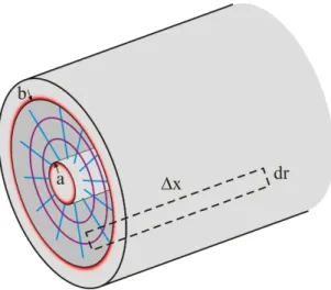
Figure 6:

Cables from a physics lab, each with a male connector and a female-female adapter next to it. From left to right: BNC (with two different sheaths), LEMO 00, Type N, and SMA (with semi-rigid and flexible cable).

black coating and two male BNC connectors at either end

¹

. Another popular 50-Ω coaxial cable is RG-174 with LEMO 00 connectors. These two types of connectors are shown in the left part of Fig. 6, where BNC has a turnable bayonet (”BNC” means Bayonet Neill-Concelman after its inventors) while the LEMO 00 (”LEMO” is a company name) has a push-pull mechanism. The right part of the figure shows two typical connectors for RF signals, the Type N (same as the

”N” in BNC) and the smaller SMA (Sub Miniature version A) connector. Both are threaded, and the Type N is tightened by hand while a small torque wrench is sold to properly tighten the SMA connector.

Cables consist of one or more conducting wires, usually made of copper and surrounded by some insulating material. The standard case is two conductors (for plus and minus, signal and ground etc.), but there may be more, e.g. ribbon cables have up to 96 wires. In order to minimize electromagnetic pickup, cables may be shielded, they may be twisted pairwise, or they may be coaxial.

A coaxial cable consists of two concentric conductors with some material inbetween and the outer conductor is surrounded by an insulating jacket. Flexible cables have a braided outer conductor while the inner conductor is a thin solid wire or also braided. For RF applications, there are ”semi-rigid” cables with a thin copper tube of up to 5 mm diameter as outer conductor, which can be bent to a certain degree without buckling. If the outer copper tube is larger, the cable is completely rigid. The material between the two conductors, usually a dielectric like polyethylene, keeps the inner conductor mechanically centered but also determines the characteristic impedance of the cable.

Some properties of two-wire cables can be found by considering the schematic representation of Fig. 7. Here, the cable has a resistivity R

⁰

= R/∆x per length ∆x, an inductance L

⁰

= L/∆x, a conductivity G

⁰

= G/∆x and capacitance C

⁰

= C/∆x between the conductors. With Kirchhoff’s circuit laws, Ohm’s law, U = L I ˙ , Q = C U and I = ˙ Q, the voltage and current difference is

1It is internationally accepted lab jargon that a connector with a pin sticking out is called ”male” and a connector with a hole matching that pin is called ”female”.

Figure 7:

Equivalent circuit for a piece of two-wired or coaxial cable with resistanceR⁰ and inductance L⁰ along the cable, and conductivityG⁰ and capacitanceC⁰ between the conductors. All quantities are normalized to a length of ∆x, e.g. R⁰ =R/∆x.

U (x + ∆x, t)

−

U (x, t) = ∆U =

−R⁰

∆x I

−

L

⁰

∆x I ˙ (36) I(x + ∆x, t)

−

I (x, t) = ∆I =

−G⁰

∆x U

−

C

⁰

∆x U ˙ (37) along the length ∆x, and for the limit ∆x

→

0

∂U

∂x =

−R⁰

I

−

L

⁰

I ˙ and ∂I

∂x =

−G⁰

U

−

C

⁰

U ˙ (38) Differentiating the first equation with respect to x and inserting the second equation for

∂I/∂x yields

∂

²

U

∂x

²

= L

⁰

C

⁰

U ¨ + L

⁰

G

⁰

+ R

⁰

C

⁰

U ˙ + R

⁰

G

⁰

U

⁰

(39) and a similar equation for I , both of which are known as the telegraph equations. Inserting a general exponential solution U (x, t) = U

0

exp(iωt

−

γx) and dividing by U results in

γ

²

=

−ω²

L

⁰

C

⁰

+ iω L

⁰

G

⁰

+ R

⁰

C

⁰

+ R

⁰

G

⁰

= R

⁰

+ iω L

⁰

G

⁰

+ iω C

⁰

. (40) With γ being a complex number and γ =

±^p

γ

²

, the solution can be written as

U (x, t) = U

₀

exp(iωt

±

γx) = U

₀

exp(±αx) exp(iωt

±

iβx), (41)

where the real part α causes attenuation, and the imaginary part β can be identified as

the wave number k = 2π/λ of a wave travelling in positive or negative direction. The explicit

expression of α as function of frequency ω is a bit complicated and is only significant at low

frequencies in the kHz range. In the more interesting MHz and GHz regime, the attenuation is

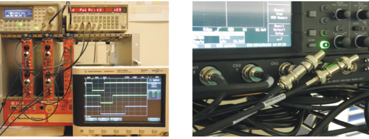
Figure 8:

Due to the skin effect, the current flow (red) is limited to a thin layer near the outer radiusa of the inner conductor and the inner radiusb of the outer conductor. The electric field is shown in blue, the magnetic field in magenta. The area ∆x·dris used to calculate the inductance.

given by another effect: The current flows only through a thin layer beneath the surface of a conductor. Its thickness, the so-called skin depth is given by

δ =

s

2

ωµ

₀

µ

_r

σ , (42)

where µ

0

is the free-space permeability, µ

r ≈

1 is the relative permeability of the conductor, and σ is the specific conductivity. For the current flowing through an area 2πaδ under the outer surface of the inner conductor and 2πbδ under the inner surface of the outer conductor with a and b being the respective radii, the resistivity per meter is

R

⁰

= R

∆x = ∆x

σ 2π δ ∆x 1

a + 1 b

=

r

ω µ

0

8π

²

σ 1

a + 1 b

, (43)

increasing with the square root of the frequency. From this and other considerations, an optimum ratio b/a

≈

3.6 can be derived (see Eq. 52 below).

We will now compute the inductance L

⁰

and capacitance C

⁰

per unit length for a coaxial cable with the radii a and b defined as before (see Fig. 8):

L

⁰

= L

∆x = φ

I ∆x and C

⁰

= C

∆x = Q

U ∆x = λ

U , (44)

where φ is the magnetic flux (magnetic field B times area), and Q is the charge along ∆x.

Assuming a dielectric material with ε

r 6= 1 and

µ

r ≈

1 between a and b, the electric and magnetic

field as function of distance r from an ”infinite” wire with current I and longitudinal charge density λ is

B = µ

₀

2π I

r and E = 1

2πε

0

ε

r

λ

r , (45)

from which the magnetic flux and voltage follows

φ = ∆x

Z b

a

B dr = ∆xµ

₀

I 2π

Z b a

1

r dr and U =

Z b

a

E dr = λ 2πε

₀

ε

_r

Z b a

1

r dr. (46) With

^R_a^b

(1/r)dr = ln(b/a) in both equations, the final result is

L

⁰

= µ

0

2π ln b

a and C

⁰

= 2π ε

0

ε

r

1

ln(b/a) , (47)

which will be used below to calculate the impedance of the cable. To this end, the case of a lossless cable will be considered by omitting all terms containing R

⁰

or G

⁰

in Eqs. 39 and 40:

∂

²

U

∂x

²

= L

⁰

C

⁰

U ¨ γ

²

=

−ω²

L

⁰

C

⁰

(48) from which γ = iω

√

L

⁰

C

⁰

and wave number k = ω

√

L

⁰

C

⁰

follows. Here, the phase and group velocity, ω/k and dω/dk, are both equal to v = 1/

√

L

⁰

C

⁰

. As a rule of thumb, the signal velocity in a typical coaxial cable corresponds to about 1 m in 5 ns, significantly slower than the velocity of light (which would be 1 m in 3.33 ns). Using a lossless version of Eq. 38

∂U

∂x =

−L⁰

I ˙ or γU = L

⁰

iω I (49) with ∂U/∂x =

−γU

and ˙ I = iω L

⁰

according to Eq. 41, the impedance of a cable is given by the ratio of voltage and current

Z = U

I = iω L

⁰

γ = iω L

⁰

iω

√

L

⁰

C

⁰

=

s

L

⁰

C

⁰

. (50)

Thus, the impedance is a real quantity (at least in the lossless approximation) measured in Ω (Ohm). It is independent of the cable length (in contrast to the Ohmic resistance) and independent of frequency (in contrast to the inductance and capacitance). Applying this rather astonishing result to the case of a coaxial cable by inserting Eqs. 47 yields

Z = 1 2π

r

µ

₀

ε

0

ε

r

ln b

a

≈

60 Ω 1

√

ε

r

ln b

a . (51)

A criterion for optimizing the ratio b/a is to minimize the resistance normalized to the impedance for a given outer radius b. With Eqs. 43 and 51

R

Z

∝

1/a + 1/b ln(b/a) = 1

b

·

b/a + 1

ln(b/a) , (52)

with a minimum at b/a

≈

3.6. This and polyethylene as dielectric material (ε

_r ≈

2.4) makes the value of 50 Ω self-evident. Since the impedance depends only logarithmically on b/a, it is clear that the impedance of a coaxial cable cannot be much different from that value (75 Ω and 93 Ω are also found but not, say, 1000 Ω).

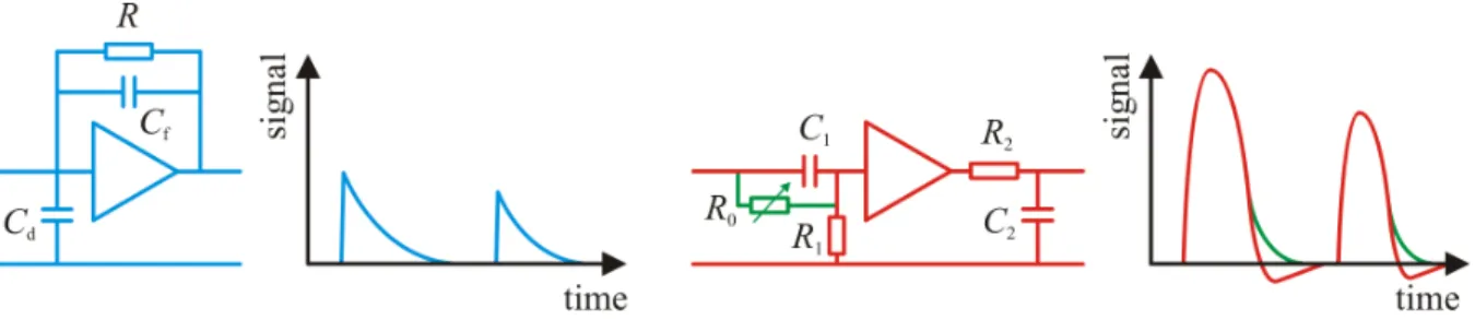
An ohmmeter attached to the two conductors of an open coaxial cable shows infinite re- sistance, not 50 Ω or whatever is written on that cable. The impedance cannot be measured directly, it just happens to be the ratio of voltage to current. You may think that the impedance of free space, which is 377 Ω, is even more mysterious. Why bother at all? Of particular concern are reflections whenever the impedance changes. For example, if a 50-Ω cable is attached to the 1-MΩ input of an oscilloscope, nearly the whole pulse is reflected. Multiple and/or distorted pulses are indications of an impedance mismatch somewhere in your setup. Oscilloscopes may have a 50-Ω option or, if not, a T connector with a terminating resistor can be attached to its input (see right part of Fig. 9). For an oscilloscope input impedance of 1 MΩ, a flat-top pulse will appear with doubled amplitude since the incoming part and the reflected part of the pulse add up. This amplitude-doubling effect is sometimes wanted, e.g. to increase a pulse at the input of an analog-to-digital converter (ADC). In such a case, the ADC has a high input impedance, but the other end of the cable is terminated by 50 Ω to avoid multiple bounces.

1.5.3 Electronics for data acquisition

Electrical signals from any instrument are usually amplified, filtered and/or treated in some other way, and then digitized. The digitized data may again undergo some processing – a mathematical operation (e.g. two signals added, or a baseline value subtracted), being histogrammed, or rejected if they don’t pass some condition – and then stored on a computer disk or other media.

Generally, ”raw data” should not be processed too excessively. For example, it might look like a good idea to store only the sum signal from two counters passed successively by the same particle, but later it may turn out that the individual signals would have been useful (e.g. for particle identification).

Data may be stored in different ways, depending on the type of experiment. In some cases, continuous quantities are sampled at a certain rate and the values

Vi

are stored as function of time

Tk

:

T1 V1(T1) V2(T1) ...Vn(V1) T2 V1(T2) V2(T3) ...Vn(V2) T3 V1(T3) V2(T4) ...Vn(V3)