Instruments of Modern Physics

(1)

– A Primer to Lasers, Accelerators, Detectors and all that

Shaukat Khan, TU Dortmund, Summer of 2014

November 12, 2014

(2)

3 Sources of particle radiation 3

3.1 Particle beam production . . . . 3

3.2 The zoo of particle accelerators . . . . 4

3.3 Longitudinal beam dynamics . . . . 7

3.4 Transverse beam dynamics – particle optics . . . . 10

3.4.1 The equations of motion . . . . 10

3.4.2 Transfer matrices . . . . 12

3.4.3 Optical functions . . . . 13

3.4.4 Momentum-dependent effects . . . . 16

3.4.5 From single particles to particle beams . . . . 17

3.5 Outlook . . . . 17

3.5.1 Beam diagnostics . . . . 17

3.5.2 Beam spectrum and collective effects . . . . 18

(3)

3 Sources of particle radiation

Particle radiation is used for scattering and spectroscopic experiments in nuclear and parti- cle physics, to create new particles and exotic states of matter (e.g. the so-called quark-gluon plasma), and for a number of other purposes e.g. radiotherapy of cancer. Furthermore, particle beams are generated to produce ”secondary” beams, which may be other particles (neutrons, neutrinos, and short-lived particles or nuclei) or photons (synchrotron or FEL radiation). Em- ploying natural sources of particle radiation (particles from radionuclides and cosmic rays) led to a number of important discoveries. However, particles emitted by radionuclides are limited in energy to typical nuclear level differences around 10 MeV. In cosmic radiation, energies up to 10

²⁰

eV were observed, but the flux of these particles is less than one per km

²

and year. The insufficiency of these sources in energy, flux, and other properties triggered the development of particle accelerators.

3.1 Particle beam production

Particle beams are first produced by a particle source (sometimes menacingly called ”gun”), accelerated to the desired kinetic energy, and then either used directly or injected into a storage ring, where the particles can circulate for hours.

Although the following discussion concentrates on accelerators and storage rings, a few re- marks on particle sources shall be made:

• Electron guns are based on thermal emission of electrons from a surface (thermionic guns) or on the photo effect (photocathode guns) due to impinging laser pulses. In either case, the emitted electrons are immediately accelerated by an electric field, which may be static or part of a radiofrequency (RF) wave. Thermionic guns are sufficient for many purposes, e.g. for electrons to be accelerated and injected into storage rings or for linear accelerators in radiotherapy. Short bunches for FELs are mostly produced by RF photocathode guns using short laser pulses, and are further compressed when the electrons have reached higher energies since the Coulomb repulsion decreases with increasing energy.

• There is a variety of proton and ion sources, depending on the way atoms from a gas or vapor are ionized. The most common method is by the collision with electrons, which are accelerated by a static electric field (Penning source), an RF wave from a coil with few windings (RF ion source), or a microwave fed into a resonator overlayed by a static magnetic field in which the electrons perform a circular motion (electron cyclotron reso- nance source). A particular type of discharge tube, known as duoplasmatron, is also in use. Sources of positive ions can also be employed to create negative ions, since colliding electrons not only remove atomic electrons but there is also a chance of electron capture.

Some particle beams have a particular way of production, e.g.

(4)

• Neutrons are created by radioactivity, e.g. mixing an α-emitting nuclide with a material of high (α,n) cross section like beryllium. Another source is nuclear reactions from a proton beam hitting a target, particularly a process called ”spallation”, in which a highly excited heavy nucleus decays by boiling off tens of neutrons. Furthermore, there are nuclear reactors used as parasitic or dedicated neutron sources.

• The creation of antiprotons by bombarding a target with a proton beam (p+p → p+p+p+¯ p) was discussed in Sect. 1.3.

• Pions are also produced by high-energy protons hitting a target.

• A pion beam can be used to create muons and neutrinos via π

⁺

→ µ

⁺

+ν

µ

and µ

⁺

→ e

⁺

+ν

e

(and the analogous reactions for π

⁻

). Nuclear reactors are also used as neutrino sources.

• Positrons are created via pair production, usually in electromagnetic showers from high- energy electrons hitting a target. Instead of electrons, undulator radiation in the MeV range is also under discussion for future e

⁺

e

⁻

colliders.

3.2 The zoo of particle accelerators

This section is meant to convey some basics ideas of particle accelerator physics in a nutshell.

For more details, the reader is referred to the literature, e.g. [1, 2, 3, 4].

As can be seen from the Lorentz force acting on a particle with charge q

F ~ = q · E ~ + q

~ v × B ~

, (1) only an electric field E ~ can change the kinetic energy of the particle, while the magnetic field B ~ causes a centripetal force perpendicular to the particle velocity ~ v. On the other hand, focusing or deflecting a beam of relativistic particles is usually done by magnets, since for v ≈ c the second term with an easily achievable magnetic field of 1 T is as large as the first term with an unrealistically high electric field of 300 MV/m. There are various ways to generate an accelerating electric field:

• An electrostatic field is produced by separating and displacing charges, as e.g. in the Cockroft-Walton generator (Fig. 1, left) by an electric circuit producing a high voltage or in the Van-de-Graaf generator (Fig. 1, center) by mechanical transport of charges.

• According to the law of induction, an electric field is created by a time-varying magnetic

field. So-called betatrons (Fig. 1, right) and induction linear accelerators (”linacs”) are

based on this principle.

(5)

Figure 1:

Sketch of two electrostatic accelerators, the Cockroft-Walton generator (left) using a so-called Greinacher circuit to produce a high voltage, and the Van-de-Graaf generator (center) in which charge is transported mechanically by a belt or chain. The right figure shows the betatron, in which a time-varying magnetic field produces an electric field by induction and keeps the particles (electrons) on a circular path.

• RF fields with typical wavelengths between 0.1 and 1 m (the UHF band) confined to a hollow metallic structure (called cavity or resonator) are the basis of most accelerators.

This is true for circular machines like cyclotrons, microtrons, or synchrotrons, as well as for linear accelerators. Advances in radar technology during World War II, particularly the development of the klystron as an efficient RF amplifier, have made UHF waves useful for particle acceleration with typical electric fields of several 10 MV/m.

• The electric field in a femtosecond laser pulse can reach 100 GV/m and more, but being perpendicular to the direction of propagation, it cannot be used directly to accelerate particles. In 2006, the quest for higher gradients was highlighted by obtaining 1 GeV electrons over an acceleration length of only 3.3 cm with a laser-induced plasma wave [5].

Further progress from LPWA (laser-plasma wakefield acceleration) and other ”advanced”

¹

acceleration schemes can be expected.

While a static electric field accelerates a charged particle only once and the total voltage is limited to the order of 10 MV, standing or propagating RF waves can increase the particle energy repeatedly. In circular accelerators, particles pass through the same RF resonators again and again, while in a linac the beam passes a succession of similar RF structures one after the other, and the achievable beam energy is in both cases mainly given by economic limitations.

Figure 2 shows the generic design of accelerators using RF structures. In circular machines, the magnetic part of the Lorentz force, usually with ~ v ⊥ B, provides centripetal acceleration ~

1 A number of new acceleration schemes with remarkable properties have been devised. In this context,

”advanced” is synonymous to not yet producing useful particle beams (which may change).

(6)

Figure 2:

Schematic view of accelerators based on radiofrequency (RF) waves, (a) the cyclotron, (b) the microtron, (c) the synchrotron, and (d) linear accelerators (linacs). The shaded regions contain a magnetic field, the label ”rf” indicates the locations of accelerating RF structures.

m v

²

R = q v B. (2)

Solving this equation for v/R and considering the relativistic mass m = γm

0

with Lorentz factor γ, the revolution time in a circular machine is

T = 2πR

v = 2πγ m

₀

q B , (3)

which has to be an integer multiple n of the period of the accelerating RF wave, i.e. T = n · T

RF

, which has consequences for the design and functionality of the respective machine.

The cyclotron (first machine 1932 in Berkeley/USA) accelerates non-relativistic particle (medium-energy protons and ions), since the condition T = n · T

_RF

fails for given n when the Lorentz factor in Eq. 3 deviates significantly from 1. As sketched in Fig. 2, the beam path is a spiral with increasing radius R whenever the beam passes the gap containing the RF wave.

Small deviations from γ = 1 can be compensated by a variation of T

_RF

(synchro-cyclotron) or by a radially increasing B field (isochronous cyclotron).

The microtron (first machine 1947 in Ottawa/Canada) is an accelerator with increasing R for relativistic electrons, in which n is not constant. After each pass through a short RF accelerator, the Lorentz factor increases such that n increases in integer steps.

The synchrotron accelerates electrons (first machine 1947 in Berkeley/USA) and hadrons (first machine 1952 in Birmingham/UK) to high energies. All large circular accelerators – like the LHC at CERN and many others – are synchrotrons, since the radius R is kept constant and thus the magnetic field B is only required along the perimeter of its footprint and not over the full area. To keep T nearly constant, the magnetic field and the Lorentz factor are increased synchronously. The drawback of this principle is that, ramping cyclically up and down, it does not allow for continuous operation like the isochronous cyclotron or the microtron.

A storage ring looks like a synchrotron – and some machines like the LHC have both

functions – but the energy of the beam (or counter-propagating beams in the case of a collider)

(7)

is kept constant. Electron/positron storage rings (first machine 1960 in Frascati/Italy) require RF resonators to compensate the energy dissipated by synchrotron radiation, while hadronic rings (first machine 1971 at Geneva/Switzerland) with negligible synchrotron radiation losses only need an RF system when a bunched beam is desired.

The linear accelerator (or linac) is the other type of machine with an economic footprint, while the RF system is much more elaborate than for synchrotrons. The linac principle allows for a continuous beam. In practice, however, most linacs are pulsed with duty cycles (on/off) around 1/100 to keep the RF power and cooling requirements within reasonable limits. The history of particle accelerators started 1928 in Aachen/Germany with the first ion linac, built by R. Wider¨ oe (who had invented the betatron and wanted to build one as his PhD work, but failed [6]). Linacs are essentially circular tubes with a standing or traveling RF wave. For slow particles, they have so-called drift tubes that shield the particles from the RF wave whenever its electric field has the ”wrong” phase. Electron linacs have periodic irises that slow down the phase velocity to values around c to keep relativistic electrons at constant phase

²

.

Cylindrical RF cavities are abundantly used e.g. in synchrotrons and storage rings, and their principle is sketched in Fig. 3 following an argument given in [7]. In contrast to a capacitor with a DC voltage, an electric field oscillating with a frequency of several 100 MHz gives rise to an oscillating magnetic field. The time-varying magnetic field, in turn, modifies the electric field. As a result, the radial distribution of the electric field follows the Bessel function J

0

(kr) with wavenumber k = 2πf /c and radius r. For a frequency of f = 500 MHz (k = 10.5 m

⁻¹

), as an example, the field is zero at r = 0.234 m, since J

₀

(2.45) = 0. A metallic wall at this radius completes the cavity with a so-called transverse magnetic mode TM

010

ringing inside (the subscripts indicate the number of longitudinal, radial and azimuthal nodes of the field).

Many RF cavities are not exactly cylindrical. A smoother bell-like shape (as in Fig. 3 d) reduces the content of higher-order modes (HOMs), i.e. unwanted modes at higher resonance frequencies. It also reduces locally high electric fields, which may give rise to discharges, and high magnetic fields which – in the case of superconducting cavities – lower the critical temperature.

The latter effect limits the accelerating electric field (or voltage gradient) of superconducting cavities to about 50 MV/m in optimized prototypes (30 MV/m in industrial production). The gradient in normal-conducting linacs, limited by cooling and discharge issues, can only be slightly higher.

3.3 Longitudinal beam dynamics

The concept of phase space is widely used in accelerator physics. Particles are described by position and momentum-like variables relative to a reference particle, which may be thought of as a particle flying with the design energy of a machine exactly at the right time along the beam axis. For pulsed beams, it would sit at the center of a particle bunch with nearly Gaussian

2The phase velocity of an electromagnetic wave in a simple cylindrical tube exceedsc, which does not contradict the theory of relativity since the phase of a continuous wave does not carry any information.

(8)

Figure 3:

A parallel-plate capacitor with a DC voltage (a) has – neglecting the fringes – a homogeneous electric field, whereas an AC voltage (b) with wavenumberkcauses the fieldE to follow Bessel’s function J0(kr). A metallic wall at the radius of the first node ofJ0(kr) completes a simple cylindrical (”pillbox”) RF cavity (c). A bell-shaped cavity (d) is more elaborate to manufacture, but has several advantages.

distributions in all coordinates. All other particles tend to perform oscillations about the position of the reference particle. To a certain degree, longitudinal phase space (with the position and momentum component in beam direction), horizontal phase space (usually considering a ”flat”

machine without vertical bending angles) and vertical phase space are decoupled and can be discussed separately.

In longitudinal direction, the position in the laboratory system is usually denoted by s, and it is useful (although not always practiced in the literature) to label the position relative to the reference particle differently, e.g. by z. Instead of z, a temporal variable z/c or – most commonly – the phase Ψ = 2πz/λ

_RF

with respect to an accelerating RF field of wavelength λ

_RF

is used as position coordinate. The momentum-like coordinate is usually ∆p/p, the relative deviation from the design momentum. For highly relativistic particles, the momentum deviation is synonymous to the energy deviation ∆E/E or ∆γ/γ.

For the voltage amplitude V

RF

of a sinusoidal RF field with angular frequency ω

RF

= 2πc/λ

RF

, the energy gain for a particle of charge q is

W = qV

RF

sin Ψ

s

, (4)

where Ψ

s

is the ”design” phase (called synchronous phase in storage rings), which is usually not chosen to yield the maximum energy qV

_RF

for several reasons:

• Longitudinal focusing is provided when the arrival time at an RF structure depends on the momentum deviation such that a particle with too high momentum experiences a reduced accelerating voltage – see below. This requires a voltage slope, i.e. Ψ

_s

6= π/2.

• The concept of bunch compression in linac-based FELs (see Sect. 2.7.4) requires a voltage

slope in order to introduce an energy ”chirp” along the bunch (energy at the tail higher

than at the head of the bunch). The energy-dependent path length in dipole magnets

(9)

can then be used such that the tail of the bunch catches up with the head and the bunch length is reduced.

Deviations from Ψ

_s

cause an oscillation, which is called synchrotron oscillation. If two parti- cles have different momentum, they can change their longitudinal position with respect to each other for different reasons:

• The particle with higher energy is faster, which may not be significant for highly relativistic particles with velocities close to c.

• In a ”chicane”, a detour by magnets leading back to the original beam axis, the particle with higher energy is deflected less and moves forward.

• In a ring-shaped machine, the particle with higher energy is deflected less by dipole magnets and usually (not always) falls behind, because its path is longer. In high-energy storage rings, this effect dominates and is described by the so-called momentum compaction factor α ≡ (∆L/L

₀

)/(∆p/p), the relative deviation from the nominal orbit circumference L

₀

for an off-momentum particle.

The synchrotron motion in a storage ring is rather slow, one oscillation period takes 100 revolutions or more. Similar to electron motion in low-gain FELs under the influence of radiation as shown in Fig. 19 of the previous chapter, synchrotron oscillation under the influence of the RF field is governed by two coupled differential equations. One describes the change of the momentum offset ∆p as function of phase offset ∆Ψ from the synchronous phase, the other describes the change of the phase offset as function of momentum deviation, and the two can be combined to a pendulum equation.

For a particle arriving at the snychronous phase, the energy gained in an RF resonator matches the synchrotron radiation losses W

0

during one turn:

qV

_RF

sin Ψ

_s

− W

₀

= 0. (5)

In the case of hadrons, W

₀

is zero and Ψ

_s

= 0 or π. If the particle velocity is close to c, as assumed in the following, only Ψ

s

= π at the falling voltage slope provides longitudinal focusing:

particles with ∆p > 0 fall behind during one turn and experience a lower accelerating voltage.

For a proton with charge q = e, for example, arriving at a phase Ψ = Ψ

_s

+∆Ψ, the momentum changes by

∆p = eV

RF

c (sin(Ψ

s

+ ∆Ψ) − sin Ψ

s

) = eV

RF

c sin(π + ∆Ψ) = − eV

RF

c sin ∆Ψ (6)

Since the momentum change per turn is small, it can be divided by the revolution time T

₀

to obtain the time derivative

(10)

d

dt ∆p = − eV

RF

cT

0

sin ∆Ψ. (7)

The other differential equation is obtained by considering the temporal change ∆T = T

0

α (∆p/p) over one turn divided by the RF period T

_RF

= 2π/ω

_RF

∆Ψ = 2π ∆T

T

_RF

= 2π T

₀

α

T

_RF

p ∆p = T

₀

ω

_RF

α

p ∆p (8)

and, dividing by T

₀

, the time derivative is d

dt ∆Ψ = ω

_RF

α

p ∆p. (9)

Particles in storage rings usually form bunches with normal distributions along both longi- tudinal phase space axes, while these distributions can be more complex in linacs.

For the case of electrons as illustrated by Fig. 4, the symmetry with respect to Ψ

_s

is broken since the synchrotron radiation loss per turn W

₀

6= 0 has to be restored, and the synchronous phase is not π. In either case, stable synchrotron motion is confined to within the separatrix and its maximum momentum value (∆p/p)

_max

, which is typically of the order of 0.01 to 0.03, is called the momentum acceptance of the machine. It can be shown that the momentum acceptance is proportional to √

V

RF

. Furthermore, synchrotron radiation has a damping effect such that particle trajectories in phase space are spirals rather than ellipses. However, while a synchrotron oscillation period may take 100 revolutions, as said before, the typical damping time is of the order of 100 oscillation periods. Ignoring the damping effect, alternative expressions for the two coupled equations with general Ψ

_s

and E ≈ p c are

d dt

∆E

E = eV

_RF

T

₀

E (sin(Ψ

_s

+ ∆Ψ) − sin Ψ

_s

) and d

dt ∆Ψ = ω

_RF

α ∆E

E . (10) 3.4 Transverse beam dynamics – particle optics

3.4.1 The equations of motion

The guiding magnetic fields of an accelerator or storage ring define an ideal trajectory or ”design orbit” in the laboratory system, and particles deviating from it will perform so-called betatron oscillations about the design orbit. It is therefore convenient to describe the motion of individual particles as time-dependent transverse deviations from their ideal orbit.

Magnets with fields up to 2 T to deflect and focus a beam of relativistic particles usually

consist of water-cooled copper coils wound around an iron yoke. Alternatively, permanent

magnets are used for very compact arrangements like undulators. Superconducting coils, usually

made of NbTi and cooled by liquid helium, are employed when high fields are required (e.g. 8.5

(11)

Figure 4:

Example of phase focusing in a storage ring with an RF resonator (left). A relativistic particle at synchronous phase Ψ_s exceeding the design energy usually travels on a longer path around the ring (due to weaker bending in the dipole magnets), thus arrives later after one turn at the resonator and receives a smaller accelerating voltage (right). This restoring effect causes the particle to oscillate about Ψs.

T at the Large Hadron Collider at CERN, deflecting a 7-TeV proton beam with a bending radius of 2.8 km).

Decomposing e.g. the vertical magnetic field into multipole components and setting the Lorentz force equal to the centripetal force as in Eq. 2 yields

B

_y

= B

₀

+ dB dx x + 1

2 d

²

B

dx

²

x

²

+ . . . = p q

1 R(s) + p

q k(s)x + p

2q m(s)x

²

+ . . . , (11) i.e. a dipole field with bending radius R(s) for a particle with charge q and momentum p, and a quadrupole and sextupole field with strength parameters k(s) and m(s), respectively, where s is the longitudinal coordinate along the machine. Quadrupole magnets act as focusing lenses in one plane and as defocusing lenses in the other. An overall focusing effect is achieved by using more than one quadrupole. Usually, the type of quadrupole is encoded by the sign of its strength parameter, e.g. k < 0 for a horizontally focusing and k > 0 for a vertically focusing magnet.

Sextupole magnets are used to correct the focusing effect of quadrupoles for particles deviating from their nominal energy. Only linear elements, i.e. dipole magnets, quadrupole magnets, and drift spaces (sections with no magnetic field at all) are covered by the matrix formalism described next.

The horizontal and vertical deviation of a particle from its design orbit is given in terms of phase space coordinates (x, x

⁰

) and (y, y

⁰

) in the horizontal and vertical plane, respectively. The prime denotes the derivative with respect to the longitudinal coordinate s, e.g. x

⁰

= dx/ds, which is the momentum-like coordinate in horizontal phase space and can be thought of as transverse angle (in radian) or transverse momentum normalized to the total momentum x

⁰

≈ p

_x

/p.

To first order, the coupling of the horizontal and vertical motion due to sextupole fields or

misaligned magnets can be ignored, leading to separate equations of transverse motion in the

two planes:

(12)

x

⁰⁰

(s) +

1 R

²

(s) − k(s)

x(s) = 0

y

⁰⁰

(s) + k(s) y(s) = 0 . (12)

Assuming only vertical dipole fields, the R-dependent term has been omitted in the vertical equation. Both equations reflect the fact that particles perform oscillations about the design orbit in a harmonic-oscillator fashion but with varying frequency and amplitude, which depends on the ”magnetic lattice”, i.e. the arrangement of magnets as function of s.

3.4.2 Transfer matrices

As a result of the equations of motion, matrices can be found for values of R or k persisting over a certain length L which transform a particle vector (x, x

⁰

) similar to ABCD matrices transforming light rays (see e.g. [8]). A simple example, already given in Sect. 1.4.2, is a horizontally focusing quadrupole magnet of length L, where

x(s

2

) x

⁰

(s

₂

)

!

= cos Ω √

¹

|k|

sin Ω

−

^p

|k| sin Ω cos Ω

!

x(s

1

) x

⁰

(s

₁

)

!

≈ 1 0

−|k|L 1

!

x(s

1

) x

⁰

(s

₁

)

!

(13) with Ω ≡

^p

|k|L. In the last step, the ”thin-lens” approximation for small Ω emphasizes the similarity to light ray optics, where |k|L is analogous to the inverse focal length of a lens. Here, the so-called transfer matrix (or transport matrix) transforms the particle vector (x, x

⁰

) from a position s

₁

in front of a quadrupole magnet to a position s

₂

at its end. The transfer matrix of successive elements is formed by matrix multiplication. For most purposes, there are only a few relevant transfer matrices, i.e.

M

QF

= cos Ω √

¹

|k|

sin Ω

−

^p

|k| sin Ω cos Ω

!

focusing quadrupole (14)

M

_QD

= cosh Ω √

¹

|k|

sinh Ω

p

|k| sinh Ω cosh Ω

!

defocusing quadrupole (15) M

B

= cos

_R^L

R sin

_R^L

−

_R¹

sin

^L_R

cos

_R^L

!

bending (dipole) magnet (16)

M

_BE

= 1 0

±

^tan_R^ψ

1

!

edge of bending magnet (17)

M

_D

= 1 L 0 1

!

drift space (no field) (18)

(13)

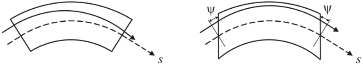
Figure 5:

Weak focusing in a sector dipole magnet (left) is a geometric effect resulting from the fact that two initially parallel trajectories (dashed and solid line) with equal bending radius approach and eventually cross each other because the outer arc is longer than the inner one. In a rectangular magnet (right), the trajectories do not approach each other because their arc length within the magnet is the same (and so is the bending angle). The pole-face angle ψ is defined with respect to the horizontal direction perpendicular to the beam.

In addition to the matrices for focusing and defocusing quadrupoles and drift spaces, there are two transfer matrices to describe a dipole magnet of length L. While a drift-space matrix is applied to the vertical plane, a focusing-quadrupole matrix in which |k(s)| was replaced by 1/R

²

(s) describes the focusing effect of a dipole in the (horizontal) bending plane. This replacement is motivated by the horizontal Eq. 12, and the resulting ”weak focusing” effect is explained in the caption of Fig. 5. It holds for sector dipole magnets with pole faces perpendicular to the beam. For a pole-face angle ψ 6= 0 (e.g. a rectangular magnet, for which 2ψ is equal to the bending angle Θ = L/R), the edge-focusing matrix M

_BE

must be applied for each edge. For the matrix element ± tan ψ/R, the positive sign holds for the (horizontal) bending plane and the negative sign for the other plane. The total transfer matrix of a dipole magnet is thus given by

M

_total

= M

_BE

· M

_B

· M

_BE

. (19)

For the case of a rectangular magnet, this can be shown to result in a drift-space matrix for the horizontal plane (i.e. weak and edge focusing cancel each other), while a vertically defocusing Lorentz force due to edge effects remains.

3.4.3 Optical functions

Apart from solving Eq. 12 in a piecewise fashion using transfer matrices, a general solution is given by

x(s) =

q

ε

x

β

x

(s) cos µ

x

(s), (20)

where ε

x

is a constant known as Courant-Snyder invariant, β

x

(s) is called the beta function

and µ

_x

(s) is the phase advance of the oscillation. Here and in the following, everything said for

the horizontal coordinate x applies to the vertical plane as well.

(14)

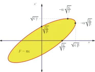
Figure 6:

Ellipse in horizontal phase space (positionxversus angular coordinatex⁰), parameterized by the optical functions (or ”Twiss parameters”)β_x,α_x≡ −β_x⁰/2 andγ_x≡(1 +α²_x)/β_x, which are functions of the positionsalong the machine while the ellipse area πε_x is the same everywhere. At a beam waist or bulge, the ellipse is upright withα_x= 0 andγ_x= 1/β_x(the subscripts x are omitted in the figure).

The beta function β

_x

(s) and its derivative, usually expressed by α

_x

(s) ≡ −β

_x⁰

(s)/2, can be calculated for a given lattice. Together with the the abbreviation γ

x

(s) ≡ 1 + α

²_x

(s)

/β

x

(s), they are referred to as optical functions

³

(or sometimes ”Twiss parameters”), and the locus of particles with the same ε

_x

is given by

ε

x

= γ

x

(s) x

²

(s) + 2α

x

(s) x(s) x

⁰

(s) + β

x

(s) x

⁰²

(s) , (21) which is a tilted ellipse in phase space (see Fig. 6). Here,

^p

ε

_x

β

_x

(s) is the a maximum spatial extension,

^p

ε

_x

γ

_x

(s) is the maximum angle, and πε

_x

is the area enclosed by the ellipse. Figure 7 shows a beam waist within a drift space as a simple example. While ε

x

is a constant property of each particle, the shape of the ellipse, on which the particle is found, depends on the position s along the machine and is given by the optical functions. For a large beta function, the ellipse is elongated in space and small in angle, and vice versa for small β

x

(s). For α

x

(s) = 0, the ellipse is upright and the ensemble of trajectories with varying ε

x

and random phase µ

x

forms a beam waist or bulge. Particles with different values of ε

_x

are on different concentric ellipses, and the

3 The derivation is beyond the scope of this text. Generally speaking, the optical functions form a vector (βx(s), αx(s), γx(s)), which can be transformed from one positions1 to another position s2 by a 3×3 matrix, which is constructed from elements of the transfer matrices. In a circular machine, the optical functions at one position can be found by using a periodicity argument (their values are the same after one turn), and once the optical functions are known at one position, they can be calculated for the whole machine. A similar procedure is used to determine the so-called dispersion functionDx(s) and its derivativeD_x⁰(s).

(15)

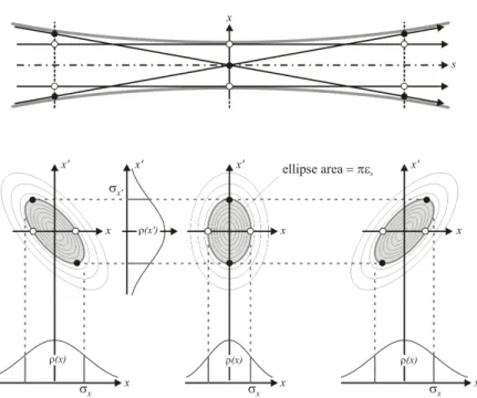
Figure 7:

Top view (xversuss) of a beam waist in a drift space, i.e. no magnetic field, with four particles on the same phase space ellipse: two with maximum offset (white dots), two with maximum angle (black dots). The trajectories of all particles on or within that ellipse lie within the envelope indicated by gray lines. The phase space distribution of a Gaussian beam is shown for three positions. The gray ellipses mark one standard deviation of xand x⁰. Their area has a constant value defined by πε_x, where ε_x is the horizontal beam emittance.

position of a particle on its respective ellipse is given by the phase µ

x

.

Since the number of betatron periods Q

_x

per turn, the so-called betatron tune, is necessarily a fixed number (of the order of 10), a simplified transfer matrix can be written for one turn around a circular machine

M

_{1 turn}

= cos 2πQ

x

β

x

sin 2πQ

x

−

_β¹

x

sin 2πQ

_x

cos 2πQ

_x

,

!

(22)

which depends on the beta function β

x

of the respective position and for α

x

= 0, i.e. a position

with a beam waist or bulge (there are additional terms for α

_x

6= 0 which shall be ignored for

simplicity). The deviation of the true magnetic fields from the idealized model can be described

by the ideal trajectory plus ”kicks” (small changes of x

⁰

) which are of no consequence as long

as they modify the trajectory turn by turn at different phases. If, for example, Q

_x

would be an

integer, the kick at a particular position would always deflect the particle in the same direction

and it would be lost. This is called a resonance. The same is true for not too small integer

fractions, and the general condition for harmful resonances is

(16)

m Q

_x

+ n Q

_y

= p, (23) where m, n, p are small integers and |m| + |n| is called the order of the resonance, which is typically relevant up to the order of 5. In a tune diagram with the fractional parts of the horizontal and vertical tune as the two axes, resonances form lines from which the working point of a machine should be kept clear.

3.4.4 Momentum-dependent effects

So far, the particle beam was assumed to be ”monochromatic”, i.e. each particle with the design momentum p, while typical deviations from that value are of the order of 0.1%. This has a number of consequences:

• The momentum-dependence of the bending radius in a dipole magnet gives rise to a hor- izontal displacement x

_D

(s) = D(s) ∆p/p of a particle with momentum offset ∆p, where the so-called dispersion D(s) and its derivative D

⁰

(s) are additional functions required to fully describe the linear optics of an accelerator or storage ring.

• The dispersive orbit x

_D

(s) usually results in a slightly larger/smaller circumference L for positive/negative momentum deviation, which is described by the so-called momentum compaction factor α ≡ (∆L/L

0

)/(∆p/p) which is calculated by integrating (D(s)/R(s))ds(s) along the ring.

• Since the focusing of a quadrupole magnet depends on the particle momentum, the be- tatron tune changes. Particles with positive/negative momentum offset tend to have a lower/higher tune as described by the so-called chromaticity ξ

_x

= ∆Q

_x

/(∆p/p). This re- sults in a distribution around the nominal tunes, effectively reducing the margin between harmful resonances. The chromaticity is obtained by integrating k(s)β

x

(s)ds along the ring.

The momentum dependence of the quadrupole focusing strength is reduced by sextupole magnets in a position with non-zero dispersion. Think of a quadrupole as a position-dependent dipole magnet and of a sextupole as a position-dependent quadrupole magnet. With a sextupole at a position with D(s) 6= 0, there is a correlation between momentum and transverse coordinate, and thus with focusing strength, such that particles with higher momentum are focused by a larger magnetic-field gradient.

With their magnetic field being nonlinear in x and y, sextupole magnets couple horizontal

and vertical motion and can give rise to chaotic trajectories for particles venturing beyond the

so-called dynamic aperture (in analogy to the physical aperture, given by solid obstacles such as

the vacuum chamber wall). There is no transfer matrix for sextupoles. Instead, their influence

on a particle can be approximated by kicks ∆x

⁰

and ∆y

⁰

, which depend on the sextupole strength

and on the particle position in x and y.

(17)

3.4.5 From single particles to particle beams

Often, a particle beam can be assumed to be Gaussian in all phase space coordinates. Consider- ing the phase space ellipse of a hypothetical particle at exactly one standard deviation in space and angle, the constant ε

_x

corresponding to that particle is called the horizontal emittance

⁴

of the beam. In hadron rings and in linacs, the emittance is given by how the beam is injected.

In electron storage rings, the horizontal emittance (typically a few rad m) results from an equi- librium between excitation due to the random nature of synchrotron radiation emission and a radiation damping effect. The vertical emittance in electron storage rings is mainly given by coupling due to field errors and misaligned magnets. A ratio between vertical and horizontal emittance of 0.01 to 0.001 can be achieved.

3.5 Outlook

This introduction to basic concepts of accelerator physics does by no means cover the topic exhaustively. As an outlook, two important items shall be mentioned briefly.

3.5.1 Beam diagnostics

No accelerator facility would operate successfully without extensive beam diagnostics and feed- back – either manual or automated – on parameters that deviate from their optimum values.

The diagnostics task includes:

• basic quantities such as beam energy, current, and lifetime (in storage rings),

• longitudinal position of bunches and transverse orbit position,

• distribution of the quantities mentioned above: beam size, bunch length, energy spread,

• optical functions: beta functions, dispersion, and their derivatives with respect to s,

• parameters like betatron tunes, momentum compaction factor, chromaticity, etc.,

• indications of external vibrations or intrinsic beam instabilities,

• technical parameters such as RF power and frequency, magnet currents etc.

4Unfortunately, it is common practice to use the same symbolεfor the Courant-Snyder invariant (which is a property of a single particle) and for the beam emittance (which is a property of the whole ensemble of particles).

Sometimes, the Courant-Synder invariant is called ”one-particle emittance” which is permissible if you understand the difference to the beam emittance, although some accelerator experts react with indignation to such sloppy language.

(18)

Figure 8: Order-of-magnitude frequencies in storage rings. RF systems operate typically at 300 to 500 MHz, revolution frequencies (1/turn) range from 11 kHz (at the LHC) to several MHz.

The frequencies for horizontal and vertical motion are slightly different, usually around 10 MHz, while longitudinal oscillations are three orders of magnitude slower. Not shown are harmonics and sidebands occurring in the beam spectrum.

A description of the methods to measure these quantities and, if required, to correct them is beyond the scope of this text (see e.g. [9]). With every generation of particle accelerators, inven- tive and more precise methods are devised. Furthermore, it must be remembered that particle accelerators are usually not directly accessible due to the radiation hazard, and a sophisticated control system is required to perform the formidable task of remotely detecting and controlling thousands of machine parameters.

3.5.2 Beam spectrum and collective effects

Since many phenomena in particle accelerators and particularly in storage rings are periodic, much can be learned from the beam spectrum measured by a pickup electrode at some position of the machine. Figure 8 shows typical frequencies, ranging from diurnal thermal variations to the RF frequency. Of particular interest is the horizontal and vertical betatron oscillation frequency, which shows the fractional part of the respective betatron tune, and the synchrotron oscillation frequency. Strong lines at these frequencies indicate the occurrence of beam instabilities.

Collective effects [10] are phenomena in which the motion of particles is not only determined by external fields (magnetic fields and the electric RF field) but by the presence of other beam particles. Electromagnetic fields trailing each particle bunch (so-called wake fields [11]) cause a coupling between bunches which may lead to collective multibunch instabilities [12]. In the case of a so-called longitudinal/transverse instability, particle bunches perform unwanted syn- chrotron/betatron oscillations. These oscillations degrade the beam quality and may even lead to beam loss. Another example of a collective effect is the scattering between beam particles within the same particle bunch which reduces the lifetime of a stored beam.

It happened several times in the history of accelerator physics that a new machine pushing the

limits of beam energy or current showed a new type of instability which first came as a surprise

and prevented the success of the project, but was subsequently studied, explained theoretically

and – if possible – cured (one example is the transverse PETRA instability [13]).

(19)

Instruments of Modern Physics – A Primer to Lasers, Accelerators, Detectors and all that