Purity Germanium Detectors

Analysis of Potassium induced Radioactivity in Chocolates based on γ Spectra taken with High

Purity Germanium Detectors

Analyse der kaliuminduzierten Radioaktivit¨at in Schokoladen basierend auf mit Hochreinen Germanium Detektoren aufgenommenen γ-Spektren

Technische Universit¨at M¨unchen

Bachelor Thesis

by

Martin Schuster

4. August 2014

Max-Planck-Institut f¨ur Physik

Werner-Heisenberg-Institut

Contents

1 Introduction 2

1.1 Potassium . . . . 2

1.2 Motivation . . . . 2

1.3 Structure of the Thesis . . . . 3

2 Experimental Setup 3 2.1 E ff ect of Shielding . . . . 5

2.2 Sample Preparation . . . . 6

2.3 Maximizing Statistic . . . . 6

2.3.1 Geometrical Acceptance . . . . 8

2.3.2 Choice of Container . . . . 10

3 Data Taking 11 4 Data Analysis 14 4.1 Calibration . . . . 14

4.2 Determination of the Counts in a Peak . . . . 15

4.3 Potassium Content . . . . 17

5 Results 17 5.1 Cacao content . . . . 17

5.2 Chocolates from Di ff erent Countries . . . . 19

6 Summary 22

1 Introduction

In this thesis the results of a study of the γ ray spectra for di ff erent kinds of chocolates are presented. The main source of natural radioactivity in chocolates is the potassium in cacao. Other elements contribute dependent on the country of origin. They are, for example, connected to geological conditions.

1.1 Potassium

Potassium is an important mineral which serves many purposes in the human body, such as the regulation of the fluid balance, protein synthesis, muscle contraction, synthesis of nucleic acids and control of the heartbeat. It can be found in many kinds of food and is thus consumed on a daily basis. Chocolates are especially rich in potassium, which is mainly contained in cacao [1].

There are three natural isotopes of potassium,

K,

K and

K. The only radioactive one is

K which has a natural abundance of 0.012%. It is one of the isotopes which undergoes all three forms of beta decay [2]. Figure 1 shows the decay schemata.

• About 89.28% of the time, β

-decay occurs. A neutron decays into a proton, an electron, e

, and an electron antineutrino, ¯ ν. This results in the decay of

K into the ground state of

Ca:

40

19

K →

Ca + e

+ ν . ¯

• In 10.72% of the cases, electron capture occurs. An electron from the K electron shell is captured in the nucleus. It is absorbed by a proton, p

, to form a neutron and an electron neutrino, ν is emitted. The

K becomes

Ar

with an electron missing in the K shell. The star * indicates that this is an excited state.

Ar

emits a characteristic 1460 keV γ-quant to go to the ground state

40

19

K + e

→

Ar

+ ν ,

40

18

Ar

→

Ar + γ (1460 keV) .

This decay facilitates the use of γ-spectroscopy to investigate the potassium content of samples.

A quantitative answer is possible as long as the potassium content is high enough to be detectable over the environmental background.

• Very rarely, about 0.001% of the time, β

decay occurs. A proton becomes a neutron under emis- sion of a positron, e

, and a ν. In this case

K goes directly into the ground state of

Ar.

40

19

K →

Ar + e

+ ν .

The response of the detector to a calibration source, see section 4.3, is used to deduce the potassium content of the source from the event count in the 1460 keV peak.

1.2 Motivation

The goals for this thesis were to investigate the potassium content of di ff erent chocolates and compare

them to the values that would be expected. Furthermore, since the amount of potassium should mainly

depend on the chocolates’ cacao content, chocolate with di ff erent cacao contents were compared to in-

vestigate the correlation. Additionally, chocolate from di ff erent countries having the same cacao content

were tested. Due to the respective soils the cacao grew on, or variations in the manufacturing process the

potassium content of the cacao might be di ff erent. For the same reasons ,other lines in the spectra might

be characteristic for the place of origin and were investigated.

(a) The possible decays of

K to

Ar are illustrated in this scheme.

(b) Here also the decay of

K to

Ca is taken into account.

Figure 1: Decay schemata for

K [2].

1.3 Structure of the Thesis

In chapter 2, the experimental setup is presented and the basics of spectroscopy with semiconductor detectors are explained. Some emphasis is put on count optimization as well as sample preparation. In chapter 3, an overview over the data taken is given. In chapter 4, the analysis is described in some detail before the results are presented and interpreted in chapter 5. The thesis ends with a summary in chapter 6.

2 Experimental Setup

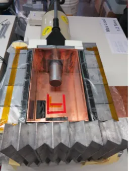
The experimental setup is shown in Fig. 2. A germanium detector is surrounded by a lead and copper shield with enough space even for large samples. The detector used is a Reverse Electrode Coaxial Germanium Detector (REGe), a high purity germanium detector produced by Canberra. The setup as a whole includes the following components:

Figure 2: View into the lead castle. The

lid is open. In the center the detector is

seen. The LN-dewar is outside the cas-

tle in the rear. The markings on the cop-

per serve consistent positioning of the

samples.

• In the center, the actual detector is enclosed in its vacuum cryostat, which is necessary to keep the temperature of the detector always around 100 K. Due to the small band gap value of germanium, the low temperature is needed in order to suppress the thermal generation of charge carriers [4].

The vacuum chamber also protects the sensible detector surfaces from contamination and moisture.

• A cooling finger reaches from the detector into its dewar. The dewar contains liquid nitrogen, LN, which has a temperature of roughly 77 K. It must be refilled regularly.

• The HV

-Generator provides a voltage, U

, of −4500 V. This voltage is applied in order to de- plete the detector from charge carriers. The electric field also helps to collect the photon-induced electrons and holes.

• In order to minimize the environmental background in the measured spectra, the detector is placed in a copper box which is surrounded by a lead castle during data taking. Due to its high atomic number and density, lead is a good choice of material to shield against γ-radiation.

• The DAQ system is a PIXIE-4 system from the company XIA. A Multi Channel Analyzer, MCA, is integrated [3].

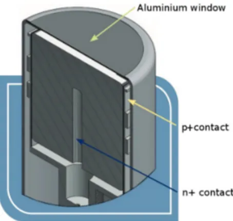
(a) The output signal of the semiconductor detector, REGe, is amplified, shaped and digitized (ADC). The data can now be processed with a PC.

(b) View into a REGe detector. Instead of the carbon composite window, an alu- minium window is used.

Figure 3: Schematics of the the pulse processing and the detector.

The principle of all semiconductor detectors is the same. Incident photons with a sufficiently high energy induce free electrons and holes through photo e ff ect, Compton scattering or pair production. The number of charge carriers is proportional to the energy deposited. By applying an electric field, these charge carriers are collected. The resulting electric pulses are digitized and recorded as indicated in Fig. 3a. The advantages over gas detectors are the much lower energy thresholds and a better energy resolution. The high speed of the charge carriers provides a good time resolution and the relatively high density of solids allows for good containment of the initial photons.

High purity germanium detectors rely on extreme purification of the material. Usually, there are around 10

electrically active impurities per cm

. They find their use predominantly in γ-spectroscopy.

They are able to distinguish γ lines ranging from few keV to several MeV. This is because they can be built with thin entrance windows and with a sensitive thickness of several centimeters. According

1

High Voltage

to the manufacturer, the detector used for the measurements presented in this thesis, the REGe, has a spectroscopy range from 3 keV to ≈ 10 MeV [4]. The lower limit is a result of the aluminium window, the upper a result of its size. A schematic of the detector is shown in Fig. 3b.

2.1 E ff ect of Shielding

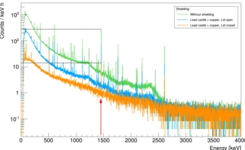
Chocolates are expected to be rather weak sources. Therefore it is especially important to minimize the background radiation. The impact of the lead and copper shields on the background is demonstrated in Fig. 4. The environmental background was measured without any shield, with only the lid o ff and with the lid on, see Fig. 5.

Figure 4: Environmental background spectra taken with di ff erent shielding. The Y-Axis is set to a logarithmic scale.

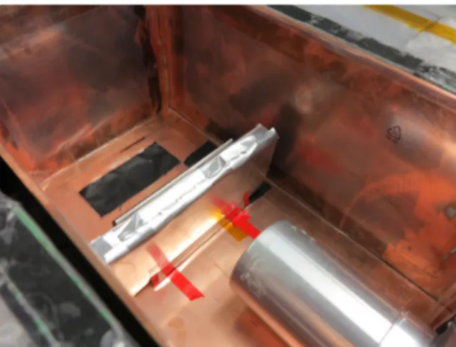
(a) Position of the detector is shown for the measurement without shields...

(b) with the lid taken o

... (c) and with closed shields.

Figure 5: Detector setups for the environmental background measurements.

The closed shield reduces the environmental background at 1460 keV by a factor of 20. This allows the study of this peak even for weak sources.

2.2 Sample Preparation

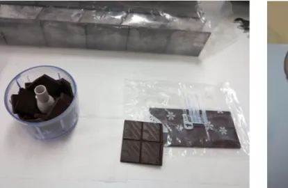
Since the bars of di ff erent brands of chocolate have di ff erent dimensions, the chocolate bars were chopped in order to obtain comparable results. The chopped samples were all measured inside the same container, which was cleaned diligently after each measurement. The chopper also was cleaned after each chop- ping. It was investigated whether chopping the chocolate impacts the results. In order to obtain su ffi cient

(a) The foil container next to its support. The thick aluminum foil was cut with the tools shown. The aluminum tape was used to seal the container. The red marking tape serves con- sistent positioning. The chocolate, still in its envelope, is shown in the left of the picture.

(b) View into the lead castle. The support fixes the foil con- tainer in a vertical position. This increases the surface fac- ing the detector and as a consequence the geometrical accep- tance, see

Figure 6: (a) Preparation and (b) setup for the measurement to investigate the impact of chopping the chocolate.

counts, three bars of the same kind of chocolate were used at once for this measurement. In order to maintain the same geometrical acceptance, see section 2.3.1, for chopped and unchopped samples, thick aluminum foil was wrapped tightly around the bare chocolate bars and formed to a container. In order to maximize the surface facing the detector, a support to hold the foil container in a vertical position was built, see Fig. 6. Measurements of the chocolate bars and the chopped chocolate, both using the same foil container, were performed. The background measurement is shared. The chopped chocolate did not fit completely into the container, thus its density is lower. The chopping was performed with an electric chopper from Tefal, see Fig. 7.

The results, after processing the data as described in section 4.2, are shown in Fig. 8. Since the values lie well within the margin of uncertainties, they can be regarded as equal and the e ff ect of chopping the chocolate is neglected for the subsequent sections.

2.3 Maximizing Statistic

The count rate recorded in the detector was maximized for the setup. The standard deviation, σ, on a number of observed counts, N, is √

N and increases with higher counts. The relative uncertainty,

(a) The chocolate is broken in to smaller pieces to fit in the chopper. (b) The chopper with the chopped chocolate inside.

Figure 7: The chopping process.

Figure 8: The amount of counts obtained in the 1460 keV peak per hour and kilogram for the three chocolate bars and the chopped chocolate. The graph shows that both values lie well within each others uncertainties. The line marks the average of the values.

however, improves [5].

σ N =

√ N N = 1

√

N (1)

The observed number N depends on

• the activity of the source, which anon depends on the material and the mass

• the measuring time

• the acceptance, e.g. the ratio of recorded counts over emitted gammas. The acceptance is dom- inated by geometrical effects, because self absorption in the samples is below 5% [6]. The self absorption thus is neglected in the current analysis.

2.3.1 Geometrical Acceptance

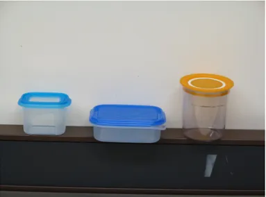
Due to the isotropic nature of the emitted radiation, the amount of photons recorded in the detector does depend on its physical position relative to the detector. The distance to the detector, as well as the surface facing the detector or the relative height of the source all have an influence. Different containers at di ff erent distances were studied. The containers are shown in Fig. 9.

Figure 9: The available containers that were be evaluated. The small blue box, the blue box and the yellow box.

Assuming a point-like source at a radial distance from the detector, r

, and given the cylindrical shape of the detector with r

= 35 mm the geometrical acceptance,

, can be estimated as the ratio of the surface of the window of the detector S

and the spherical surface S

of the isotropic radiation.

= S

S

= π · r

4π · r

(2)

The estimated geometrical acceptances for the different containers derived with Eq. 2 are given in Table 1. This calculation neglects the real geometry of the containers as well as the acceptance for gam- mas entering the detector from the side. In addition, it does not take into account the probability that a interacting gamma is fully contained.

To determine the true acceptance,

, a calibration source was used. Each container was filled with potassium chloride, KCl, as the calibration source. The specific properties of KCl are given in Table 2.

For a given mass of KCl, m

, the respective activity, A, was calculated as

A = m

· (1 − i

) · m

· a

m

K

· N

· ln(2) t

2

· BR

, (3)

Container Distance to the detectorrS[mm] Geometrical acceptanceest[%]

Small blue box 72 6

Blue box 48 13

Yellow box 92 4

Yellow box near 77 5

Table 1: Approximated geometrical acceptances for the different containers using Eq. 2. The distances are given from the respective centers of the containers.

Impurity content i

=0.258 %

Molecular mass contribution from the Potassium m

= 52.45 % Natural isotopic abundance of

K a

= 0.012%

BR of the

K in

Ar by β

and isomeric transition BR

= 10.67 %

Half Life of

K t

2

= 1.2483 · 10

years Table 2: Relevant values given by the KCl manufacturer [7] and the Half Life [2].

where m

K

is the atomic mass and has a value of 39.96

. The measured e ffi ciency is obtained as

= C

A (4)

where C

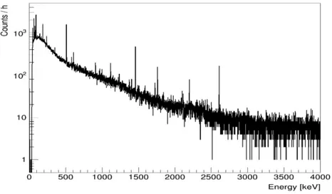
is the normalized count rate observed. For this particular study, not only the full absorption peak at 1460 keV, but also the Compton continuum was used. The single escape peak at 949 keV and the double escape peak at 438 keV were also included. The number of photons recorded in the detector was determined by evaluating the integral from zero to 1466 keV after the environmental background, see Fig. 10, was subtracted.

Figure 10: An example background measurement with a lifetime of 40.06 hours.

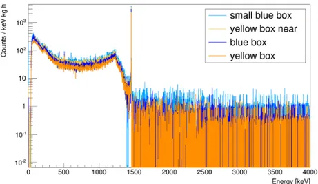
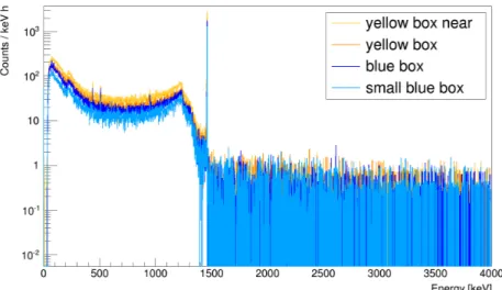
Figure 11 shows the background subtracted spectra for the di ff erent containers. The small blue box

provides the most counts per mass and time compared to the others. In Table 3, the count rates C

and

e ffi ciencies,

, for the four configurations are listed. The small blue box provides the best geometrical

acceptance. The values for

show that the simplistic approach, on which the estimates given in Table 1

were based, is not adequate here.

Figure 11: Spectra normalized to mass and lifetime of the measurements. The small blue box provides the most counts per hour and kilogram.

2.3.2 Choice of Container

Even though the yellow container in the near position did not provide the best

, it was chosen for the measurements. While in most cases and in absence of other e ff ects the setup providing the best geometrical acceptance is preferable, the actual goal is to maximize the counts N per time. Since the containers differ significantly in their volume, in this case the best geometrical acceptance does not mean the most counts per time. As can be seen from Table 3 and figure 12, due to its larger volume, the yellow box in the near position provides the best performance.

Container m

[g] A [Bq] C

[s

]

[%]

Small blue box 345.3 613.53 10.21 1.66

Blue box 597.0 1060.76 14.53 1.37

Yellow box 851.5 1512.96 16.73 1.11

Yellow box near 817.5 1452.54 22.96 1.58

Table 3: Count rates and geometrical acceptances for four measurement configurations.

Figure 12: Spectra scaled for the lifetime for four measurement configurations. The KCl in the yellow box at the near position provides the highest count rate.

3 Data Taking

In this section an overview over all the measurements is given. The data acquisition system, DAQ, has an interface from which its steering parameters are set. In Table 4, the settings for the data taking are listed.

Type of measurement

time & energy only

Threshold

20

Gain

3

Trigger share mode

0

Good Channel

Read always Enable trigger Histogram Energies

Table 4: DAQ settings for all measurements.

Tables 5 - 9 list all measurements. The lifetime of a given measurement was provided by the DAQ.

The sample masses were measured with a precision balance, PCB, from KERN. A measurement of

the environmental background was associated with each sample measurement. The lifetime of these

background measurements was at least four times as long as the one of the respective sources. Since

the container does not change for entire series of measurements, an overnight measured environmental

background can be assigned to measurements from the day before and after. Thus several measurements

share the same background measurement.

Label State Date Livetime [days] Mass [g] Background, see Table 9

S1

Chocolate bars 20 July 0.124897 306.8

B

S2

Chopped chocolate 21 July 0.152446 280.7

Table 5: The chocolate was first measured in bars and then chopped.The foil container used can be seen in Fig. 6.

Label Container Date Lifetime [days] Mass [g] Background, see Table 9

S1

Yellow box 6 May 0.0903148 851.5 B1

S2

Small blue box 8 May 0.0799803 345.3 B2

S3

Blue box 8 May 0.1023260 597 B3

S4

Yellow box near 13 May 0.0901231 817.5 B4

Table 6: Measurements of KCl to support the choice of container. The containers used are shown in Fig. 9.

Label Cacao [%] Date Lifetime [days] Mass [g] Background, see Table 9

S1

90 13 May 0.109573 429.9

B1

S2

85 15 May 0.145525 430.8

S3

50 22 May 0.167698 450.2 B2

S4

70 2 June 0.158033 499.3 B3

Table 7: The measured chocolates with their respective percentages of cacao as given by the manufac- turer Lindt.

Label Country of origin Date Lifetime [days] Mass [g] Background, see Table 9

S1

Chuao (Venezuela) 5 June 0.150137 450.7

B1

S2

Puerto Cabello (Venezuela) 5 June 0.158033 451.7

S3

Trinidad and Tobago 6 June 0.157173 462.2

S4

Sri Lanka 9 June 0.153659 471.5

B2

S5

Madagascar 9 June 0.153073 469.0

S6

Equateur 10 June 0.152544 470.8

S7

Cote d’Ivoire 10 June 0.151795 466.0

B3

S8

Hacienda El Rosario (Venezuela) 11 June 0.154520 466.5

Table 8: The international chocolates with their country of origin. The cacao percentage for all of them

is given as 75 % and the manufacturer is Chocolat Bonnat.

Label Date Lifetime B

20 − 21 July 0.531838 B1

6 − 7 May 1.665475 B2

9 − 10 May 1.053045 B3

10 − 12 May 1.723672 B4

13 − 15 May 1.668974 B1

13 − 15 May 1.668974 B2

22 − 26 May 3.63569 B2

2 − 5 June 2.630273 B1

5 − 6 June 0.618057 B2

9 − 10 June 0.612951 B3

10 − 11 June 0.623746

Table 9: Summary of all measurements for environmental plus respective container background.

4 Data Analysis

In this chapter, the steps to deduce the potassium content from the measured spectra are described.

4.1 Calibration

The data have to be calibrated in order to translate the channel numbers from the DAQ into energies.

Figure 13a shows a raw spectrum in channel numbers. The peak around channel number 12070 was identified as the

K peak. Figure 13b shows a Gaussian fit to this peak of 1460 keV. The mean of the fit corresponds to the known energy of 1460 keV. Additional peaks used were the 511 keV peak from electron positron annihilation

and the 2614 keV peak from

Tl decay [8]. Figure 13c shows the corresponding calibration points plus a linear fit. The fit parameter p0 is compatible with 0, confirming the linearity of the system. The fit parameter p1 is the calibration constant which is determined to better than one per mille. Figure 13d shows the calibrated spectrum. The bin width is increased compared to 13a.

(a) Raw spectrum of measurement B4

. (b) Fit of the 1460 keV peak.

(c) Calibration points at 511 keV, 1460 keV and 2614 keV respectively. The linear fit was used as final calibration.

(d) Final spectrum after the calibration process

Figure 13: Illustration of the calibration process for background measurement B4

, see Table 9.

2

An initial photon interacts with

pair creation and the

annihilates

4.2 Determination of the Counts in a Peak

To determine the counts in a peak, the peak is fitted and the fit function is integrated. The fit function for a γ-ray peak is not a simple Gaussian. Several e ff ects have to be taken into account [9][10][11]:

• For a γ-ray line with a negligible natural width, a sharp Gaussian peak broadened by statistical and electronics noise is expected 5.

• When the charge collection is incomplete or pile-up occurs, counts may be removed from the sharp peak. This leads to an exponentially decaying distribution under the peak, i.e. a skew plus shoulder on the low energy side of the Gaussian 6.

• The peaks studied are full absorption peaks. Compton Scattering enhances the background below the peak compared to above. This adds a smeared step function 7.

• The Compton continuum from higher energy gamma peaks is usually well represented by a first order polynomial.

The fit function used to cover the e ff ects is

F(X, σ, b, A, F

, I) = A · (1 − F

)

2π

exp −

2σ

!

(5) + A · F

X b+₂^σ_b²2

1−erf

√X

2σ+^√₂^s_b

2b

(6)

+ I · 0.5 erfc

√X 2s

(7) Here, σ is the standard deviation and A is the area underneath the peak. X equals x − µ, with µ being the center of the fit. The parameter b equals W

· σ with W

being the skew width and F

is the skew fraction. Finally I is the step amplitude. The linear function representing the background does not contribute to the actual shape of the peak and thus is treated separately. All the parameters are obtained by the fitter. For especially low count rates, in some cases the skew was turned off

, or a polynomial of degree zero was used to represent the background continuum. This was necessary to have a stable fit.

The fits were performed using the software package ROOT. The fitter used is based on the Maximum Likelihood method. Maximum Likelihood is a statistical approach that, instead of assessing the proba- bility density for any values x

... x

for a fixed parameter q, regards the density as a function of q for observed and thus fixed appearances of x

... x

. This leads to the Likelihood-Function [12][13][14]

L(q) =

n

Y

i=1

f

(x

; q) . (8)

Maximizing this function in dependence of q leads to the Maximum Likelihood estimate for q. Basically the value for q is searched, for which the sample values x

... x

have the highest probability density.

The fits were always done to calibrated, but otherwise raw spectra. The obtained values of A and thus the count rates in the peaks with their uncertainties are results of the fit. After scaling for the lifetime, A is divided by the relevant bin width and represents a count rate. Rates are determined for the sample measurement, C

, and the corresponding environmental background, C

. Figure 14 shows the

3

Term

was not taken into account in F(X,

,

(a) Fit to the calibrated signal plus background spectrum. (b) Fit to the calibrated spectrum for the environmental back- ground measurement.

Figure 14: Fit to the calibrated 1460 keV peaks for measurement S3

and the corresponding envi- ronmental background B1

. The number of counts in the peak plus uncertainties are obtained by ROOT. The fit function is composite of a Gaussian plus skew, a step and a linear function [9][10][11].

Label C

h

h

i ∆ C

h

h

i

S1

18.507 5.278

S2

19.714 5.325

S1

119.082 7.667

S2

104.820 6.319

S3

29.119 4.282

S4

54.944 4.850

S1

42.117 4.874

S2

50.589 5.009

S3

43.318 4.845

S4

44.595 4.811

S5

49.405 4.946

S6

55.023 5.183

S7

45.931 5.283

S8

43.931 4.764

S4

6953.49 56.940

Table 10: The obtained count rates with uncertainties. The mass of the samples is not yet taken into consideration.

result of the fits for the 1460 keV peak of measurements S3

and B1

, see Tables 8, 9. After the scaling, the count rates from the background are subtracted the following way [5] :

C

= C

− C

, (9)

∆ C

= r

∆ C

+

∆ C

. (10)

C

is the number of counts per time that originate from the sample with the mass m

. Table 10 lists

the C

for all the relevant measurements with the respective uncertainties.

4.3 Potassium Content

To deduce the content of potassium from the count rates, they are calibrated with KCl, see chapter 2.3.1.

With knowledge of the exact amount of potassium, m

(KCl), and the corresponding count rate under- neath the 1460 keV peak, C

, the amount of potassium in any source, m

(src), can be deduced by measuring its corresponding count rate, C

. The calibration equation is

m

( src) = C

C

m

(KCl) . (11)

The mass of potassium in the KCl salt, m

(KCl), can be derived by the following equation:

m

(KCl) = (1 − i

) · m

· m

, (12) with the quantities as described in Table 2. The uncertainty for i

is estimated to be 0.1 %, the precision of the scale for m

is 0.2 g, and the uncertainty of m

, ∆ m

, is assumed to be zero. The treatment of the uncertainties as a first order approximation can be performed like this [5]

∆ m

(KCl)

|m

(KCl)| = v t

∆ i

1 − i

!

+



 

 



∆ m

m



 

 



2

+ ∆ m

m

!

. (13)

Solving for ∆ m

(KCl) leads to

∆ m

(KCl) = v u t

(1 − i

) · m

· m

·



 

 

 



∆ i

1 − i

!

+



 

 



∆ m

m



 

 



2

+ ∆ m

m

!



 

 

 



. (14) In analogy to Eq. 14 the uncertainty for m

(src), see Eq. 11, can be written as

∆ m

(src) = v u u t

 

 

 

 C

C

m

(KCl)



 

 

 



2

·



 

 

 

 

∆ m

(KCl) m

(KCl)

!

+



 

 

 

∆ C

C



 

 

 

2

+



 

 

 



∆ C

C



 

 

 



2



 

 

 

 

. (15)

The uncertainties for the count rates are obtained like described in 4.2. The uncertainty ∆ m

(src) in- cludes all statistical and systematic e ff ects. It is dominated by the statistics of the count rate. It has been verified that the asymmetry on the uncertainties neglected in Eq. 15 is indeed negligible.

These calculations return the amount of potassium in grams that is contained in the source. In order to compare the results, it has yet to be scaled with the mass of the sample. Dividing m

( src) by the mass of the source, m

, delivers the percentage of potassium, K

, for the respective sources:

K

= m

(src)

m

, (16)

with

∆ K

= v t

m

(src) m

!

·



 

 

 

∆ m

(src) m

( src)

!

+ ∆ m

m

!



 

 

  . (17)

5 Results

5.1 Cacao content

Typically, cacao has a potassium content of 1524 mg per 100 g [15]. The potassium content, m

, in 100 g of chocolate with a listed cacao content, C

, can be estimated as:

m

= C

100 · 1.524 g . (18)

Percentage of cacao [%] Expected

K content [g] Measured

K content [g] Uncertainty [g]

50 0.762 0.397 0.058

70 1.066 0.676 0.060

85 1.295 1.496 0.091

90 1.371 1.703 0.110

Table 11: Overview on the expected and measured potassium contents for chocolates with different listed cacao percentages.

In Table 11, the expected and measured values for m

are listed. Figure 15 illustrates the data.

The measured and expected m

are of compatible magnitude. However, the measured values are incompatible with a simple linear dependency. The expected values only take the potassium from the cacao into account. In real chocolates, there are other ingredients which may, even if slightly, contribute to its total potassium content. However, for low percentages of cacao listed, the measured potassium content is lower than the expectation. This would rather indicate that some potassium was lost in the fabrication process. An extrapolation to zero % cacao roughly yields zero potassium. The influence of composites other than cacao seem to really have a minor impact on the potassium content.

Figure 15: The measured values alongside the expected ones for the potassium content

The values for 85 % and 90 % cacao content are clearly above expectation. The uncertainties are too large to determine a slope, but these chocolates are different from the low % chocolates. This discrepancy is surprising and indicates that either the cacao values given by the manufacturer are a significant source of uncertainty or the processing enriches or depletes the cacao of potassium. The manufacturers indeed do not claim, that the given percentages are correct, but that they are lower limits for the cacao content.

That could explain the measured values at 85 % and 90 %.

Location of origin Expected

K content [g] Measured

K content [g] Uncertainty [g]

Chuao 1.143 0.574 0.066

Hacienda el Rosario 1.143 0.579 0.063

Puerto Cabello 1.143 0.663 0.065

Trinidad and Tobago 1.143 0.576 0.064

Ecuador 1.143 0.718 0.068

Sri Lanka 1.143 0.581 0.062

Cote d’Ivoire 1.143 0.605 0.069

Madagascar 1.143 0.672 0.067

Table 12: Overview on the expected and measured potassium contents for the di ff erent locations of origin. The listed cacao percentage is 75 % for all of the chocolates.

5.2 Chocolates from Di ff erent Countries

The potassium content of chocolates from different countries was investigated. Since the cacao percent- age is listed as 75 % for all of them, similar values are expected. Figure 16 visualizes the results. The countries are grouped in three regions, northern South America in general, Venezuela in particular and the others, including Africa and Sri Lanka.

Figure 16: The potassium content of the chocolates for the di ff erent countries of origin. The color code indicates geographic regions.

Assuming equal cacao content and processing, the di ff erences in the potassium content stem from the soils the cacao plants grew on. No significant differences were observed. The potassium content in cacao seems to be the same everywhere.

Other than potassium, the plants incorporate many elements from the soils during growth. Some are radioactive and emit γ rays that show in the full spectra. It was investigated whether characteristic lines for some country of origin or even a certain region exist. The spectra were scaled for their lifetime and the respective environmental background was subtracted. Negative counts occur due to the statistical fluctuations. After the subtraction the spectra were scaled for the sample masses. The most relevant lines are listed in Table 13 [8].

Figure 17 shows the spectra of the chocolates from Africa and Asia. The di ff erences in the 1460 keV

γ Energy [keV] Source Alternate source

295.2 U-

Pb

351.9 U-

Pb

511 annihilation

609.3 U-

Bi

As

1120.5 U-

Bi(1120.3)

Ti

1460

K

1763 U-

Bi(1764.5)

Ti (1762.0)

2203 U-

Bi

2614.5 Th-

Tl

Table 13: Selection of γ energies [8] occurring in the spectra of the international chocolates.

peak are negligible, see Fig 16. The chocolate from Sri Lanka as opposed to the African chocolates shows an indication for

Bi across the board, see Table 13. This is especially visible for the 609.3 keV line. Additionally the 295.2 keV and 351.9 keV lines stemming from

Pb are very distinct. Both el- ements are part of Uranium decay chains. Those lines give evidence for enhanced Uranium content in the soil of Sri Lanka. The

Tl line is the strongest for the chocolate from Madagascar and indicates a slightly enhanced content in the soils there.

Figure 17: Comparison of the full spectra for the chocolates from Africa and Sri Lanka.

Figure 18 shows the spectra for the chocolates from Venezuela. The

Tl peak is enhanced for the chocolate from Puerto Cabello. It would indicate an increased Uranium content. The lower energy peaks are not significant due to the statistical fluctuation of the environmental background.

Both South American chocolates are shown in Figure 19. The most significant line is similar to Sri

Lanka the 609.3 keV

Bi line for Ecuador. The other

Bi lines are also indicated. The soils in

Ecuador seemingly also have an enhanced Uranium content.

Figure 18: Comparison of the full spectra for the chocolates from Venezuela.

Figure 19: Comparison of the full spectra for the chocolates from South America.

6 Summary

In this thesis, a procedure sensitive enough to perform γ spectroscopy on chocolates was described. The procedure was applied on different samples of chocolate to obtain the potassium content of the choco- late. The γ radiation mainly stems from the

K isotope and the potassium content can be deduced by analysing the associated 1460 keV peak. The correlation of the listed cacao percentage to the potassium content was investigated as well as other characteristics in the spectra for chocolates from different coun- tries of origin.

The experimental setup and the basic principle of spectroscopy with High Purity Germanium Detectors were described. The importance of shielding and sample preparation were demonstrated. For the pur- pose of maximizing the statistic several containers were investigated for their geometrical acceptances, and the one providing the most counts recorded in the detector was chosen. Data taking was described and all data sets listed. Emphasis was put on the description of the processing of the data, including calibration, fitting of the peaks and the extraction of the potassium content from the 1460 keV peak.

The results were presented and discussed. It was verified that the potassium content is related to the percentage of cacao. However, a linear dependence was only observed for low cacao % chocolate.

The full spectra were investigated to search for characteristic lines associated to the country of origin.

Evidence for an excess of

Bi and

Pb for chocolate from Sri Lanka and

Tl for the chocolate from

Puerto Cabello in Venezuela was found. Also some indication for an enhanced

Bi content for the

chocolate from Ecuador was observed.

References

[1] U. S. D. of Agriculture, http://ndb.nal.usda.gov/ndb/nutrients/index, checked typical chocolate in- gredients for potassium content.

[2] R. B. Firestone et al., Table of Isotopes (Wiley - Interscience, 1996), 8th ed.

[3] X. LLC, User’s Manual Digital Gamma Finder (DGF) Pixie-4, 31057 Genstar Road, HAyward,CA 94544 USA (2012).

[4] Germanium Detectors: User’s Manual, Canberra Industries,800 Research Parkway, Meriden, CT 06450 (2003).

[5] J. R. Taylor, AN INTRODUCTION TO Error Analysis (University Science Books, 1997), 2nd ed.

[6] L. Garbini, Personal conversation (2014).

[7] AppliChem, Potassium chloride pure Ph.Eur. (2014).

[8] L. G. Evans, R. C. Reedy, R. D. Starr, et al., Journal of Geophysical Research 111 (2007).

[9] G. W. Phillips and K. W. Marlow, Nuclear Instruments and methods 137, 525 (1976).

[10] J. Kern, Nuclear Intruments and methods 79, 233 (1970).

[11] L. McNelles and J. Campbell, Nuclear Intruments and methods 127, 73 (1975).

[12] J. Schwarze, Grundlagen der Statistik - Band 2: Wahrscheinlichkeitsrechnung und induktive Statis- tik (Herne Verlag, 1997), 6th ed.

[13] V. Blobel and E. Lohrmann, Statistische und numerische Methoden der Datenanalyse (Teubner Studienbcher, 1998).

[14] J. Felsenstein, Inferring Phylogenies (Sinauer Associates, 2003).

[15] U. S. D. of Agriculture, Basic Report: 19165, Cocoa, dry powder, unsweetened (2014).