Measurements of the photon identification e ffi ciency with the ATLAS detector using 4.9 fb

(1)

ATLAS-CONF-2012-123 17August2012

ATLAS NOTE

ATLAS-CONF-2012-123

August 13, 2012

Measurements of the photon identification e ffi ciency with the ATLAS detector using 4.9 fb

⁻¹

of pp collision data

collected in 2011

The ATLAS Collaboration

Abstract

The efficiency of the tight selection criteria used in the 2011 dataset by the ATLAS experiment to identify photons is measured using 4.9 fb⁻¹ of ppcollision data. Three independent data-driven methods are used to estimate the identification efficiency in different regions of pseudorapidityηand as a function of the photon transverse momentumE_Tin the 15−300 GeV range. The three measurements give consistent results, and are combined in the overlappingE_Tregions into a single data-driven efficiency map.

The comparison of this data-driven efficiency map with that predicted by the ATLAS simulation shows significant disagreements in some η andE_T regions, where the simulation systematically predicts higher photon identification efficiency values. A simple data- driven correction procedure, implemented by slightly shifting the simulated electromagnetic shower shapes, restores the agreement with the data-driven values within±5%.

c

Reproduction of this article or parts of it is allowed as specified in the CC-BY-3.0 license.

(2)

1 Introduction

Several physics processes produce final states with prompt photons in ppcollisions [1–4]. The study of such final states, and the measurement of their production cross sections, are of great interest at the LHC as a probe of perturbative QCD. At the same time, the prompt photon production represents an irreducible background for some new physics processes, such as the Higgs boson decay into photon pairs [5], or multi-photon production predicted as characteristic signatures of some exotic models of physics beyond the Standard Model [6, 7].

The identification of prompt photons in hadronic collisions is particularly challenging since the over- whelming majority of final state photons originate from neutral hadron decays or from radiative decays of other particles. Prompt photons are separated in the ATLAS experiment from these background photons by means of selections on quantities describing the shape and properties of the associated electromagnetic showers and by requiring them to be isolated from other particles in the event [8].

While an estimate of the efficiency ε_ID of the photon identification criteria can be obtained from Monte Carlo (MC) simulation, measuring it from data presents several difficulties. Unlike for electrons, whereJψ→ee,W→eνandZ →eedecays can be used [9], there are no physics processes that produce very clean samples of prompt photons in a large ET range. In this respect, the only process playing a similar role for photons is theZ → ``γradiative decay (` being an electron or a muon), that is very limited by the small production cross section and by its kinematics in itsE_Treach.

The ATLAS collaboration has traditionally evaluatedε_ID using MC simulated samples, corrected for the differences in the electromagnetic shower shapes observed between data and simulation. The uncertainty on these MC-basedε_IDvalues were mainly associated to the correction technique, that had to account for the imperfect knowledge of the material in front of the electromagnetic calorimeter, the uncertainty on the photon candidate purity, and the accuracy of the data/MC discrepancy parametrizations used to correct the MC.

In this document, the efforts to directly measure the photon identification efficiency using 2011 pp data are summarized and discussed. Three different data-driven techniques are used: selecting photons from radiative decays of theZboson; extrapolating photon properties from electrons and positrons from Zdecays by exploiting their similarity to photons; and implementing a technique to determine the fraction of background present in a sample of isolated photon candidates in the initial sample (“matrix” approach).

Each of these techniques can measureε_IDin complementaryE_Tregions with varying precision.

This document is organized as follows. In Section 2 a brief description of the photon identification in the ATLAS experiment is given. In Section 3 the three data-driven approaches to the measurement of the photon identification efficiency are described, listing their respective sources of uncertainty, and the precision they can reach in the relevantE_Tranges. The consistency of the results allows for a combination of the measurements into a single data-driven estimate, as shown in Section 4. In Section 5 their combination is compared to the MC predictions. Section 6 is devoted to the study of the impact of the photon identification efficiency on the number of collisions superimposed on the same bunch crossing (pileup).

The simulation of the detector response to pileup is evaluated by comparing to the measurements. Since all measurements discussed in Section 3 are performed for a given photon isolation requirement, Sec- tion 7 is devoted to investigating how the photon identification efficiency varies as a function of the isolation criteria, and to evaluate the impact of a potentially worse efficiency for the reconstruction of photon conversions. In Section 8 the results are summarized.

2 Photon identification in ATLAS

Photons are reconstructed by the ATLAS detector as isolated objects with most of their energy deposited in the electromagnetic calorimeter (EMC). The details of the reconstruction procedure, and the way the

(3)

ambiguity between converted photons and electrons is resolved, are described in detail in Ref. [8].

The ATLAS EMC [10] is a lead-liquid argon (Pb-LAr) sampling calorimeter with an accordion geometry. It is divided into a barrel section, covering the pseudorapidity region |η| < 1.475, and two end-cap sections, covering the pseudorapidity regions 1.375<|η|<3.2. It consists of three longitudinal layers: the first one, with a thickness between 3 and 5 radiation lengths, is segmented into high granularity strips in theηdirection (width between 0.003 and 0.006 depending onη, with the exception of the regions 1.4 < |η| < 1.5 and|η| > 2.4), sufficient to provide an event-by-event discrimination between single photon showers and two overlapping showers coming from aπ⁰ decay. The second EMC layer, which collects most of the energy deposited in the calorimeter by the photon shower, has a thickness around 17 radiation lengths and a granularity of 0.025×0.025 inη×φ(corresponding to one cell). Theη position of the photon candidates is measured from the energy-weighted barycentre of the cluster in the second layer of the EMC. A third EMC layer, with thickness varying between 4 and 15 radiation lengths, is used to correct leakage beyond the calorimeter for high energy showers.

2.1 Photon identification criteria

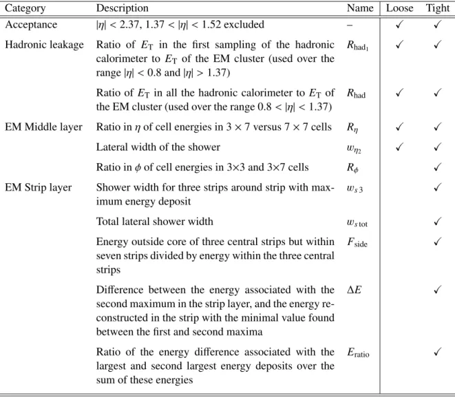
Prompt photons need to be separated from jets with a large electromagnetic component, mostly associated to the decay to photon pairs of neutral mesons in hadronic jets. The baseline ATLAS photon identification algorithm relies on rectangular cuts using calorimetric variables, defined using the energy deposit in the EMC cells. These discriminating variables (DV, listed in Table 1) are computed in the different EMC layers exploiting the fine cell granularity [8], and reflect the different shapes of the electromagnetic showers induced in the EMC by isolated photons and QCD jets.

A photon coming from the hard scattering can convert into ane⁺e⁻pair as it transverses the material in front of the EMC. The ATLAS Inner Detector (ID) tracking system is used to reconstruct conversion vertices up to a radius in the transverse plane (R) less than 80 cm, one of which can sometimes be associated to a photon cluster: in these cases, the photon candidate is referred to as aconvertedphoton.

Converted photons are further categorized into single and double-track conversions, depending on the number of reconstructed tracks.

Two reference sets of cuts – loose and tight – are defined. The loose selection is harmonized with the corresponding electron one, and used for triggering purposes. The tight selection is separately optimized for unconverted and converted photons to provide a photon identification efficiency of about 85% for photon candidates with transverse energyE_T>40 GeV, and a corresponding background rejection factor of about 5000 [8]. The cut-based selection criteria do not depend on the photon candidate transverse energyE_T, but vary as a function of the reconstructed pseudorapidityηof photon candidates, to take into account variations associated to the total thickness of material in front of the EMC and the calorimeter geometry.

During the 2010 and 2011 data taking, the loose and the tight selections documented in Ref. [8]

underwent minor changes aimed at reducing the systematic effects associated to the differences between the calorimetric variables measured from data and their description by the ATLAS simulation.

2.2 Photon isolation

An isolation requirement, based on the transverse energy deposited in the calorimeters in a cone around the photon candidate, is used to further suppress the main background from neutral hadrons decaying into two photons. The transverse isolation energyE^iso_T is computed using calorimeter cells from both the electromagnetic and hadronic calorimeters, in a cone of radiusRin theη−φspace around the photon candidate. This quantity is corrected for both energy leakage outside of the cone and for pileup effects, as described in Refs. [11] and [12].

(4)

Category Description Name Loose Tight Acceptance |η|<2.37, 1.37<|η|<1.52 excluded – X X Hadronic leakage Ratio of E_T in the first sampling of the hadronic

calorimeter to E_T of the EM cluster (used over the range|η|<0.8 and|η|>1.37)

R_had₁ X X

Ratio of E_T in all the hadronic calorimeter to E_T of the EM cluster (used over the range 0.8<|η|<1.37)

R_had X X

EM Middle layer Ratio inηof cell energies in 3×7 versus 7×7 cells R_η X X

Lateral width of the shower w_η₂ X X

Ratio inφof cell energies in 3×3 and 3×7 cells R_φ X EM Strip layer Shower width for three strips around strip with max-

imum energy deposit

ws3 X

Total lateral shower width wstot X

Energy outside core of three central strips but within seven strips divided by energy within the three central strips

F_side X

Difference between the energy associated with the second maximum in the strip layer, and the energy reconstructed in the strip with the minimal value found between the first and second maxima

∆E X

Ratio of the energy difference associated with the largest and second largest energy deposits over the sum of these energies

E_ratio X

Table 1: Variables used for loose and tight photon identification cuts.

2.3 Photon identification efficiency

Taking isolation into account, ε_ID(E_T, η) is defined as the efficiency for reconstructed prompt photons with measured E^iso_T < E^iso_T |_cutto pass the tight photon identification criteria in a givenE_T, ηregion. For reconstructed photons with reconstructed|η|in the pseudorapidity bink(with lower and upperηvalues ofηk,1andηk,2, respectively)ε_ID(E_T, η) can be expressed as:

ε_ID^k(E^γ_T,reco)≡

dN^γ(ηk,1≤ |η^γ_reco|< ηk,2,E^iso_T,reco<E^iso_T |_cutGeV,tight−ID)/dE^γ_T,reco

dN^γ(η_k,1≤ |η^γ_reco|< η_k,2,Eîso_T |_cutGeV)/dE^γ_T,reco (1) The chosen value of E_Tîso|_cut depends on the goals of each physics analysis, and the corresponding E_T range under study. It has evolved from 3 GeV used in 2010 analyses [1–4] to a widely-used value of 5 GeV adopted by most of the ATLAS photon analyses based on 2011 data [13]. Following the more common prescription used by the ATLAS photon analyses, a cone of radiusR=0.4 is used, and aEîso_T |_cut

=5 GeV cut is applied when computingε_IDvalues. Any residual dependence on the choice of a different photon isolation prescription is discussed in Section 7.2

(5)

3 Data–driven measurements of photon identification e ffi ciency

Three data-driven methods are used to measure the photon identification efficiencyε_IDcorresponding to the tight selection criteria described in Section 2.1.

• The first method relies on the use of a pure photon sample selected from the radiative decays of the Zboson, and allows a precise measurement in the lowE_Tregion. In this analysis, theZelectron- and muon-decay channels are initially treated independently. As the results of the two channels give consistent results, they are subsequently combined.

• In the second method, electrons fromZboson decays are used to obtain a pure sample of electromagnetic showers from data. The DVs measured for electrons are then mapped to those valid for photons, and the correspondingε_IDis extrapolated. This extrapolation procedure is straightforward in the case of converted photons, where the electromagnetic showers of two collimated electrons are similar to those of single electrons and the transform only modifies the showers slightly. The transformation mapping electron to photon showers is more complicated for unconverted photons, resulting in a larger uncertainty than for converted photons.

• Finally, the third method, referred to as thematrixmethod, makes use of the track isolation (i.e. the number of tracks reconstructed in a cone centred on the barycentre of the electromagnetic cluster), for signal and background candidates, as a discriminating variable in order to extract the sample purity before and after the tight cuts are imposed. In this way a measure ofε_IDis obtained. This method has the advantage of covering a very largeE_Trange.

The following sections provide a brief description of each of the three methods, by giving a basic overview of their respective event selection, a description of the efficiency measurement, and the discus- sion of the main sources of systematic uncertainty.

All three analyses make use of the full data sample ofppcollisions available in 2011, and together cover the 15<E_T <300 GeV range. Only events passing the standard ATLAS quality requirements for electrons and photons are retained, requiring good data quality in the inner detector and the calorimeters, upon which photon reconstruction and identification rely [9]. After these quality selections, a dataset corresponding to about 4.9 fb⁻¹is analysed.

The three measurements are carried out for separate pseudorapidity regions, and only for those η regions within the EMC acceptance where the first layer of the EMC is segmented into narrow strip cells (excluding the edges at the boundaries of the acceptance):|η|<1.37 or 1.52≤ |η|<2.37.

3.1 Photons fromZradiative decays

Isolated photons from radiativeZdecaysZ→``γcan be easily identified in data, and provide a sample with small background contamination from which to extractε_ID. The DVs from such a photon sample are unbiased, since the selection is applied only to kinematic quantities characterizing the two leptons from theZdecay and the``γthree-body system, but not on the photon DVs themselves.

Events are selected by requiring two oppositely-charged leptons which fulfill the isolation prescription described in Section 2.2, such that the three-body invariant mass is near the Z mass peak. Pho- ton candidates are formed from isolated reconstructed electromagnetic clusters. No cuts on the shower shapes of the photons are placed in order not to introduce any bias on the photon efficiency measurement.

TheE_Tdistribution of the radiated photons decreases rapidly with increasingE_T restricting the measurement to the 15<E_T<50 GeV range. This, however, provides a data-driven insight in the region where the MC ε_IDprediction is most sensitive to several sources of systematic uncertainty, such as imperfect modeling of the passive material in front of the EMC.

(6)

[GeV]

γ µ

mµ

0 20 40 60 80 100 120 140 160 180 200

[GeV]µµm

0 20 40 60 80 100 120 140 160 180

Events

0 20 40 60 80 100 120 140 160 180 200 ATLAS Preliminary 220

= 7 TeV s

L dt = 4.9 fb-1

∫

(a) mµµγvs.mµµ

[GeV]

γ

mee

0 20 40 60 80 100 120 140 160 180 200

[GeV]eem

0 20 40 60 80 100 120 140 160 180

Events

0 10 20 30 40 50 60 70 ATLAS Preliminary 80

= 7 TeV s

L dt = 4.9 fb-1

∫

(b)meeγvs.mee

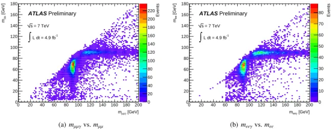
Figure 1: Distribution of the invariant massm_``γvs.m_``from photon candidates in the full 2011 data set after event selection, forµµγ(a) andeeγ(b) events.

Radiative decays in both theZ→µµγand theZ→eeγdecay channels are analyzed separately. The consistency of the results in both channels allows their combination into a single measurement.

3.1.1 Event selection in Z→``γanalyses

Events in theZ →µµγchannel are selected by requiring two muons with p_T > 15 GeV and|η| < 2.4.

While the trigger for these events only requires a match between a track in the ATLAS ID and the Muon Spectrometer (MS), the offline analysis selection also requires each muon to have at least one hit in the ATLAS Pixel detector, and six hits in the ATLAS Silicon Tracker. An isolation criterion is imposed, requiring that the ratio between the sum of thep_Tof the track withp_T>500 MeV in a cone of∆R=0.2 around each muon candidate, and the muon p_T, is less than 0.1.

Events in theZ → eeγ channel are selected by requiring two electrons with p_T > 15 GeV and

|η| < 1.37 or 1.52 ≤ |η| < 2.47, passing tight tracking and shower-shape criteria as described in detail in Ref. [9]. An E_T -based calorimetric isolation cut of 5 GeV, similar to that used for photons, is also applied to each electron.

The cross section forZ+jets events is about three orders of magnitude higher than forZ+γevents.

A non-negligible fraction of jets contain high-momentumπ⁰s decaying to collimated photon pairs which can fake photons and constitute a significant background in initial-state-radiation (ISR) photon samples.

In order to minimize the impact of such jet background in the radiativeZ samples, the three-body invariant massm_``γis restricted to be close tomZ. Figure 1 shows the two-dimensional distribution of the three-body``γinvariant mass vs. the two-body``invariant mass in data events passing the basic event- selection criteria listed above, separately for the electron and muon channels. The radiative Z events have a three-body invariant mass nearmZ, whereasZ+jets and ISR events lie in a distinct region of the phase-space. Thus, the three-body invariant mass is required to lie within 80 GeV<m_``γ<96 GeV and the di-lepton invariant mass is required to satisfy 40 GeV < m_`` < 83 GeV in both channels, minimiz- ing the contribution from Z+jets events while keeping that ofZ → ``γevents. If the radiated photon lies close (small∆Ri = p

(η^`ⁱ −η^γ)²+(φ^`ⁱ−φ^γ)²) to either of the leptons their electromagnetic showers can overlap, biasing the DV distributions towards lowerε_ID. A minimum∆Rrequirement between the photon and any lepton,∆R_min=min(∆R₁,∆R₂), is used to eliminate this effect.

In order to avoid a bias in ε_ID coming from the proximity of a lepton, a cut of ∆R_min > 0.2 is required on the photon in the muon channel, while a similar cut of ∆R_min > 0.4 is applied on the electron channel. The ε_ID obtained from these selections from MC simulated samples is compatible

(7)

60 70 80 90 100 110 120 130 140 1

10 102

103

(GeV)

γ

mee

60 70 80 90 100 110 120 130 140

Events / 1.6 GeV

1 10 102

103

Unconverted photon data fit signal background

ATLAS Preliminary = 7 TeV

s

Ldt = 4.9 fb-1

∫

60 70 80 90 100 110 120 130 140

1 10 102

103

(GeV)

γ µ

mµ

60 70 80 90 100 110 120 130 140

Events /1.6 GeV

1 10 102

103

Unconverted photon data fit signal background

s

Ldt = 4.91 fb-1

∫

60 70 80 90 100 110 120 130 140

1 10 102

103

(GeV)

γ

mee

60 70 80 90 100 110 120 130 140

Events / 1.6 GeV

1 10 102

103

Converted photon data fit signal background

s

Ldt = 4.91 fb-1

∫

60 70 80 90 100 110 120 130 140

1 10 102

103

(GeV)

γ µ

mµ

60 70 80 90 100 110 120 130 140

Events / 1.6 GeV

1 10 102

103

Converted photon data fit signal background

s

Ldt = 4.91 fb-1

∫

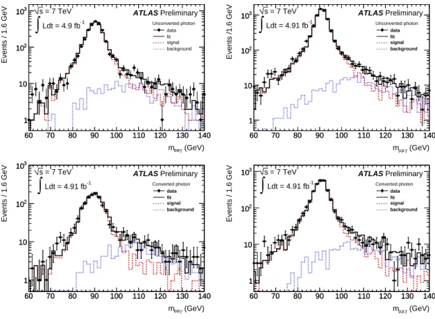
Figure 2: Invariant mass (m``γ) distribution of events selected in data after applying all theZ → ``γ selection criteria except that on m_``γ (left: ` = e; right: ` = µ), for unconverted (top) and converted (bottom) photon candidates. The result of the fit to the data distributions with the sum of the signal and background invariant mass distributions, as obtained from MC simulation, is superimposed.

within statistical uncertainty to that obtained from direct photons. The similarity is aided by the presence of the photon isolation requirement, which strongly suppresses fragmentation-type photons in the direct photon sample.

After the selection criteria is applied, 5995 events containing unconverted photons and 2705 containing converted photons are selected in the muon channel. In the electron channel, 2481 events containing unconverted photons and 1057 containing converted photons are selected.

3.1.2 Systematic uncertainties and impact of background in Z→``γanalyses

While the dominant uncertainty for these measurements is statistical, there is a small contribution from the presence of background in the selected photon sample, mostly fromZ+jets events. Them_``γinvari- ant mass shape is used as a discriminating variable to estimate the impact of this residual background contamination. The sum of them_``γsignal and background templates, obtained from MC simulation, is fitted to them_``γ distribution in the data by floating the relative normalization. The fits are performed by relaxing them_``γrequirement to 60 GeV< m_``γ <140 GeV. Figure 2 shows that the fitted sum is in good agreement with the data distribution. From the fit the signal purity is estimated to be (98.4±0.2)%

for the µµγ channel for unconverted photons, and (98.2±0.3)% for converted photons; for eeγ it is (98.0±0.2)% for unconverted photons and (96.0±0.3)% for converted photons. Both the signal and background templates are obtained from MC.

(8)

The measured change in the identification efficiency after applying the background subtraction is at most 0.7% for unconverted photons and 1.6% for converted photons in theZ → µµγchannel. For Z →eeγ, the difference is 0.8% for unconverted photons and 2.5% for converted photons. The number of events available in either the data sample or the MC sample does not allow this study to be carried out independently for each photon E_T andη region considered. Therefore, this overall uncertainty is assumed for each bin.

The proximity of the lepton to the radiated photon in either channel can potentially bias the measured ε_IDvalues. The∆Rcut is varied in the muon channel to 0.3 and 0.4, and the variation of the efficiency due to the variation of this cut is found to be negligible. Since in the electron channel the∆Rcut is large in comparison to the photon or electron cluster size, the impact of this systematic is also negligible.

The largest uncertainty in this analysis is statistical, and is found to be up to±5% in the high photon E_T(30−40 GeV) and highηregion.

3.2 Extrapolation from electrons fromZ→ e⁺e⁻decays

The underlying similarity between the electromagnetic showers induced by electrons and photons in the EMC can be exploited to extrapolate the εIDvalues from a pure sample of electrons in data, obtained from a tag-and-probe analysis of theZ → e⁺e⁻decays. The method provides a sample of photon-like showers with large statistics in the 20-80 GeV photonE_Trange.

The differences between photon and electron DVs is studied using MC simulation of direct photons and of electrons from the Z decay, separately for converted and unconverted photons. Converted photons typically reach the calorimeter as two overlapping showers and produce a shower similar to that of a single electron. For converted photons, the largest differences in shape to electrons are found in theR_φ distribution, which is sensitive to the electron and positron bending in ther−φplane. The converted photon cut onR_φis on the other hand relatively loose, reducing the impact of this difference. A test on MC simulated samples shows that, by directly applying the converted photon identification criteria to an electron sample, a difference of up to±3% between theε_IDobtained from these electrons and that expected for converted photons is found.

The showers induced by unconverted photons are more likely to initiate later than those induced by electrons, and thus tend to be narrower in the first layer of the EMC. Additionally, the lack of bending in theφ plane makes theR_φ distribution particularly different from that of electrons. Therefore, if the unconverted photon selection criteria are directly applied to an electron sample, a difference of the order of 20-30% between theε_IDobtained from these electrons and that expected for unconverted photons is found.

In order to use the information on DVs provided by electrons in data for the unconverted photon case, a transformation is used to map electrons to unconverted photons, which is invariant under those sources of systematic uncertainty present in the simulation which affect electrons and photons in the same way.

This transformation, hereby termed “Smirnov transform” from the Smirnov inverse probability integral transform [14], is applied to the DV computed from showers induced by electrons from data to reproduce a set of unconverted photons DVs as accurately and as independently as possible from the MC simulation.

If a given DV x is distributed according to the probability distribution function f(x) for electrons, and according tog(x) for photons, the respective cumulative distribution functions are:

F(x) = Z x

−∞

f(t)dt (2)

G(x) = Z x

−∞

g(t)dt (3)

(9)

Rφ

0.4 0.5 0.6 0.7 0.8 0.9 1

pdf

10-4

10-3

10-2

10-1 ≤ 30 GeV and 0.1 < |^η^|^≤^0.6 25 GeV < ET

electrons photons

ATLAS Preliminary Simulation

Rφ

0.4 0.5 0.6 0.7 0.8 0.9 1

CDF

0 0.2 0.4 0.6 0.8 1

electrons photons

electrons

0.4 0.5 0.6 0.7 0.8 0.9 1

photons

0.4 0.5 0.6 0.7 0.8 0.9 1

Smirnov Transform

Rφ

0.4 0.5 0.6 0.7 0.8 0.9 1

pdf

10-4

10-3

10-2

10-1 Transformed electrons

photons

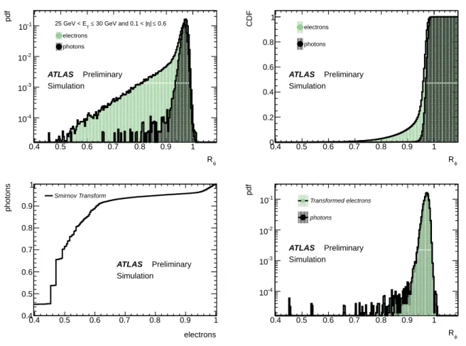
Figure 3:R_φprobability distribution function for unconverted photons and electrons (PDF, top left), and the respective cumulative distribution functions (CDF, top right). The bottom left plot shows the Smirnov transform function obtained by matching the cumulative distribution functions, whereas the bottom right plot shows the electronR_φprobability distribution functions after applying the Smirnov transformation, compared to that of photons.

The Smirnov transform function maps the electron DV x_e to a transformed variable x_γ, that is by construction distributed according tog(x), is then defined as:

x_γ =G⁻¹(F(xe)) (4)

Figure 3 shows an example of this procedure for theR_φvariables. Smirnov transform functions are separately computed for all nine DVs used in the tight selection criteria from MC simulated electrons and photons. Since the DVs for a given electron are transformed together, their initial correlations are preserved. The transformation functions are calculated separately for each photonE_Tandηbin, in order to minimize the impact of differences inE_Tandηdistributions between electrons and photons.

3.2.1 Event selection in electron extrapolation analysis

Following a tag-and-probe prescription [9], events are selected from data by requiring one electron (the tagelectron), to pass track–cluster matching, tight isolation, tracking and electron shower shape criteria.

The same isolation and tracking criteria are imposed on the second electron (theprobeelectron), but no shower-shape criteria. Since additional invariant-mass and jet-veto criteria are required at the event level

(10)

electron Fside

0.2 0.4 0.6 0.8 1

sidephoton F

0 0.1 0.2 0.3 0.4 0.5 0.6 0.7 0.8 0.9 1

≤ 0.8 η| 25 GeV and 0.6 < |

T≤ 20 GeV < E

Nominal geometry Distorted geometry

Figure 4: Smirnov transform as estimated using the nominal geometry for electrons and photons vs that obtained using a distorted geometry for the variableF_side(see Table 1) in the 20 GeV <E_T< 25 GeV region.

this selection results in a pure sample of probe electrons unbiased in the DVs. The detailed list of all cuts used to select theZ→e⁺e⁻sample is as follows:

• The two electron candidates are required to have opposite charge and 80 GeV<m_ee<100 GeV.

• Both electron candidates are required to passE_T >25 GeV and|η|<2.37, excluding the calorimeter transition region 1.37≤ |η|<1.52.

• Both electrons must pass tracking criteria from the tight electron selection. The number of silicon tracker hits must be at least seven while there must be a least one pixel hit. The tag electron is required to pass tight shower shape cuts.

• Both electrons must be isolated (E^iso_T (R=0.4)<5 GeV).

• No jet withE_T>20 GeV must be within a∆R<0.4 of the tag electron.

Close to 1.8 million tag or probe electron candidates are selected using 4.9 fb⁻¹ of 2011 data. The isolation prescription E^iso_T (R = 0.4) < 5 GeV has the added advantage of significantly improving the purity of the electron sample, which is important to reduce the systematic uncertainties from the Smirnov transformation procedure.

3.2.2 Systematic uncertainties and impact of background in electron extrapolation analysis Several sources of systematic uncertainty are considered for this analysis, and generally found to be larger for unconverted photons because of the tighter identification criteria and the larger differences with respect to electrons.

• The transformed electron sample ε_ID values are compared to the photon ones. The differences are found to be at most±2% for unconverted photons and at most±1% for converted photons.

They arise from differences in how photon and electron DVs are correlated, as well as differences in the η and p_T distributions within a given bin. These differences are added to the systematic uncertainties in the measuredε_IDvalues.

(11)

[GeV]

mee

60 80 100 120 140 160 180 200

Events/ 3.2 GeV

10-2

10-1

1 10 102

103

104

= 7 TeV s

L dt = 4.9 fb-1

∫

|η| < 0.6

ATLAS Preliminary

[GeV]

mee

60 80 100 120 140 160 180 200

Events/ 3.2 GeV

10-2

10-1

1 10 102

103

104

= 7 TeV s

L dt = 4.9 fb-1

∫

0.6 ≤ |η| < 1.37 ATLAS Preliminary

35 GeV probe≤ data 30 GeV < ET Background estimate

[GeV]

mee

60 80 100 120 140 160 180 200

Events/ 3.2 GeV

10-2

10-1

1 10 102

103

104

= 7 TeV s

L dt = 4.9 fb-1

∫

[GeV]

mee

60 80 100 120 140 160 180 200

Events/ 3.2 GeV

10-2

10-1

1 10 102

103

104

= 7 TeV s

L dt = 4.9 fb-1

∫

Figure 5: Two-electron candidate invariant mass distribution before applying tight shower shape cuts on the probe. The green shaded region shows the background template obtained from data by reversing the loose electron cuts, scaled to the high invariant mass region (mee>140 GeV). The points missing in the tail of the data distribution correspond to regions where there are no events in the data sample.

• The Smirnov transform functions are calculated alternatively using a MC simulation with additional passive material upstream of the calorimeters [9], to evaluate the sensitivity of the measured ε_ID values. The resulting uncertainties on theε_ID are found to be at most of±5% for converted photons and at most±15% for unconverted photons.

• The isolation criteria on the tag-and-probe electron sample is varied, to test the sensitivity to the presence of a residual background contamination. The resulting systematic uncertainty on theεID

is found to be always within±1%.

The largest source of systematic uncertainty arises from the sensitivity of the Smirnov transform function to the amount of material in front of the EMC. Figure 4 shows the Smirnov transform as obtained from electron and photon samples using the nominal geometry vs that using a geometry with additional dead material in front of the EMC. The Smirnov transforms are shown for the variableF_side(see Table 1) in the 20<E_T <25 GeV and|η|<0.6 region for unconverted photons.

The presence of anE_T-dependent background in the electron sample can bias theε_IDmeasurement.

This effect comes from the DV shapes of background electron candidates (charged hadrons mimicking electrons fromZdecays) being different from those of electrons for which the Smirnov transform functions are calculated. A data-driven estimate of the amount of background present in eachE_Tandηregion before and after the tight selection is performed. A background template is adjusted to the high end tail of the data distribution (mee> 140 GeV) in eachηandE_Tregion. The background template is obtained from those events where the probe fails to pass the loose electron cuts, as well as demanding that the probe is not isolated. Figure 5 shows themeedistribution along with the scaled background template for the 35< E_T <40 GeV region. The template correctly describes the high-end tail of themeedistribution

(12)

in allηandE_Tbins, both for the samples before and after the tight photon selections are applied on the Smirnov-transformed electrons. The fraction of background events estimated in this way is subtracted from the numerator and denominator in theε_IDcalculation, and the resulting values are compared to the nominal ones. Since the fractional amount of background is at the 1% level, the impact on the final efficiency figures is well below 1% and therefore negligible with respect to the other systematic uncertainties in this measurement.

3.3 Matrix Method

An inclusive sample of photon candidates is selected using single photon triggers by requiring at least one photon candidate with transverse energy E_T > 20 GeV. Only the photon candidates that pass a requirement on the calorimeter isolation, E^iso_T |_cut = 5 GeV are retained. In the collected sample, the observed numbers of photon candidates that pass (N_pass^T ) or fail (N_fail^T ) the tight photon identification criteria can be expressed in terms of signal (S) and background (B) candidates that pass or fail those requirements, leading to two equations with four unknowns:

N_pass^T = N_pass^S +N_pass^B

N_fail^T = N_fail^S +N_fail^B (5)

Using track isolation as a discriminating variable, two additional constraints can be placed on the four N_pass^S,B andN_fail^S,B yields. Track isolation is defined as the number of tracks in a cone of 0.001< ∆R <0.3 around the direction of a photon candidate, where a photon is considered track-isolated in the inner detector if no track with p_T > 500 MeV is found in the cone. Using the observed number of isolated photon candidates that either pass (N_pass^{T I} ) or fail (N_fail^{T I}) the tight identification criteria, the following expression is obtained:

N_pass^{T I} = ε^S_pN_pass^S +ε^B_pN_pass^B

N_fail^{T I} = ε^S_fN_fail^S +ε^B_fN_fail^B (6) If the track isolation efficiencies for signal and background candidates passing or failing the identification criteria (ε^S_p,ε^S_f,ε^B_p andε^B_f) are known, then the previous system of four equations can be solved to extract the four unknowns and thereforeε_ID= _NS^N^pass^S

pass+N^S

fail

. This is equivalent to determining the signal purity before (F) and after (P) the tight cuts, since:

F = εf −ε^b_f

ε^s_f −ε^b_f , (7)

P= εp−ε^b_p

ε^s_p−ε^b_p , (8)

whereεp ≡ ^N

passI so

N^T_pass is the fraction of tight photon candidates that pass the track isolation criteria. Measuring the tight level ε_ID values by obtaining the signal component before and after tight cuts in this way is referred to as the matrix method. The matrix method has the substantial advantage of providing a data- driven measurement ofε_IDover the whole photonE_Tspectrum of the photon candidate data sample.

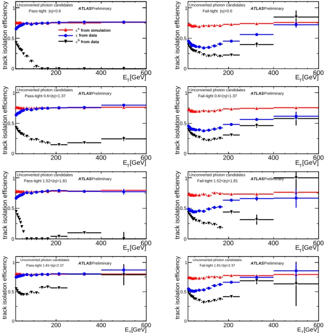
3.3.1 Determination of background track isolation efficiency and related systematic uncertainties The fake photon track isolation efficiencies (ε^Bp andε^B_f) are estimated from a data sample enriched in fake photons, selected by reversing the tight selections on the variables built using the highly segmented

(13)

[GeV]

ET

200 400 600

track isolation efficiency 0 0.5 1

from simulation εs

from data ε

from data εb Unconverted photon candidates

|<0.6 η

Pass-tight | ATLASPreliminary

[GeV]

ET

200 400 600

track isolation efficiency 0 0.5

1Unconverted photon candidates

|<0.6 η

Fail-tight | ATLASPreliminary

[GeV]

ET

200 400 600

|<1.37 η

Pass-tight 0.6<| ATLASPreliminary

[GeV]

ET

200 400 600

|<1.37 η

Fail-tight 0.6<| ATLASPreliminary

[GeV]

ET

200 400 600

track isolation efficiency ₀

0.5

|<1.81 η

[GeV]

ET

200 400 600

track isolation efficiency ₀

0.5

|<1.81 η

[GeV]

ET

200 400 600

track isolation efficiency

0 0.5

1 Unconverted photon candidates

|<2.37 η

[GeV]

ET

200 400 600

0 0.5

1 Unconverted photon candidates

|<2.37 η

Figure 6: Track isolation efficiencies for unconverted signal and background photon candidates passing (εp: left column) or failing (εf: right column) the relaxed-tight criteria, as measured in data and from MC simulated samples. The red triangular markers show the signal track isolation efficiency as obtained from simulation, whereas the black triangular markers show that of background, as determined from data. The blue circular markers show the overall track isolation efficiency found in data (signal and background together).

(14)

[GeV]

ET

200 400 600

track isolation efficiency 0 0.5 1

from simulation εs

from data ε

from data εb Converted photon candidates

|<0.6 η

Pass-tight | ATLAS Preliminary

[GeV]

ET

200 400 600

1 Converted photon candidates

|<0.6 η

Fail-tight | ATLASPreliminary

[GeV]

ET

200 400 600

|<1.37 η

[GeV]

ET

200 400 600

|<1.37 η

[GeV]

ET

200 400 600

|<1.81 η

[GeV]

ET

200 400 600

|<1.81 η

[GeV]

ET

200 400 600

0 0.5

|<2.37 η

[GeV]

ET

200 400 600

0 0.5

|<2.37 η

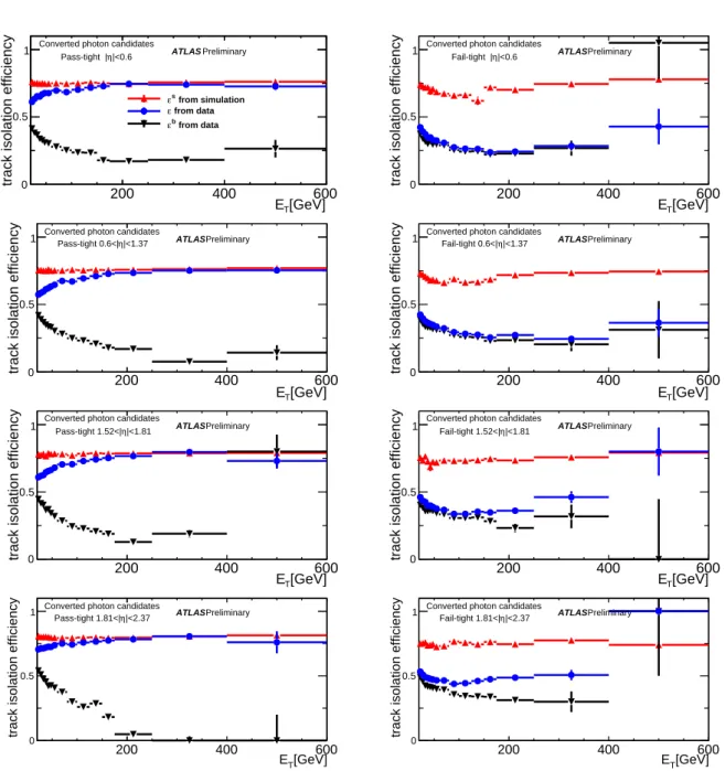
Figure 7: Track isolation efficiencies for converted signal and background photon candidates passing (εp: left column) or failing (εf: right column) the relaxed-tight criteria, as measured in data and from MC simulated samples. The red triangular markers show the signal track isolation efficiency as obtained from simulation, whereas the black triangular markers show that of background, as determined from data. The blue circular markers show the overall track isolation efficiency found in data (signal and background together).

(15)

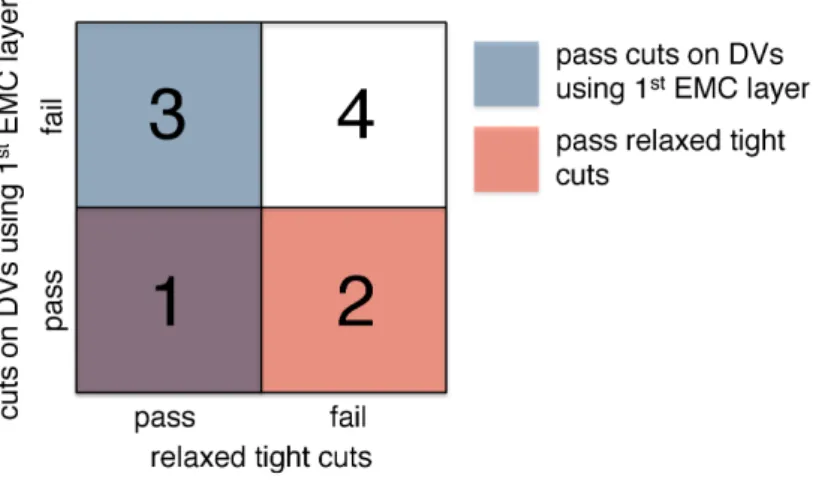
Figure 8: A graphical illustration of photon candidate classification in the data sample. Region 1: pass tight cuts; region 2: pass cuts on DVs using first EMC layer, but fail relaxed-tight cuts; region 3: pass relaxed-tight but fail cuts on DVs using first EMC layer; region 4: fail relaxed-tight and fail cuts on DVs using first EMC layer. Candidates in regions 3 and region 4 are used to estimate the track isolation efficiencies for backgroundε^b_pandε^b_f after subtraction of residual signal photons.

cells in the first layer of the EMCF_side,ws3,∆E, andE_ratio, which are only weakly correlated with track isolation. This sample contains no background passing tight identification cuts by construction, meaning that in order to obtainε^B_pa relaxed version of the tight cuts is defined. Therelaxedtight selection consists of those events which fail the cuts using DVs based on the first EMC layer, but which nevertheless pass the rest of the selection in the tight identification definition. Due to the very small correlation between the track isolation and the DVs based on the first EMC layer, the fake photon track isolation efficiency is similar for photon passing tight cuts or relaxed-tight criteria. This hypothesis is tested with di-jet MC simulated samples; the differences are included in the systematic uncertainties. Figure 6 and 7 show the behavior of the fake photon track isolation efficienciesε^B_p andε^B_f as a function of the photon candidate E_T in the four differentη regions for unconverted and converted photon candidates respectively. The purity and efficiency of the tight photon identification selection can be deduced from the values of these curves.

One of the major sources of systematic uncertainty comes from estimating the signal leakage into the background-enriched sample. Figure 8 shows the four regions created by the cut-reversal procedure.

Regions 3 and 4 are used to obtain the track isolation efficiency for background for those events passing and failing tight cuts, respectively. In order to obtain and subtract the signal leakage, (i.e. the fraction of the sample corresponding to signal events) in each of these regions, the signal efficiency for passing the respective criteria must be estimated. These fractions are obtained from MC simulation and are used to estimate and subtract the signal component from the background track isolation efficiency. Algebraically this is non-trivial, since it involves solving a system of non-linear equations through an iterative procedure. The possible systematic uncertainty in this recipe is estimated by carrying out the same procedure in a simulated sample and comparing the obtained background track isolation efficiencies with the true ones in the simulation. Unfortunately, a large component of the uncertainty arises from lack of events in the simulated sample used to cross-check the signal leakage subtraction procedure described above.

Since the statistical uncertainty is not disentangled from actual systematic uncertainties arising from correlations between track isolation and the DVs using the first EMC layer, the entire difference in MC is conservatively taken as a systematic uncertainty. For converted photons, this results in a systematic uncertainty estimate of up to ±20% for the efficiency of background events passing the tight photon selections.

(16)

3.3.2 Determination of signal track isolation efficiency and related systematic uncertainties The signal photon track isolation efficiency is obtained from direct photon MC simulation. Figure 6 and 7 show the behavior of the signal photon track isolation efficienciesε^S_p andε^S_f as a function of the photon candidate E_T in the four differentη regions for unconverted and converted photon candidates respectively.

The uncertainty on the signal photon track isolation efficiency is estimated by using the signal efficiency derived from a pure sample of electrons fromZ →e⁺e⁻decays. The difference between the data electron track isolation and that predicted by the MC simulation for unconverted photons is taken as a systematic uncertainty. For converted photons, an additional uncertainty originates from the difference of the track isolation efficiency between 1-track and 2-track conversions. This uncertainty is conservatively estimated as the difference between the efficiencies between unconverted and converted photons, with respect to which it should be smaller. The uncertainties in the signal track isolation efficiency are found to be relatively small, of up to±5% for converted photons failing the tight criteria and of±1% or less in the rest of the cases.

4 Comparison of the ε

_ID

data–driven measurements

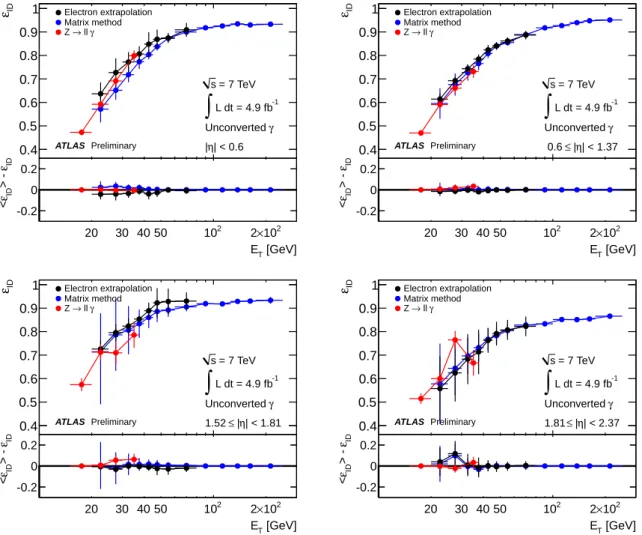
The ε_ID values obtained from the data-driven methods discussed in Section 3 are compared in Figs. 9 and 10 for unconverted and converted photons, respectively. The shaded bands in the figures represent the quadratic sum of the systematic and statistical uncertainties associated to each measurement. The results from the muon- and electron-radiativeZ analyses are shown as a single combined curve, while the matrix method and the electron extrapolation curves are shown separately.

In the overlapping photon E_T regions, the ε_IDvalues, which are independently measured from the different analyses, are compatible with each other up to the uncertainty assigned to each estimate, and no significant differences are observed. Relatively large fluctuations of the radiativeZdecay measurements are seen, due to their large statistical uncertainties.

Due to their good agreement and the independent data samples used, the different data-drivenεID

measurements can be combined in the overlapping photonE_Tregions. Since the three measurements use different data samples and independent MC simulations to estimateε_ID, their systematic and statistical uncertainties are largely uncorrelated.

The data-driven measurements show a similar dependence of the ε_ID with pileup. They are used to assign an uncertainty to the simulation of the detector response to pileup, as described in detail on Section 6.

Under the reasonable hypothesis of completely uncorrelated uncertainties, the weighted meanε_IDof the data-driven methods in every overlapping photonE_Tregion is computed as:

ε_ID±δε_ID= P

iwiε_IDi P

iwi

±





 X

i

w_i







−¹₂

w_i= 1

(δε_IDi)² (9)

where the sums run over the different data-driven results in a given (ET, η) bin, and the uncertainty on each measurementδεIDi is the quadrature sum of the associated statistical and systematic uncertainties.

For each averaged point theχ² = Pwi(ε_ID− ε_IDi)² is computed and compared to N−1, where N is the number of measurements combined for that point, andN−1 is the expectation value ofχ² from a Gaussian distribution. Only three bins among all photonη andE_T bins for unconverted and converted photons are found to have χ²/(N− 1) > 1. These χ² values are still smaller than 2, confirming the excellent compatibility between the different measurements. For the points with χ²/(N−1) > 1, the error on the combined valueδε_IDis increased by a factorS = p

χ²/(N−1), following the prescription in

(17)

102

IDε

0.4 0.5 0.6 0.7 0.8 0.9

1 Electron extrapolation Matrix method

γ

→ ll Z

= 7 TeV s

L dt = 4.9 fb-1

∫

γ

Unconverted

| < 0.6 η ATLAS Preliminary |

[GeV]

ET

20 30 40 50 10² 2×10²

IDε> - IDε<

-0.2 0

0.2 10²

IDε

0.4 0.5 0.6 0.7 0.8 0.9

γ

→ ll Z

= 7 TeV s

L dt = 4.9 fb-1

∫

γ

Unconverted

| < 1.37 η

≤ | 0.6 ATLAS Preliminary

[GeV]

ET

20 30 40 50 10² 2×10²

IDε> - IDε<

-0.2 0 0.2

102

IDε

0.4 0.5 0.6 0.7 0.8 0.9

γ

→ ll Z

= 7 TeV s

L dt = 4.9 fb-1

∫

γ

Unconverted

| < 1.81 η

[GeV]

ET

20 30 40 50 10² 2×10²

IDε> - IDε<

-0.2 0

0.2 10²

IDε

0.4 0.5 0.6 0.7 0.8 0.9

γ

→ ll Z

= 7 TeV s

L dt = 4.9 fb-1

∫

γ

Unconverted

| < 2.37 η

[GeV]

ET

20 30 40 50 10² 2×10²

IDε> - IDε<

-0.2 0 0.2

Figure 9: Comparison of the data-driven measurements of ε_ID for unconverted photons in the region 15 GeV < E_T < 300 GeV. The ε_ID curves are shown in four differentηregions. The results from the Z → µµγand Z → e⁺e⁻γ analyses are shown as a single curve. The uncertainty lines represent the quadratic sum of the statistical and systematic uncertainties estimated in each method. The difference of each of the curves to the weighted mean value is shown below.