EUROPEAN ORGANISATION FOR NUCLEAR RESEARCH (CERN)
CERN-PH-EP-2013-026
Submitted to: EPJC
Improved luminosity determination in p p pp p p collisions at √
sss = 7 TeV using the ATLAS detector at the LHC
The ATLAS Collaboration
Abstract
The luminosity calibration for the ATLAS detector at the LHC during ppcollisions at√
s=7 TeVin 2010 and 2011 is presented. Evaluation of the luminosity scale is performed using several luminosity- sensitive detectors, and comparisons are made of the long-term stability and accuracy of this calibra- tion applied to theppcollisions at√
s=7 TeV. A luminosity uncertainty ofδL/L =±3.5%is obtained for the47 pb−1 of data delivered to ATLAS in 2010, and an uncertainty ofδL/L =±1.8%is obtained for the5.5 fb−1 delivered in 2011.
arXiv:1302.4393v2 [hep-ex] 8 Jul 2013
Eur. Phys. J. C manuscript No.
(will be inserted by the editor)
Improved luminosity determination in p p pp p p collisions at √
sss = 7 TeV using the ATLAS detector at the LHC
The ATLAS Collaboration
1CERN, 1211 Geneve 23, Switzerland
Received: date / Accepted: date
Abstract The luminosity calibration for the ATLAS detec- tor at the LHC duringppcollisions at√
s=7 TeV in 2010 and 2011 is presented. Evaluation of the luminosity scale is performed using several luminosity-sensitive detectors, and comparisons are made of the long-term stability and accuracy of this calibration applied to the ppcollisions at
√s=7 TeV. A luminosity uncertainty ofδL/L =±3.5%
is obtained for the 47 pb−1of data delivered to ATLAS in 2010, and an uncertainty ofδL/L =±1.8% is obtained for the 5.5 fb−1delivered in 2011.
PACS 29.27.-a Charged-particle beams in accelerators· 13.75.Cs, 13.85.-t Proton-proton interactions
1 Introduction
An accurate measurement of the delivered luminosity is a key component of the ATLAS [1] physics programme. For cross-section measurements, the uncertainty on the deliv- ered luminosity is often one of the major systematic un- certainties. Searches for, and eventual discoveries of, new physical phenomena beyond the Standard Model also rely on accurate information about the delivered luminosity to evaluate background levels and determine sensitivity to the signatures of new phenomena.
This paper describes the measurement of the luminos- ity delivered to the ATLAS detector at the LHC in ppcol- lisions at a centre-of-mass energy of √
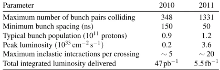
s=7 TeV during 2010 and 2011. The analysis is an evolution of the pro- cess documented in the initial ATLAS luminosity publica- tion [2] and includes an improved determination of the lumi- nosity in 2010 along with a new analysis for 2011. Table 1 highlights the operational conditions of the LHC during 2010 and 2011. The peak instantaneous luminosity deliv- ered by the LHC at the start of a fill increased fromLpeak=
Table 1 Selected LHC parameters forppcollisions at√
s=7 TeV in 2010 and 2011. Parameters shown are the best achieved for that year in normal physics operations.
Parameter 2010 2011
Maximum number of bunch pairs colliding 348 1331
Minimum bunch spacing (ns) 150 50
Typical bunch population (1011protons) 0.9 1.2 Peak luminosity(1033cm−2s−1) 0.2 3.6 Maximum inelastic interactions per crossing ∼5 ∼20 Total integrated luminosity delivered 47 pb−1 5.5 fb−1
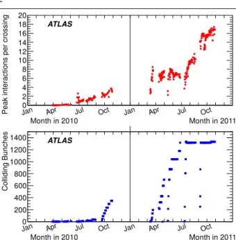
2.0×1032cm−2s−1in 2010 toLpeak=3.6×1033cm−2s−1 by the end of 2011. This increase results from both an in- creased instantaneous luminosity delivered per bunch cross- ing as well as a significant increase in the total number of bunches colliding. Figure 1 illustrates the evolution of these two parameters as a function of time. As a result of these changes in operating conditions, the details of the luminos- ity measurement have evolved from 2010 to 2011, although the overall methodology remains largely the same.
The strategy for measuring and calibrating the luminos- ity is outlined in Sect. 2, followed in Sect. 3 by a brief de- scription of the detectors used for luminosity determination.
Each of these detectors utilizes one or more luminosity al- gorithms as described in Sect. 4. The absolute calibration of these algorithms using beam-separation scans is described in Sect. 5, while a summary of the systematic uncertainties on the luminosity calibration as well as the calibration re- sults are presented in Sect. 6. Additional corrections which must be applied over the course of the 2011 data-taking pe- riod are described in Sect. 7, while additional uncertainties related to the extrapolation of the absolute luminosity cali- bration to the full 2010 and 2011 data samples are described in Sect. 8. The final results and uncertainties are summarized in Sect. 9.
Month in 2010 Month in 2011
Jan Apr Jul Oct Jan Apr Jul Oct
Peak interactions per crossing 0 2 4 6 8 10 12 14 16 18 20
ATLAS
Month in 2010 Month in 2011
Jan Apr Jul Oct Jan Apr Jul Oct
Colliding Bunches
0 200 400 600 800 1000 1200
1400 ATLAS
Fig. 1 Average number of inelasticppinteractions per bunch crossing at the start of each LHC fill (above) and number of colliding bunches per LHC fill (below) are shown as a function of time in 2010 and 2011.
The product of these two quantities is proportional to the peak lumi- nosity at the start of each fill.
2 Overview
The luminosityL of appcollider can be expressed as L =Rinel
σinel
(1) whereRinelis the rate of inelastic collisions andσinelis the pp inelastic cross-section. For a storage ring, operating at a revolution frequency frand withnbbunch pairs colliding per revolution, this expression can be rewritten as
L =µnbfr σinel
(2) whereµ is the average number of inelastic interactions per bunch crossing.
As discussed in Sects. 3 and 4, ATLAS monitors the delivered luminosity by measuring the observed interaction rate per crossing,µvis, independently with a variety of detec- tors and using several different algorithms. The luminosity can then be written as
L =µvisnbfr σvis
(3) whereσvis=ε σinelis the total inelastic cross-section mul- tiplied by the efficiencyεof a particular detector and algo- rithm, and similarlyµvis=ε µ. Sinceµvisis an experimen- tally observable quantity, the calibration of the luminosity scale for a particular detector and algorithm is equivalent to determining the visible cross-sectionσvis.
The majority of the algorithms used in the ATLAS lumi- nosity determination areevent countingalgorithms, where each particular bunch crossing is categorized as either pass- ing or not passing a given set of criteria designed to detect the presence of at least one inelasticppcollision. In the limit µvis1, the average number of visible inelastic interac- tions per bunch crossing is given by the simple expression µvis≈N/NBC whereN is the number of bunch crossings (or events) passing the selection criteria that are observed during a given time interval, and NBC is the total number of bunch crossings in that same interval. Asµvisincreases, the probability that two or moreppinteractions occur in the same bunch crossing is no longer negligible (a condition re- ferred to as “pile-up”), andµvisis no longer linearly related to the raw event count N. Instead µvis must be calculated taking into account Poisson statistics, and in some cases in- strumental or pile-up-related effects. In the limit where all bunch crossings in a given time interval contain an event, the event counting algorithm no longer provides any useful information about the interaction rate.
An alternative approach, which is linear to higher val- ues ofµvisbut requires control of additional systematic ef- fects, is that ofhit countingalgorithms. Rather than count- ing how many bunch crossings pass some minimum criteria for containing at least one inelastic interaction, in hit count- ing algorithms the number of detector readout channels with signals above some predefined threshold is counted. This provides more information per event, and also increases the µvisvalue at which the algorithm saturates compared to an event-counting algorithm. The extreme limit of hit count- ing algorithms, achievable only in detectors with very fine segmentation, are particle countingalgorithms, where the number of individual particles entering a given detector is counted directly. More details on how these different algo- rithms are defined, as well as the procedures for converting the observed event or hit rate into the visible interaction rate µvis, are discussed in Sect. 4.
As described more fully in Sect. 5, the calibration of σvis is performed using dedicated beam-separation scans, also known as van der Meer (vdM) scans, where the abso- lute luminosity can be inferred from direct measurements of the beam parameters [3, 4]. The delivered luminosity can be written in terms of the accelerator parameters as
L =nbfrn1n2
2π ΣxΣy (4)
where n1 and n2 are the bunch populations (protons per bunch) in beam 1 and beam 2 respectively (together form- ing the bunch population product), andΣx andΣy charac- terize the horizontal and vertical convolved beam widths. In avdMscan, the beams are separated by steps of a known distance, which allows a direct measurement ofΣxandΣy. Combining this scan with an external measurement of the
bunch population productn1n2provides a direct determina- tion of the luminosity when the beams are unseparated.
A fundamental ingredient of the ATLAS strategy to as- sess and control the systematic uncertainties affecting the absolute luminosity determination is to compare the mea- surements of several luminosity detectors, most of which use more than one algorithm to assess the luminosity. These multiple detectors and algorithms are characterized by sig- nificantly different acceptance, response to pile-up, and sen- sitivity to instrumental effects and to beam-induced back- grounds. In particular, since the calibration of the abso- lute luminosity scale is established in dedicatedvdMscans which are carried out relatively infrequently (in 2011 there was only one set of vdMscans at √
s=7 TeV for the en- tire year), this calibration must be assumed to be constant over long periods and under different machine conditions.
The level of consistency across the various methods, over the full range of single-bunch luminosities and beam condi- tions, and across many months of LHC operation, provides valuable cross-checks as well as an estimate of the detector- related systematic uncertainties. A full discussion of these is presented in Sects. 6–8.
The information needed for most physics analyses is an integrated luminosity for some well-defined data sam- ple. The basic time unit for storing luminosity information for physics use is the Luminosity Block (LB). The bound- aries of each LB are defined by the ATLAS Central Trigger Processor (CTP), and in general the duration of each LB is one minute. Trigger configuration changes, such as prescale changes, can only happen at luminosity block boundaries, and data are analysed under the assumption that each lumi- nosity block contains data taken under uniform conditions, including luminosity. The average luminosity for each de- tector and algorithm, along with a variety of general ATLAS data quality information, is stored for each LB in a relational database. To define a data sample for physics, quality crite- ria are applied to select LBs where conditions are accept- able, then the average luminosity in that LB is multiplied by the LB duration to provide the integrated luminosity de- livered in that LB. Additional corrections can be made for trigger deadtime and trigger prescale factors, which are also recorded on a per-LB basis. Adding up the integrated lumi- nosity delivered in a specific set of luminosity blocks pro- vides the integrated luminosity of the entire data sample.
3 Luminosity detectors
This section provides a description of the detector subsys- tems used for luminosity measurements. The ATLAS detec- tor is discussed in detail in Ref. [1]. The first set of detectors uses either event or hit counting algorithms to measure the luminosity on a bunch-by-bunch basis. The second set infers
the total luminosity (summed over all bunches) by monitor- ing detector currents sensitive to average particle rates over longer time scales. In each case, the detector descriptions are arranged in order of increasing magnitude of pseudora- pidity.1
The Inner Detector is used to measure the momentum of charged particles over a pseudorapidity interval of|η|<2.5.
It consists of three subsystems: a pixel detector, a silicon mi- crostrip tracker, and a transition-radiation straw-tube tracker.
These detectors are located inside a solenoidal magnet that provides a 2 T axial field. The tracking efficiency as a func- tion of transverse momentum (pT), averaged over all pseu- dorapidity, rises from 10% at 100 MeV to around 86% for pTabove a few GeV [5, 6]. The main application of the In- ner Detector for luminosity measurements is to detect the primary vertices produced in inelasticppinteractions.
To provide efficient triggers at low instantaneous lumi- nosity (L <1033 cm−2s−1), ATLAS has been equipped with segmented scintillator counters, the Minimum Bias Trigger Scintillators (MBTS). Located atz=±365 cm from the nominal interaction point (IP), and covering a rapidity range 2.09<|η|<3.84, the main purpose of the MBTS system is to provide a trigger on minimum collision activity during a pp bunch crossing. Light emitted by the scintil- lators is collected by wavelength-shifting optical fibers and guided to photomultiplier tubes. The MBTS signals, after being shaped and amplified, are fed into leading-edge dis- criminators and sent to the trigger system. The MBTS de- tectors are primarily used for luminosity measurements in early 2010, and are no longer used in the 2011 data.
The Beam Conditions Monitor (BCM) consists of four small diamond sensors, approximately 1 cm2 in cross- section each, arranged around the beampipe in a cross pat- tern on each side of the IP, at a distance ofz=±184 cm. The BCM is a fast device originally designed to monitor back- ground levels and issue beam-abort requests when beam losses start to risk damaging the Inner Detector. The fast readout of the BCM also provides a bunch-by-bunch lumi- nosity signal at|η|=4.2 with a time resolution of'0.7 ns.
The horizontal and vertical pairs of BCM detectors are read out separately, leading to two luminosity measurements la- belled BCMH and BCMV respectively. Because the accep- tances, thresholds, and data paths may all have small differ- ences between BCMH and BCMV, these two measurements are treated as being made by independent devices for cal- ibration and monitoring purposes, although the overall re- sponse of the two devices is expected to be very similar. In
1ATLAS uses a right-handed coordinate system with its origin at the nominal interaction point (IP) in the centre of the detector, and thez- axis along the beam line. Thex-axis points from the IP to the centre of the LHC ring, and they-axis points upwards. Cylindrical coordinates (r,φ)are used in the transverse plane, φ being the azimuthal angle around the beam line. The pseudorapidity is defined in terms of the polar angleθasη=−ln tan(θ/2).
the 2010 data, only the BCMH readout is available for lu- minosity measurements, while both BCMH and BCMV are available in 2011.
LUCID is a Cherenkov detector specifically designed for measuring the luminosity. Sixteen mechanically pol- ished aluminium tubes filled with C4F10 gas surround the beampipe on each side of the IP at a distance of 17 m, covering the pseudorapidity range 5.6 <|η| <6.0. The Cherenkov photons created by charged particles in the gas are reflected by the tube walls until they reach photomulti- plier tubes (PMTs) situated at the back end of the tubes. Ad- ditional Cherenkov photons are produced in the quartz win- dow separating the aluminium tubes from the PMTs. The Cherenkov light created in the gas typically produces 60–
70 photoelectrons per incident charged particle, while the quartz window adds another 40 photoelectrons to the signal.
If one of the LUCID PMTs produces a signal over a pre- set threshold (equivalent to'15 photoelectrons), a “hit” is recorded for that tube in that bunch crossing. The LUCID hit pattern is processed by a custom-built electronics card which contains Field Programmable Gate Arrays (FPGAs).
This card can be programmed with different luminosity al- gorithms, and provides separate luminosity measurements for each LHC bunch crossing.
Both BCM and LUCID are fast detectors with elec- tronics capable of making statistically precise luminosity measurements separately for each bunch crossing within the LHC fill pattern with no deadtime. These FPGA-based front-end electronics run autonomously from the main data acquisition system, and in particular are not affected by any deadtime imposed by the CTP.2
The Inner Detector vertex data and the MBTS data are components of the events read out through the data acquisi- tion system, and so must be corrected for deadtime imposed by the CTP in order to measure delivered luminosity. Nor- mally this deadtime is below 1%, but can occasionally be larger. Since not every inelastic collision event can be read out through the data acquisition system, the bunch crossings are sampled with a random or minimum bias trigger. While the triggered events uniformly sample every bunch cross- ing, the trigger bandwidth devoted to random or minimum bias triggers is not large enough to measure the luminosity separately for each bunch pair in a given LHC fill pattern during normal physics operations. For special running con- ditions such as thevdMscans, a custom trigger with partial event readout has been introduced in 2011 to record enough events to allow bunch-by-bunch luminosity measurements from the Inner Detector vertex data.
2The CTP inhibits triggers (causing deadtime) for a variety of reasons, but especially for several bunch crossings after a triggered event to al- low time for the detector readout to conclude. Any new triggers which occur during this time are ignored.
In addition to the detectors listed above, further luminosity-sensitive methods have been developed which use components of the ATLAS calorimeter system. These techniques do not identify particular events, but rather mea- sure average particle rates over longer time scales.
The Tile Calorimeter (TileCal) is the central hadronic calorimeter of ATLAS. It is a sampling calorimeter con- structed from iron plates (absorber) and plastic tile scintil- lators (active material) covering the pseudorapidity range
|η|<1.7. The detector consists of three cylinders, a cen- tral long barrel and two smaller extended barrels, one on each side of the long barrel. Each cylinder is divided into 64 slices in φ (modules) and segmented into three radial sampling layers. Cells are defined in each layer according to a projective geometry, and each cell is connected by op- tical fibers to two photomultiplier tubes. The current drawn by each PMT is monitored by an integrator system which is sensitive to currents from 0.1 nA to 1.2 mA with a time constant of 10 ms. The current drawn is proportional to the total number of particles interacting in a given TileCal cell, and provides a signal proportional to the total luminosity summed over all the colliding bunches present at a given time.
The Forward Calorimeter (FCal) is a sampling calorime- ter that covers the pseudorapidity range 3.2<|η|<4.9 and is housed in the two endcap cryostats along with the elec- tromagnetic endcap and the hadronic endcap calorimeters.
Each of the two FCal modules is divided into three lon- gitudinal absorber matrices, one made of copper (FCal-1) and the other two of tungsten (FCal-2/3). Each matrix con- tains tubes arranged parallel to the beam axis filled with liquid argon as the active medium. Each FCal-1 matrix is divided into 16φ-sectors, each of them fed by four inde- pendent high-voltage lines. The high voltage on each sector is regulated to provide a stable electric field across the liq- uid argon gaps and, similar to the TileCal PMT currents, the currents provided by the FCal-1 high-voltage system are di- rectly proportional to the average rate of particles interacting in a given FCal sector.
4 Luminosity algorithms
This section describes the algorithms used by the luminosity-sensitive detectors described in Sect. 3 to mea- sure the visible interaction rate per bunch crossing, µvis. Most of the algorithms used do not measure µvis directly, but rather measure some other rate which can be used to determineµvis.
ATLAS primarily uses event counting algorithms to measure luminosity, where a bunch crossing is said to con- tain an “event” if the criteria for a given algorithm to ob- serve one or more interactions are satisfied. The two main
algorithm types being used are EventOR (inclusive count- ing) and EventAND (coincidence counting). Additional al- gorithms have been developed using hit counting and aver- age particle rate counting, which provide a cross-check of the linearity of the event counting techniques.
4.1 Interaction rate determination
Most of the primary luminosity detectors consist of two symmetric detector elements placed in the forward (“A”) and backward (“C”) direction from the interaction point. For the LUCID, BCM, and MBTS detectors, each side is further segmented into a discrete number of readout segments, typ- ically arranged azimuthally around the beampipe, each with a separate readout channel. For event counting algorithms, a threshold is applied to the analoge signal output from each readout channel, and every channel with a response above this threshold is counted as containing a “hit”.
In an EventOR algorithm, a bunch crossing is counted if there is at least one hit on either the A side or the C side. As- suming that the number of interactions in a bunch crossing can be described by a Poisson distribution, the probability of observing an OR event can be computed as
PEvent_OR(µvisOR) =NOR
NBC =1−e−µvisOR. (5) Here the raw event countNORis the number of bunch cross- ings, during a given time interval, in which at least one pp interaction satisfies the event-selection criteria of the OR al- gorithm under consideration, andNBCis the total number of bunch crossings during the same interval. Solving forµvisin terms of the event counting rate yields:
µvisOR=−ln
1−NOR NBC
. (6)
In the case of an EventAND algorithm, a bunch cross- ing is counted if there is at least one hit on both sides of the detector. This coincidence condition can be satisfied either from a single ppinteraction or from individual hits on ei- ther side of the detector from differentppinteractions in the same bunch crossing. Assuming equal acceptance for sides A and C, the probability of recording an AND event can be expressed as
PEvent_AND(µvisAND) = NNAND
BC
=1−2e−(1+σvisOR/σvisAND)µvisAND/2 +e−(σvisOR/σvisAND)µvisAND.
(7)
This relationship cannot be inverted analytically to deter- mineµvisAND as a function ofNAND/NBC so a numerical in- version is performed instead.
Whenµvis1, event counting algorithms lose sensi- tivity as fewer and fewer events in a given time interval
have bunch crossings with zero observed interactions. In the limit whereN/NBC=1, it is no longer possible to use event counting to determine the interaction rateµvis, and more so- phisticated techniques must be used. One example is ahit countingalgorithm, where the number of hits in a given de- tector is counted rather than just the total number of events.
This provides more information about the interaction rate per event, and increases the luminosity at which the algo- rithm saturates.
Under the assumption that the number of hits in one pp interaction follows a Binomial distribution and that the num- ber of interactions per bunch crossing follows a Poisson dis- tribution, one can calculate the average probability to have a hit in one of the detector channels per bunch crossing as PHIT(µvisHIT) = NHIT
NBCNCH
=1−e−µvisHIT, (8) whereNHITandNBCare the total numbers of hits and bunch crossings during a time interval, andNCH is the number of detector channels. The expression above enablesµvisHITto be calculated from the number of hits as
µvisHIT=−ln(1−NNHIT
BCNCH). (9)
Hit counting is used to analyse the LUCID response (NCH=30) only in the high-luminosity data taken in 2011.
The lower acceptance of the BCM detector allows event counting to remain viable for all of 2011. The binomial as- sumption used to derive Eq. (9) is only true if the proba- bility to observe a hit in a single channel is independent of the number of hits observed in the other channels. A study of the LUCID hit distributions shows that this is not a cor- rect assumption, although the data presented in Sect. 8 also show that Eq. (9) provides a good description of howµvisHIT depends on the average number of hits.
An additional type of algorithm that can be used is a particle countingalgorithm, where some observable is di- rectly proportional to the number of particles interacting in the detector. These should be the most linear of all of the algorithm types, and in principle the interaction rate is di- rectly proportional to the particle rate. As discussed below, the TileCal and FCal current measurements are not exactly particle counting algorithms, as individual particles are not counted, but the measured currents should be directly pro- portional to luminosity. Similarly, the number of primary vertices is directly proportional to the luminosity, although the vertex reconstruction efficiency is significantly affected by pile-up as discussed below.
4.2 Online algorithms
The two main luminosity detectors used are LUCID and BCM. Each of these is equipped with customized FPGA-
based readout electronics which allow the luminosity algo- rithms to be applied “online” in real time. These electron- ics provide fast diagnostic signals to the LHC (within a few seconds), in addition to providing luminosity measurements for physics use. Each colliding bunch pair can be identified numerically by a Bunch-Crossing Identifier (BCID) which labels each of the 3564 possible 25 ns slots in one full rev- olution of the nominal LHC fill pattern. The online algo- rithms measure the delivered luminosity independently in each BCID.
For the LUCID detector, the two main algorithms are the inclusive LUCID_EventOR and the coincidence LUCID_EventAND. In each case, a hit is defined as a PMT signal above a predefined threshold which is set lower than the average single-particle response. There are two additional algorithms defined, LUCID_EventA and LUCID_EventC, which require at least one hit on ei- ther the A or C side respectively. Events passing these LUCID_EventA and LUCID_EventC algorithms are sub- sets of the events passing the LUCID_EventOR algorithm, and these single-sided algorithms are used primarily to monitor the stability of the LUCID detector. There is also a LUCID_HitOR hit counting algorithm which has been employed in the 2011 running to cross-check the linearity of the event counting algorithms at high values ofµvis.
For the BCM detector, there are two independent readout systems (BCMH and BCMV). A hit is defined as a single sensor with a response above the noise threshold. Inclusive OR and coincidence AND algorithms are defined for each of these independent readout systems, for a total of four BCM algorithms.
4.3 Offline algorithms
Additional offline analyses have been performed which rely on the MBTS and the vertexing capabilities of the Inner Detector. These offline algorithms use data triggered and read out through the standard ATLAS data acquisition sys- tem, and do not have the necessary rate capability to mea- sure luminosity independently for each BCID under normal physics conditions. Instead, these algorithms are typically used as cross-checks of the primary online algorithms under special running conditions, where the trigger rates for these algorithms can be increased.
The MBTS system is used for luminosity measurements only for the data collected in the 2010 run before 150 ns bunch train operation began. Events are triggered by the L1_MBTS_1 trigger which requires at least one hit in any of the 32 MBTS counters (which is equivalent to an inclu- sive MBTS_EventOR requirement). In addition to the trig- ger requirement, the MBTS_Timing analysis uses the time measurement of the MBTS detectors to select events where the time difference between the average hit times on the two
sides of the MBTS satisfies|∆t|<10 ns. This requirement is effective in rejecting beam-induced background events, as the particles produced in these events tend to traverse the de- tector longitudinally resulting in large values of|∆t|, while particles coming from the interaction point produce values of|∆t| '0. To form a∆t value requires at least one hit on both sides of the IP, and so the MBTS_Timing algorithm is in fact a coincidence algorithm.
Additional algorithms have been developed which are based on reconstructing interaction vertices formed by tracks measured in the Inner Detector. In 2010, the events were triggered by the L1_MBTS_1 trigger. The 2010 algo- rithm counts events with at least one reconstructed vertex, with at least two tracks withpT>100 MeV. This “primary vertex event counting” (PrimVtx) algorithm is fundamen- tally an inclusive event-counting algorithm, and the conver- sion from the observed event rate toµvisfollows Eq. (5).
The 2011 vertexing algorithm uses events from a trig- ger which randomly selects crossings from filled bunch pairs where collisions are possible. The average number of visible interactions per bunch crossing is determined by counting the number of reconstructed vertices found in each bunch crossing (Vertex). The vertex selection criteria in 2011 were changed to require five tracks with pT>400 MeV while also requiring tracks to have a hit in any active pixel detec- tor module along their path.
Vertex counting suffers from nonlinear behaviour with increasing interaction rates per bunch crossing, primarily due to two effects: vertex masking and fake vertices. Ver- tex masking occurs when the vertex reconstruction algo- rithm fails to resolve nearby vertices from separate inter- actions, decreasing the vertex reconstruction efficiency as the interaction rate increases. A data-driven correction is de- rived from the distribution of distances in the longitudinal direction (∆z) between pairs of reconstructed vertices. The measured distribution of longitudinal positions (z) is used to predict the expected∆zdistribution of pairs of vertices if no masking effect was present. Then, the difference be- tween the expected and observed∆zdistributions is related to the number of vertices lost due to masking. The procedure is checked with simulation for self-consistency at the sub- percent level, and the magnitude of the correction reaches up to+50% over the range of pile-up values in 2011 physics data. Fake vertices result from a vertex that would normally fail the requirement on the minimum number of tracks, but additional tracks from a second nearby interaction are er- roneously assigned so that the resulting reconstructed ver- tex satisfies the selection criteria. A correction is derived from simulation and reaches−10% in 2011. Since the 2010 PrimVtx algorithm requirements are already satisfied with one reconstructed vertex, vertex masking has no effect, al- though a correction must still be made for fake vertices.
4.4 Calorimeter-based algorithms
The TileCal and FCal luminosity determinations do not de- pend upon event counting, but rather upon measuring detec- tor currents that are proportional to the total particle flux in specific regions of the calorimeters. These particle counting algorithms are expected to be free from pile-up effects up to the highest interaction rates observed in late 2011(µ'20).
The Tile luminosity algorithm measures PMT currents for selected cells in a region near |η| ≈1.25 where the largest variations in current as a function of the luminosity are observed. In 2010, the response of a common set of cells was calibrated with respect to the luminosity measured by the LUCID_EventOR algorithm in a single ATLAS run. At the higher luminosities encountered in 2011, TileCal started to suffer from frequent trips of the low-voltage power sup- plies, causing the intermittent loss of current measurements from several modules. For these data, a second method is applied, based on the calibration of individual cells, which has the advantage of allowing different sets of cells to be used depending on their availability at a given time. The calibration is performed by comparing the luminosity mea- sured by the LUCID_EventOR algorithm to the individual cell currents at the peaks of the 2011 vdMscan, as more fully described in Sect. 7.5. While TileCal does not provide an independent absolute luminosity measurement, it enables systematic uncertainties associated with both long-term sta- bility andµ-dependence to be evaluated.
Similarly, the FCal high-voltage currents cannot be di- rectly calibrated during avdMscan because the total lumi- nosity delivered in these scans remains below the sensitivity of the current-measurement technique. Instead, calibrations were evaluated for each usable HV line independently by comparing to the LUCID_EventOR luminosity for a single ATLAS run in each of 2010 and 2011. As a result, the FCal also does not provide an independently calibrated luminos- ity measurement, but it can be used as a systematic check of the stability and linearity of other algorithms. For both the TileCal and FCal analyses, the luminosity is assumed to be linearly proportional to the observed currents after correct- ing for pedestals and non-collision backgrounds.
5 Luminosity calibration
In order to use the measured interaction rate µvis as a lu- minosity monitor, each detector and algorithm must be cali- brated by determining its visible cross-sectionσvis. The pri- mary calibration technique to determine the absolute lumi- nosity scale of each luminosity detector and algorithm em- ploys dedicatedvdMscans to infer the delivered luminosity at one point in time from the measurable parameters of the colliding bunches. By comparing the known luminosity de-
livered in thevdMscan to the visible interaction rate µvis, the visible cross-section can be determined from Eq. (3).
To achieve the desired accuracy on the absolute lumi- nosity, these scans are not performed during normal physics operations, but rather under carefully controlled conditions with a limited number of colliding bunches and a modest peak interaction rate(µ.2). At√
s=7 TeV three sets of such scans were performed in 2010 and one set in 2011.
This section describes thevdMscan procedure, while Sect. 6 discusses the systematic uncertainties on this procedure and summarizes the calibration results.
5.1 Absolute luminosity from beam parameters
In terms of colliding-beam parameters, the luminosityL is defined (for beams colliding with zero crossing angle) as L =nbfrn1n2
Z
ρˆ1(x,y)ρˆ2(x,y)dxdy (10) wherenbis the number of colliding bunch pairs, fris the ma- chine revolution frequency (11245.5 Hz for the LHC),n1n2 is the bunch population product, and ˆρ1(2)(x,y)is the nor- malized particle density in the transverse (x-y) plane of beam 1 (2) at the IP. Under the general assumption that the particle densities can be factorized into independent horizontal and vertical components, ( ˆρ(x,y) =ρx(x)ρy(y)), Eq. (10) can be rewritten as
L =nbfrn1n2Ωx(ρx1,ρx2)Ωy(ρy1,ρy2) (11) where
Ωx(ρx1,ρx2) = Z
ρx1(x)ρx2(x)dx
is the beam-overlap integral in thexdirection (with an anal- ogous definition in theydirection). In the method proposed by van der Meer [3] the overlap integral (for example in the xdirection) can be calculated as
Ωx(ρx1,ρx2) = Rx(0)
RRx(δ)dδ, (12)
whereRx(δ)is the luminosity (or equivalently µvis) — at this stage in arbitrary units — measured during a horizontal scan at the time the two beams are separated by the distance δ, andδ=0 represents the case of zero beam separation.
Defining the parameterΣxas Σx= 1
√ 2π
RRx(δ)dδ
Rx(0) , (13)
and similarly forΣy, the luminosity in Eq. (11) can be rewrit- ten as
L =nbfrn1n2
2π ΣxΣy, (14)
which enables the luminosity to be extracted from machine parameters by performing a vdM (beam-separation) scan.
In the case where the luminosity curveRx(δ)is Gaussian, Σx coincides with the standard deviation of that distribu- tion. Equation (14) is quite general;Σx andΣy, as defined in Eq. (13), depend only upon the area under the luminosity curve, and make no assumption as to the shape of that curve.
5.2vdMscan calibration
To calibrate a given luminosity algorithm, one can equate the absolute luminosity computed using Eq. (14) to the lu- minosity measured by a particular algorithm at the peak of the scan curve using Eq. (3) to get
σvis=µvisMAX2π ΣxΣy
n1n2
, (15)
whereµvisMAXis the visible interaction rate per bunch cross- ing observed at the peak of the scan curve as measured by that particular algorithm. Equation (15) provides a direct calibration of the visible cross-section σvis for each algo- rithm in terms of the peak visible interaction rate µvisMAX, the product of the convolved beam widths ΣxΣy, and the bunch population product n1n2. As discussed below, the bunch population product must be determined from an ex- ternal analysis of the LHC beam currents, but the remaining parameters are extracted directly from the analysis of the vdMscan data.
For scans performed with a crossing angle, where the beams no longer collide head-on, the formalism becomes considerably more involved [7], but the conclusions remain unaltered and Eqs. (13)–(15) remain valid. The non-zero vertical crossing angle used for some scans widens the lu- minosity curve by a factor that depends on the bunch length, the transverse beam size and the crossing angle, but reduces the peak luminosity by the same factor. The corresponding increase in the measured value ofΣyis exactly cancelled by the decrease inµvisMAX, so that no correction for the crossing angle is needed in the determination ofσvis.
One useful quantity that can be extracted from thevdM scan data for each luminosity method and that depends only on the transverse beam sizes, is the specific luminos- ityLspec:
Lspec=L/(nbn1n2) = fr
2π ΣxΣy. (16)
Comparing the specific luminosity values (i.e. the inverse product of the convolved beam sizes) measured in the same scan by different detectors and algorithms provides a direct check on the mutual consistency of the absolute luminosity scale provided by these methods.
5.3vdMscan data sets
The beam conditions during the dedicated vdMscans are different from the conditions in normal physics fills, with fewer bunches colliding, no bunch trains, and lower bunch intensities. These conditions are chosen to reduce various systematic uncertainties in the scan procedure.
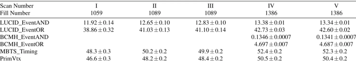
A total of five vdMscans were performed in 2010, on three different dates separated by weeks or months, and an additional twovdMscans at√
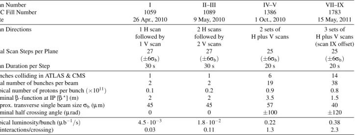
s=7 TeV were performed in 2011 on the same day to calibrate the absolute luminos- ity scale. As shown in Table 2, the scan parameters evolved from the early 2010 scans where single bunches and very low bunch charges were used. The final set of scans in 2010 and the scans in 2011 were more similar, as both used close- to-nominal bunch charges, more than one bunch colliding, and typical peakµvalues in the range 1.3–2.3.
Generally, eachvdMscan consists of two separate beam scans, one where the beams are separated by up to±6σbin thexdirection keeping the beams centred in y, and a sec- ond where the beams are separated in theydirection with the beams centred inx, whereσbis the transverse size of a single beam. The beams are moved in a certain number of scan steps, then data are recorded for 20–30 seconds at each step to obtain a statistically significant measurement in each luminosity detector under calibration. To help assess experimental systematic uncertainties in the calibration pro- cedure, two sets of identical vdMscans are usually taken in short succession to provide two independent calibrations under similar beam conditions. In 2011, a third scan was performed with the beams separated by 160µm in the non- scanning plane to constrain systematic uncertainties on the factorization assumption as discussed in Sect. 6.1.11.
Since the luminosity can be different for each colliding bunch pair, both because the beam sizes can vary bunch-to- bunch but also because the bunch population productn1n2
can vary at the level of 10–20%, the determination ofΣx/y and the measurement ofµvisMAXat the scan peak must be per- formed independently for each colliding BCID. As a result, the May 2011 scan provides 14 independent measurements of σvis within the same scan, and the October 2010 scan provides 6. The agreement among theσvisvalues extracted from these different BCIDs provides an additional consis- tency check for the calibration procedure.
5.4vdMscan analysis
For each algorithm being calibrated, thevdMscan data are analysed in a very similar manner. For each BCID, the spe- cific visible interaction rate µvis/(n1n2) is measured as a function of the “nominal” beam separation,i.e.the separa- tion specified by the LHC control system for each scan step.
The specific interaction rate is used so that the result is not
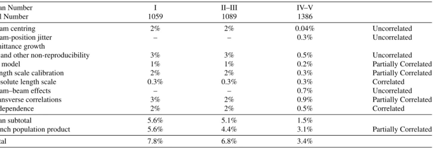
Table 2 Summary of the main characteristics of the 2010 and 2011vdMscans performed at the ATLAS interaction point. Scan directions are indicated by “H” for horizontal and “V” for vertical. The values of luminosity/bunch andµare given for zero beam separation.
Scan Number I II–III IV–V VII–IX
LHC Fill Number 1059 1089 1386 1783
Date 26 Apr., 2010 9 May, 2010 1 Oct., 2010 15 May, 2011
Scan Directions 1 H scan 2 H scans 2 sets of 3 sets of
followed by followed by H plus V scans H plus V scans
1 V scan 2 V scans (scan IX offset)
Total Scan Steps per Plane 27 27 25 25
(±6σb) (±6σb) (±6σb) (±6σb)
Scan Duration per Step 30 s 30 s 20 s 20 s
Bunches colliding in ATLAS & CMS 1 1 6 14
Total number of bunches per beam 2 2 19 38
Typical number of protons per bunch(×1011) 0.1 0.2 0.9 0.8
Nominalβ-function at IP [β?] (m) 2 2 3.5 1.5
Approx. transverse single beam sizeσb(µm) 45 45 57 40
Nominal half crossing angle (µrad) 0 0 ±100 ±120
Typical luminosity/bunch (µb−1/s) 4.5·10−3 1.8·10−2 0.22 0.38
µ(interactions/crossing) 0.03 0.11 1.3 2.3
Horizontal Beam Separation [mm]
]-2 p)11 (10-1 ) [BC2 n 1/(n visµ
0 0.05 0.1 0.15 0.2 0.25
ATLAS
Horizontal Beam Separation [mm]
-0.2 -0.1 0 0.1 0.2
dataσdata-fit
-3 -2 -1 0 1 2 3
Fig. 2 Specific visible interaction rate versus nominal beam separation for the BCMH_EventOR algorithm during scan VII in the horizontal plane for BCID 817. The residual deviation of the data from the Gaus- sian plus constant term fit, normalized at each point to the statistical uncertainty(σdata), is shown in the bottom panel.
affected by the change in beam currents over the duration of the scan. An example of thevdMscan data for a single BCID from scan VII in the horizontal plane is shown in Fig. 2.
The value ofµvisis determined from the raw event rate using the analytic function described in Sect. 4.1 for the in- clusive EventOR algorithms. The coincidence EventAND algorithms are more involved, and a numerical inversion is
performed to determineµvisfrom the raw EventAND rate.
Since the EventANDµdetermination depends onσvisANDas well asσvisOR, an iterative procedure must be employed. This procedure is found to converge after a few steps.
At each scan step, the beam separation and the visible interaction rate are corrected for beam–beam effects as de- scribed in Sect. 5.8. These corrected data for each BCID of each scan are then fitted independently to a characteris- tic function to provide a measurement of µvisMAX from the peak of the fitted function, while Σ is computed from the integral of the function, using Eq. (13). Depending upon the beam conditions, this function can be a double Gaus- sian plus a constant term, a single Gaussian plus a constant term, a spline function, or other variations. As described in Sect. 6, the differences between the different treatments are taken into account as a systematic uncertainty in the calibra- tion result.
One important difference in thevdMscan analysis be- tween 2010 and 2011 is the treatment of the backgrounds in the luminosity signals. Figure 3 shows the average BCMV_EventOR luminosity as a function of BCID dur- ing the May 2011 vdM scan. The 14 large spikes around L '3×1029cm−2s−1 are the BCIDs containing collid- ing bunches. Both the LUCID and BCM detectors observe some small activity in the BCIDs immediately following a collision which tends to die away to some baseline value with several different time constants. This “afterglow” is most likely caused by photons from nuclear de-excitation, which in turn is induced by the hadronic cascades initiated by ppcollision products. The level of the afterglow back- ground is observed to be proportional to the luminosity in the colliding BCIDs, and in thevdMscans this background can be estimated by looking at the luminosity signal in the BCID immediately preceding a colliding bunch pair. A sec-
Bunch Crossing Number 0 500 1000 1500 2000 2500 3000 3500 ]-1 s-2 cm27Avg. Luminosity [10
10-3
10-2
10-1
1 10 102
103
104
105
BCMV_EventOR ATLAS
Fig. 3 Average observed luminosity per BCID from BCMV_EventOR in the May 2011vdMscan. In addition to the 14 large spikes in the BCIDs where two bunches are colliding, induced “afterglow” activity can also be seen in the following BCIDs. Single-beam background sig- nals are also observed in BCIDs corresponding to unpaired bunches (24 in each beam).
ond background contribution comes from activity correlated with the passage of a single beam through the detector. This
“single-beam” background, seen in Fig. 3 as the numerous small spikes at the 1026cm−2s−1 level, is likely a combi- nation of beam-gas interactions and halo particles which intercept the luminosity detectors in time with the main beam. It is observed that this single-beam background is proportional to the bunch charge present in each bunch, and can be considerably different for beams 1 and 2, but is otherwise uniform for all bunches in a given beam. The single-beam background underlying a collision BCID can be estimated by measuring the single-beam backgrounds in unpaired bunches and correcting for the difference in bunch charge between the unpaired and colliding bunches. Adding the single-beam backgrounds measured for beams 1 and 2 then gives an estimate for the single-beam background present in a colliding BCID. Because the single-beam back- ground does not depend on the luminosity, this background can dominate the observed luminosity response when the beams are separated.
In 2010, these background sources were accounted for by assuming that any constant term fitted to the observed scan curve is the result of luminosity-independent back- ground sources, and has not been included as part of the luminosity integrated to extract Σx orΣy. In 2011, a more detailed background subtraction is first performed to cor- rect each BCID for afterglow and single-beam backgrounds, then any remaining constant term observed in the scan curve has been treated as a broad luminosity signal which con- tributes to the determination ofΣ.
The combination of onex scan and oney scan is the minimum needed to perform a measurement ofσvis. The av- erage value of µvisMAXbetween the two scan planes is used in the determination ofσvis, and the correlation matrix from each fit between µvisMAX andΣ is taken into account when evaluating the statistical uncertainty.
[mb]
σvis
LUCID_EventOR 42 42.2 42.4 42.6 42.8 43 43.2 43.4 43.6 43.8
BCID
81 131 181 231 281 331 817 867 917 967 2602 2652 2702 2752
Scan VII Scan VII Mean Scan VIII Scan VIII Mean Overall Weighted Mean
0.9% from
±
ATLAS
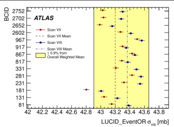
Fig. 4 Measuredσvisvalues for LUCID_EventOR by BCID for scans VII and VIII. The error bars represent statistical errors only. The verti- cal lines indicate the weighted average over BCIDs for scans VII and VIII separately. The shaded band indicates a±0.9% variation from the average, which is the systematic uncertainty evaluated from the per- BCID and per-scanσvisconsistency.
Each BCID should measure the sameσvisvalue, and the average over all BCIDs is taken as theσvismeasurement for that scan. Any variation inσvis between BCIDs, as well as between scans, reflects the reproducibility and stability of the calibration procedure during a single fill.
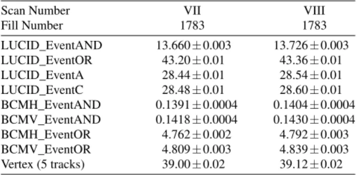
Figure 4 shows the σvis values determined for LUCID_EventOR separately by BCID and by scan in the May 2011 scans. The RMS variation seen between the σvisresults measured for different BCIDs is 0.4% for scan VII and 0.3% for scan VIII. The BCID-averagedσvis val- ues found in scans VII and VIII agree to 0.5% (or bet- ter) for all four LUCID algorithms. Similar data for the BCMV_EventOR algorithm are shown in Fig. 5. Again an RMS variation between BCIDs of up to 0.55% is seen, and a difference between the two scans of up to 0.67% is observed for the BCM_EventOR algorithms. The agree- ment in the BCM_EventAND algorithms is worse, with an RMS around 1%, although these measurements also have significantly larger statistical errors.
Similar features are observed in the October 2010 scan, where theσvisresults measured for different BCIDs, and the BCID-averaged σvis value found in scans IV and V agree to 0.3% for LUCID_EventOR and 0.2% for LUCID_EventAND. The BCMH_EventOR results agree between BCIDs and between the two scans at the 0.4%
level, while the BCMH_EventAND calibration results are consistent within the larger statistical errors present in this measurement.
[mb]
σvis
BCMV_EventOR 4.68 4.7 4.72 4.74 4.76 4.78 4.8 4.82 4.84 4.86 4.88
BCID
81 131 181 231 281 331 817 867 917 967 2602 2652 2702 2752
Scan VII Scan VII Mean Scan VIII Scan VIII Mean Overall Weighted Mean
0.9% from
±
ATLAS
Fig. 5 Measuredσvisvalues for BCMV_EventOR by BCID for scans VII and VIII. The error bars represent statistical errors only. The verti- cal lines indicate the weighted average over BCIDs for Scans VII and VIII separately. The shaded band indicates a±0.9% variation from the average, which is the systematic uncertainty evaluated from the per- BCID and per-scanσvisconsistency.
5.5 Internal scan consistency
The variation between the measuredσvis values by BCID and between scans quantifies the stability and reproducibil- ity of the calibration technique. Comparing Figs. 4 and 5 for the May 2011 scans, it is clear that some of the vari- ation seen in σvis is not statistical in nature, but rather is correlated by BCID. As discussed in Sect. 6, the RMS vari- ation ofσvisbetween BCIDs within a given scan is taken as a systematic uncertainty in the calibration technique, as is the reproducibility ofσvis between scans. The yellow band in these figures, which represents a range of±0.9%, shows the quadrature sum of these two systematic uncertainties.
Similar results are found in the final scans taken in 2010, although with only 6 colliding bunch pairs there are fewer independent measurements to compare.
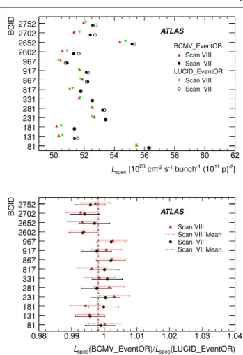
Further checks can be made by considering the distri- bution of Lspec defined in Eq. (16) for a given BCID as measured by different algorithms. Since this quantity de- pends only on the convolved beam sizes, consistent results should be measured by all methods for a given scan. Fig- ure 6 shows the measuredLspecvalues by BCID and scan for LUCID and BCMV algorithms, as well as the ratio of these values in the May 2011 scans. Bunch-to-bunch varia- tions of the specific luminosity are typically 5–10%, reflect- ing bunch-to-bunch differences in transverse emittance also seen during normal physics fills. For each BCID, however, all algorithms are statistically consistent. A small system- atic reduction inLspeccan be observed between scans VII and VIII, which is due to emittance growth in the colliding beams.
Figures 7 and 8 show theΣx andΣyvalues determined by the BCM algorithms during scans VII and VIII, and for
-2]
11 p)
-1 (10 bunch s-1
cm-2
[1028
Lspec
50 52 54 56 58 60 62
BCID
81 131 181 231 281 331 817 867 917 967 2602 2652 2702 2752
BCMV_EventOR Scan VIII Scan VII LUCID_EventOR
Scan VIII Scan VII ATLAS
(LUCID_EventOR) Lspec
(BCMV_EventOR)/
Lspec
0.98 0.99 1 1.01 1.02 1.03 1.04
BCID
81 131 181 231 281 331 817 867 917 967 2602 2652 2702 2752
Scan VIII Scan VIII Mean Scan VII Scan VII Mean ATLAS
Fig. 6 Specific luminosity determined by BCMV and LUCID per BCID for scans VII and VIII. The figure on the top shows the specific luminosity values determined by BCMV_EventOR and LUCID_EventOR, while the figure on the bottom shows the ratios of these values. The vertical lines indicate the weighted average over BCIDs for scans VII and VIII separately. The error bars represent sta- tistical uncertainties only.
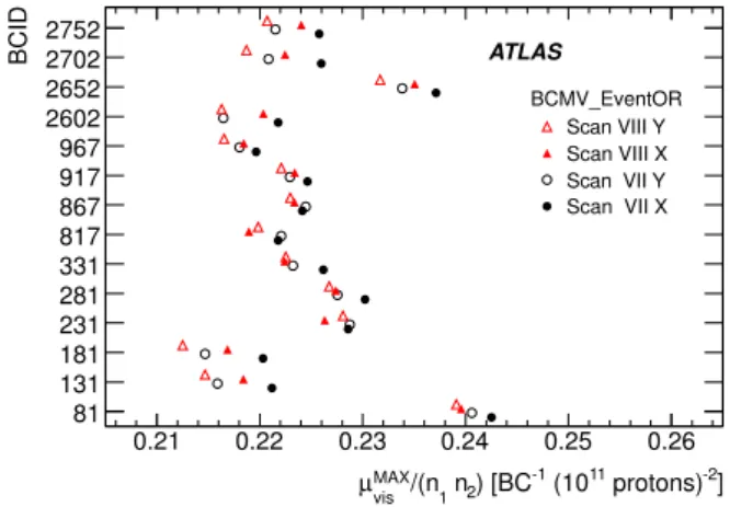
each BCID a clear increase can be seen with time. This emit- tance growth can also be seen clearly as a reduction in the peak specific interaction rateµvisMAX/(n1n2)shown in Fig. 9 for BCMV_EventOR. Here the peak rate is shown for each of the four individual horizontal and vertical scans, and a monotonic decrease in rate is generally observed as each in- dividual scan curve is recorded. The fact that theσvis val- ues are consistent between scan VII and scan VIII demon- strates that to first order the emittance growth cancels out of the measured luminosity calibration factors. The residual uncertainty associated with emittance growth is discussed in Sect. 6.
5.6 Bunch population determination
The dominant systematic uncertainty on the 2010 luminos- ity calibration, and a significant uncertainty on the 2011 cal- ibration, is associated with the determination of the bunch