Technical Implementation of Daily Adaptive Proton Therapy

(1)

Research Collection

Doctoral Thesis

Technical Implementation of Daily Adaptive Proton Therapy

Author(s):

Matter, Michael Publication Date:

2020

Permanent Link:

https://doi.org/10.3929/ethz-b-000460899

Rights / License:

In Copyright - Non-Commercial Use Permitted

This page was generated automatically upon download from the ETH Zurich Research Collection. For more information please consult the Terms of use.

ETH Library

(2)

DISS. ETH NO. 27104

Technical Implementation of Daily Adaptive Proton Therapy

A thesis submitted to attain the degree of DOCTOR OF SCIENCES of ETH ZURICH

(Dr. sc. ETH Zurich)

presented by Michael Matter

M. sc. ETH Zurich

born on 26.09.1991 citizen of Kölliken/AG

accepted on the recommendation of

Antony J Lomax Francesca Albertini

Jan-Jakob Sonke Andreas Vaterlaus

2020

(3)

ii

(4)

Acknowledgments

When I arrived at the Center for Proton Therapy at the Paul Scherrer Institute in summer of 2017, there were two PhD positions founded by a Swiss National Science Foundation project with the title "Towards Daily Adapted Proton Therapy at PSI." The proposal for this project was written by Francesca Albertini, which was my main supervisor for this project. Lena Nenoff and myself became the two PhD students, which together with Francesca, started to work towards solving the problems of DAPT. First and foremost I would like to thank Francesca. From the start, I could profit from her clear vision of DAPT and her huge clinical experience. Many of my achievements in these last years were only possible thanks to her supervision and our great working relationship. Secondly, I would like to thank Lena. It was great to have a colleague working side-by-side with the same final goal in mind. And thirdly, I would like to thank Tony Lomax, who was my supervising professor. Tony is the best motivational speaker I ever met, he helped and guided me through out the project.

And then obviously there were a lot of people in CPT, who helped me in hundreds of occasions. I want to say a huge thank you to Gabriel Meier, who supervised and supported me in software development tasks. His help, when I was close to despair because I could not find a software bug for multiple days, was priceless. Not only Gabriel, but the whole Medical Software team and Alex Mayor were very supportive, all the time.

For the occasions when we did measurements at the Gantry and nothing worked, which was usually the case, we called Serena, Benno, Michael, Oxana, Dorta, Pablo, Martina, Zema or anybody we could think of, and they were always trying their best to help us, also at weekends or at night. Also the medical doctors were very approachable at CPT and helped us a lot with discussing workflow and user interface issues. And finally, I would like to thank all other students and postdocs at CPT, who were responsible for an awesome working environment. The cake breaks, swimming over lunch and the supportive climate in our office, made my PhD experience truly enjoyable.

iii

(5)

iv

(6)

Abstract

Proton therapy is a specialized approach for highly conformal radiotherapy for cancer patients. Because of the favourable physical properties of accelerated protons compared to X-rays, in proton therapy less healthy tissue needs to be irradiated to get the same result in tumor control. The drawback of proton therapy however, is its sensitivity to density changes in the beam path for example due to positioning uncertainty or due to anatomical changes. The solution is adapting the delivered dose distribution to the most recent patient geometry and correcting for any changes. Daily Adaptive Proton Therapy (DAPT) is our approach for addressing this problem, which entails an online adaption of the treatment plan according to a CT image obtained just minutes before delivery start.

Although the clinical benefits of such adaption methods are obvious and online adaption in X-ray therapy becomes more and more available, proton specific challenges prevented a clinical introduction of DAPT so far.

During the last three years the problems preventing online adaption in proton therapy were identified and tackled one by one. The result is described in this thesis. The main technical problems encountered were the development of the online optimization algorithms, the workflow definition and the design of the quality assurance process. As the whole adaption process needs to be conducted while the patient lies on the treatment couch, we aimed at no more than 5-10 minutes between the end of the daily image acquisition and treatment start. Therefore, large efforts were spent in speeding up the calculational steps and streamlining the workflow, such that both, the therapy is com- fortable for the patient and can be conducted without increase in treatment facility occupancy. We developed a workflow and addressed all of its technical challenges to be able to treat the first patient with DAPT at Paul Scherrer Intitut (PSI). To gain the first clinical experience we chose a simple case, where no structure deformations are expected, but anatomical changes still occur. This approach severely limits the applicability of the method, but also greatly simplifies the problem and enables a timely introduction into the clinical routine. From the start, the method was developed in close collaboration with the treatment planning system development team and future users (e.g. medical physicists, MTRAs and medical doctors) with the goal to make a clinically usable and valuable product. Finally, a prototype software, which features all necessary algorithms for DAPT and has a user interface, which guides the user through the whole workflow was developed and tested.

The prototype was tested in an end-to-end test with an anthropomorphic phantom and we could show that the method is safe, the resulting dose distribution matches the predictions and that the whole workflow can be conducted without significant increase in treatment time compared to non-adaptive therapy. As a side product of the development for DAPT, a fast implementation for plan optimization was developed, which can also be used for non-adaptive therapy. This fast implementation, which is up to a hundred times faster than our current clinical implementation, will greatly increase the comfort

v

(7)

vi

for designing treatment plans. Further, in the course of the quality assurance investigation for DAPT, we found strong arguments favouring measurement free patient specific verification over conventional measurements. This will help the reduction of necessary measurements in the clinical practice also for non-adaptive therapy and will reduce the overall cost of proton therapy.

In this thesis, first proton therapy is introduced and then the literature concerning online adaption in proton therapy is reviewed in chapter2. The next four chapters are papers addressing the problems encountered in DAPT. The core of this work can be found in chapter3, where the solution we found for treating the first patient with DAPT at PSI is described. The other three chapters, in the form of published papers, address specific technical challenges in the DAPT workflow. Finally, the remaining problems, the advantages and the drawback of the chosen solution and future work is discussed in chapter7.

With the work described in this thesis, the foundation is laid for the first clinical delivery of an online adapted proton therapy plan. While many problems remain unsolved, the approach to gain the first clinical experience is outlined and after transforming the prototype into a clinical product, the commissioning of the new method can start. All necessary work before the first online adaptive patient treatment in proton therapy is outlined and the first treatment is scheduled for the first quarter of 2021.

(8)

Zusammenfassung

Protonentherapie ist ein spezialisierter Ansatz für die Behandlung von Krebs Patienten, welche eine besonders konforme Dosisverteilung ermöglicht. Wegen der vorteilhaften physikalischen Eigenschaften von beschleunigten Protonen, im Vergleich mit Photonen, wird in der Protonentherapie weniger gesundes Gewebe bestrahlt um die gleiche Tu- morkontrolle zu erreichen. Der Nachteil hingegen ist die Empfindlichkeit der Proto- nentherapie auf Änderungen der Dichte im Strahlverlauf zum Beispiel aufgrund von anatomischen Veränderungen. Dieses Problem kann durch tägliches Anpassen der Do- sisverteilung an die aktuellste Patienten Anatomie gelöst werden. Täglich adaptive Pro- tonentherapie (DAPT) ist unser Ansatz dieses Problem anzugehen, indem wir jeden Tag ein neues CT Bild aufnehmen und die Behandlung anhand diesem korrigieren. Obwohl der klinische Nutzen einer solchen adaptiven Behandlung offensichtlich ist und derartige online Korrekturen bei der Behandlung mit Röntgenstrahlen bereits eingesetzt werden, verursachen die Protonen spezifische Probleme welche, die klinischen Einführung bisher verhinderten.

In den letzten drei Jahren wurden die Probleme systematisch identifiziert und ange- gangen. Das Resultat ist in dieser Doktorarbeit beschrieben. Die wichtigsten technischen Probleme waren die Entwicklung eines online Adaptions-Algorithmus, der Workflow- Definition und das Design des Qualitätssicherungsprozesses. Weil der ganze Adaptions- Arbeitsvorgang stattfindet, während der Patient auf dem Behandlungstisch liegt, war unser Ziel 5-10 Minuten zwischen der täglichen Bildgebung und dem Bestrahlungsstart nicht zu überschreiten. Deshalb wurde viel Aufwand betrieben, um die Berechnungszeit der Adaptions-Schritte zu verkürzen und den Arbeitsablauf möglichst effizient zu gestal- ten, damit die neue Therapie angenehm für den Patienten und ohne Verlängerung der Anlagebelegungszeit durchgeführt werden kann. Wir haben einen Arbeitsablauf entwick- elt und alle dessen technischen Probleme behandelt, sodass wir den ersten Patienten mit täglich adaptiver Photonentherapie bald behandeln können. Für die ersten klinischen Er- fahrungen wurde ein einfacher Fall gewählt, wo keine Struktursdeformierungen erwartet werden, aber trotzdem anatomische Veränderungen geschehen. Dieser Ansatz schränkt die Nützlichkeit der Methode empfindlich ein, aber vereinfacht sie deutlich, was wiederum eine baldige klinische Einführung stark erleichtert. Von Anfang an wurde eng mit dem Entwicklungsteam vom Behandlungs-Planungs-System und den zukünftigen Benutzern (Medizinphysiker, MTRAs und Doktoren) zusammengearbeitet mit dem Ziel ein klinisch nützliches und wertvolles Produkt zu entwickeln. Daraus entstand ein Prototyp, welcher alle Funktionalität für die Durchführung von DAPT besitzt und eine Benutzeroberfläche hat, welche den Benutzer angenehm durch die Behandlung führt.

Dieser Prototyp wurde sorgfältig in einem End-zu-End Test mit einem anthropomor- phischen Phantom getestet und wir konnten zeigen, dass die Methode sicher ist, die Do- sisverteilung mit der Vorhersage übereinstimmt und der ganze Arbeitsablauf ohne deut- liche Behandlungszeit Zunahme durchführbar ist. Die schnelle Implementierung für die

vii

(9)

viii

Behandlungsplanerstellung, welche im Rahmen des DAPT Projekts erarbeitet worden ist, kann auch für nicht adaptive Behandlungen eingesetzt werden. Diese Implementierung ist über hundert Mal schneller als die momentan klinisch verwendete Software und wird die Benutzerfreundlichkeit der Behandlungsplanerstellung deutlich erhöhen. Zusätzlich wurden bei der Untersuchung von Qualitätssicherungsmethoden für DAPT gute Argu- mente für messungsfreie patienten-spezifische Verifikationsmethoden gefunden. Dies wird helfen um auch für nicht adaptive Behandlungen die Anzahl Verifikationsmessungen zu vermindern, was die Kosten der Protonentherapie generell senken könnte.

In dieser Doktorarbeit wird zuerst die Protonentherapie im Allgemeinen eingeführt, bevor die Literatur über online adaptive Protonentherapie genauer zusammengefasst wird. Die nächsten vier Kapitel bestehen aus Publikationen, welche die Probleme von DAPT adressieren. Der Kern dieser Arbeit, findet sich in Kapitel3, wo unsere Lösung für die Behandlung mit DAPT am PSI beschrieben wird. Die drei anderen Kapitel, in der Form von Publikationen, behandeln spezifische technische Herausforderungen im DAPT Arbeitsablauf. Am Schluss, werden die verbleibenden Probleme, die Vor- und Nachteile der gewählten Lösungen, sowie die noch ausstehenden Arbeiten besprochen in Kapitel7.

Mit der in dieser Doktorarbeit beschriebenen Methode, wurde die Grundlage für die erste klinische Behandlung mit DAPT geschafft. Obwohl viele Probleme bestehen bleiben und die Methode nur für die vereinfachte Einsatzweise mit sich nicht deformierenden anatomischen Strukturen funktioniert, haben wir das Vorgehen für das Erlangen der ersten klinischen Erfahrungen detailliert dargelegt. Nach der Umwandlung des Prototyen in ein klinisch nutzbares Produkt, kann der Inbetriebnahmeprozess starten. Alle nötigen Arbeitsschritte dafür sind geplant und die Behandlung des ersten Patienten ist für das erste Quartal 2021 vorgesehen.

(10)

1 | Introduction

1.1 Radiotherapy

In 2018 there were approximately 18 million new cancer incidents worldwide, which makes cancer the second leading cause of death [1]. In developed countries, more than half of all cancer patients receive radiotherapy during their treatment [2]. It is either administered as the sole treatment or, more often, in combination with other therapy methods such as surgery or chemotherapy. Ionizing radiation, the instrument of radiotherapy, can cause acute cell damage, which has the potential to harm the tumor, but can also cause normal tissue complications. The effect of ionizing radiation depends on the dose or the amount of energy deposited in the irradiated tissue per mass. Hence, radiation oncology strives towards delivering a conformal dose distribution as accurately as possible with the goal to increase tumor control probability and decrease normal tissue complications.

Proton therapy can be considered a highly specialized approach to this objective. Today, most patients who receive radiotherapy are treated with X-rays. This radiation with accelerated photons is much easier to generate than a proton beam, which can be used for therapeutic applications. But the physical properties of accelerated protons allow for a more conformal dose delivery to the tumor. The resulting clinical advantages of proton therapy over conventional photon therapy are currently becoming more and more apparent [3, 4, 5, 6]. The clinical benefits legitimize this more expensive treatment modality and currently a large increase in proton therapy centers can be observed. To harvest the advantageous physical properties of accelerated protons for therapy, the effect in the patient needs to be simulated. With this goal in mind, and to explain the benefits of proton therapy compared to photon therapy, the interaction mechanisms are described in the following section.

1.2 Proton therapy physics

1.2.1 Proton interaction mechanism

Stopping, scattering and nuclear interactions are the three mechanisms which govern the path of a proton in matter as well as the energy deposition along this path (see figure 1.1).The mathematical description of these mechanisms give us the tools to calculate the dose distribution in the patient. Hence, the effects of proton therapy can be estimated by the process known as treatment planning. Therefore, the interaction mechanism will be discussed. The level of depth of this discussion is chosen to sufficiently explain the reasoning and functionality of the dose calculation algorithms, described in later sections.

The definitions and reasoning in the following section were taken from the book "Proton Therapy Physics" written by Paganetti 2011 [7] , the review "The physics of proton therapy" by Newhauser and Zang [8], as well as ICRU report number 85 [9].

1

(15)

2 1. Introduction

Figure 1.1: The three relevant proton interaction mechanisms. The protons are depicted in red, the neutrons in blue and the electrons in black.

Stopping Incident protons will most often interact with atomic electrons of the material in the beam path via electro magnetic forces. Elastic Coulomb interactions will have negligible contributions, since due to energy conservation and the almost two thousand times smaller weight of electrons compared to photons, the protons will neither lose speed nor change their trajectory. Inelastic Coulomb interactions with electrons will not deflect the protons, because of the same reason as for the elastic case. Due to inelastic collisions however, the protons will slow down and eventually stop completely. In a mono-energetic beam, all protons will stop approximately in the same depth and beyond this depth the dose is negligible. This stopping can be described by the energy loss rate ^dE_dxor stopping powerS. A highly accurate formula for the mass stopping power of protons ^S_ρ considering quantum effects was proposed by Bethe and Bloch in the 30’s and is given by

S

ρ =−dE

ρdx = 4πN_Ar²_em_ec²Z A

1

β²[ln2m_ec²γ²β²

I −β²−δ 2 −C

Z] (1.1)

where N_A is Avogadro’s number, r_e and m_e are electron radius and mass, c is the speed of light,Z andAare atomic number and weight of the absorbing material,β is the relativistic speed of the proton,γ is the Lorentz factor,I is the mean excitation potential of the absorbing material andδ and C are density and shell correction factors [8]. Very important is the ¹

β² term in the formula describing the increase of the energy loss rate, when protons slow down. Put simply, the slower a proton passes an electron, the longer it stays in its surrounding where the electromagnetic field has an effect and therefore the larger is the energy transfer from the proton to the electron. This causes the Bragg-peak, which will be further described later in this section.

Although the energy transfer from a proton to an electron is small and a proton interacts with many electrons until it stops, the interactions still occur as a finite number of events and there is a statistical variation. Therefore the protons, even if they initially have exactly the same energy, will not stop at the same depth. This effect is called range straggling and accounts for a distal penumbra of the beam with a standard deviation of 1 to 1.5% of the proton range [7].

Scattering Incident protons will not only encounter atomic electrons, but also their nuclei. More pronounced in this case are elastic Coulomb interactions than inelastic.

Due to the much higher weight of the nuclei compared to the electrons, protons will get deflected upon collision with nuclei. The deflection angle of such an interaction is given by Rutherford’s scattering theory of single scattering and states that the proton is preferably scattered forward with a very small angular deflection. For clinical applications, we are not interested in the scattering angle of a single event, but the net effect of many such interactions, which is described by the multiple Coulomb scattering (MCS) theory. The angular distribution is nearly Gaussian, because it is the sum of many small random

(16)

1.2. Proton therapy physics 3

deflections. This is not exactly true, because although rare there are some scatter events with bigger deflection angles. But for clinical purposes, MCS can be described using a Gaussian distribution. The path of protons through a material can be regarded as a set of random walks. Therefore after more scattering events, so deeper in the target material, the width of the beam will be increased (figure1.2).

Scattering power can be defined analog to stopping power, Sc=−d< θ² >

dx (1.2)

where< θ²>is the mean squared scattering angle. Gottschalk [10] proposed a theory to predict the scattering power of a material, which states that similarly to the stopping power, the scattering power increases for slower protons. However, in practice the increase in the beam diameter due to MCS is measured for different depths in water. In theory protons can have inelastic Coulomb interactions with nuclei if the impact parameter is very small causing emittance of bremsstrahlung from the proton. For heavier particles like protons, and at clinical energies however, this effect can be neglected.

Nuclear interactions In contrast to the previously described mechanism nuclear interactions are not governed by electro magnetism, but by weak and strong nuclear forces.

Elastic collisions will not significantly change the proton energy and their contribution to scattering is small since these events are rare compared to the Coulomb scattering events. Although equally rare, inelastic nuclear interactions will significantly affect the final dose distribution, due to the strong effect of a single collision. If a proton hits a nucleus with a small enough impact parameter and with an energy above 8 MeV (in average needed to overcome the Coulomb barrier), the proton enters the nucleus and can knock out multiple components of it [8]. Nuclear interactions are therefore responsible for the removal of primary protons from the beam. In a 160 MeV beam, about 20 % of all protons will be removed in this way. The secondaries from such a collision, including the incident proton, contribute to about 10 % of dose in a clinical beam, mainly deposited in the plateau region [7]. The secondaries include stray neutrons and prompt gamma radiation. These neutrons are very penetrating and lead to a non-negligible background radiation, whilst secondary gamma radiation might be used for in vivo range verification measurements as further discussed in section 1.7.2. The large deflection angles of secondaries also influence the lateral dose distribution of the beam and cause a dose halo around the otherwise normally distributed protons due to MCS.

1.2.2 Bragg peak, Dose, LET and RBE

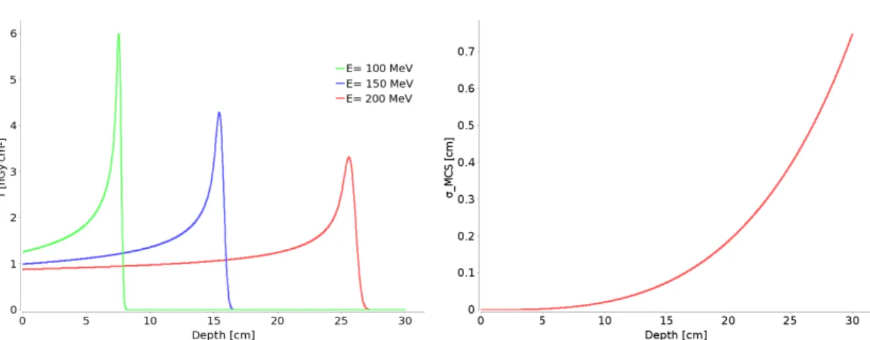
Bragg peak The integral dose distribution (T) from a quasi mono energetic beam measured in a water tank is called the Bragg peak. T is the integrated dose in an infinite plane at a single depth in water and therefore has the units Gy cm². The Bragg peak can be explained by the Bethe-Bloch-formula given above. Example Bragg peaks as used in the PSI treatment planning system for three different energies are shown in figure1.2.

From these integral depth dose curves the therapeutic benefit of protons for radiation therapy becomes apparent. Due to the Bragg peak most dose is deposited at the end of the beam range and almost no dose is deposited behind the Bragg peak. This is especially favorable compared to photon radiation, which deposits dose throughout the whole patient exposed to the beam. The proton beam energy determines the depth of the peak, whilst the width of the peak in beam direction is caused by range straggling and the beam energy spread. Range straggling increases in depth and thus deeper Bragg

(17)

4 1. Introduction

Figure 1.2: Integral dose T for three different energies (left) and beam width due to Multiple Coulomb Scatteringσ_MCS (right) as function of depth in water.

Figure 1.3: The spread out Bragg peak (red) is the sum of pristine Bragg peaks (blue) with different energies weighted such that a uniform dose in water depth is achieved.

peaks are wider. The beam proximal to the peak, where the dose is approximately flat is called the plateau region, which is well visible for the 200 MeV peak shown in figure 1.2. There the effect of the decrease in number of primary protons in the beam due to nuclear interactions and the effect of the increasing stopping power, because the protons slow down, cancel each other out. In this region the secondary particles from the nuclear interactions add a significant contribution to the dose. As such, the goal in radiotherapy to uniformly deliver dose to a multiple centimeter large target, cannot be met by a single Bragg peak, nor multiple Bragg peaks with lateral spacing. To achieve a homogeneous dose distribution in depth, therefore one has to add up multiple Bragg peaks with different energies and weights (figure1.3). This is called a spread out Bragg peak.

Dose Proton radiation at therapeutic energies (10-300 MeV) is ionizing. This means that upon collision with matter protons can knock electrons out of the shells of the target material. Although most of the energy will be deposited as heat, the ionizing characteris- tic of this radiation causes the damage, by creating free radicals in cells or directly hitting macromolecules such as DNA. The radicals and damage to DNA molecules can lead to cell death. The energy absorbed per unit target mass is called the physical absorbed

(18)

1.3. Pencil beam scanning 5 dose and is given by

D= dE dm =φS

ρ[Gy= J

kg], (1.3)

in units Gray. φis the proton fluence, defined as the number of protons crossing the infinitesimal area normal to the proton beam of the regarded test volume. This, multiplied with the mass stopping power, yields the absorbed dose. The damage caused by ionizing radiation and therefore tumor control probability and normal tissue complication depend on the absorbed dose.

Linear Energy Transfer LET of a material is the energy loss of an incident proton due to electronic interactions in traversing a distance dldivided by this distance.

LET = dE_∆

dl (1.4)

Similar to the stopping power, LET is highly energy dependent and increases for slower protons. For a proton beam incident on a water tank LET will therefore increase in depth until the protons stop. LET determines the ionization density along the trajectory of a proton, which can potentially affect how much biological damage is caused in the tissue.

Relative Biological Effectiveness In radiation therapy different particles cause different severity of damage in tissue. Therefore the concept of biological dose was introduced.

D_bio=D_phy∗RBE (1.5)

The relative biological effectiveness (RBE) is defined as the ratio between a dose from a reference modality (e.g. ⁶⁰C gamma radiation or photons from a linear accelerator) to a dose from the particle under surveillance, here protons, to achieve the same biological effectζ (e.g. cell survival or tumor control).

RBE := Dref

D_proton ζ=ζ0

(1.6) RBE is not a fixed value for a certain radiation modality and displays strong variations as a function of biological endpoint, dose, linear energy transfer and examined cell line [11]. Nevertheless in clinical practice for protons a fixed RBE value of 1.1 is used [12].

1.3 Pencil beam scanning

Proton therapy was first introduced with a scattered beam technique, similar to established photon therapy delivery techniques. However, the charge of the protons allows for scanning of the beam with scanning magnets. In 1996 the first patient was treated with pencil beam scanning (PBS) [13]. Scanning a relatively small proton beam, henceforth referred to as a pencil beam or a spot, through the target, allows for a better dose con- formation to the proximal target edge compared to a scattered beam. Hence, the target dose is delivered to the patient by thousands of individual pencil beams, which are placed in a grid covering the tumor. The interaction depth of each beam is adjusted by changing the energy of the protons. This can be achieved with a energy degrader upstream of the gantry. The lateral scanning of the pencil beams is achieved by so called scanning

(19)

6 1. Introduction magnets, which deflect the beam upstream of the patient such that the Bragg peak of the beam reaches the planned position. As such, pencil beam scanning does not require patient or field specific hardware (i.e. collimator or range compensator). The reduced amount of patient and field specific hardware in the beam close to the patient (especially if a energy degrader is used) significantly lowers the neutron contamination of the beam.

This together with the better dose distribution shaping capability of PBS compared to scattered beam techniques, makes PBS the state of the art delivery technique for proton therapy.

There are also certain drawbacks with PBS however. The method requires highly accurate delivery machinery, since it is very sensitive to spot position errors. Additionally patient motion with a similar speed as the scanned proton beam may cause large interplay effects [14].

1.4 Treatment workflow at PSI for Gantry 2

1.4.1 Treatment planning

Radiotherapy aims at treating the patient by delivering enough dose to the tumor to control it, while minimizing normal tissue complications. Controlling the parameters of the treatment and consequentially calculating the resulting dose distribution such that it fulfills the treatment goal, is called treatment planning. First, a planning computed tomography (CT) image of the patient in the treatment position is obtained. In this CT image the volumes of interest (VOI, e.g. target and organs at risk) are delineated, planning goals are established by a medical doctor and necessary margins are chosen by a medical physicist. At PSI an in-house developed treatment planning system (TPS) employing an analytical ray-casting algorithm for dose calculation is used [15]. In the TPS the delineated target and the corresponding margins can be displayed in the CT image. Then, the planner chooses the number of fields and incident directions. From this information a set of spot positions on a grid aligned with the field direction and covering the target are defined. In pencil beam scanning, the fluence of all these spots can be adapted individually, with the optimization of these weights being performed in the treatment planning software, such that the dose meets the treatment objectives.

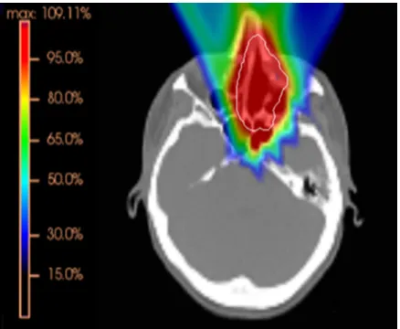
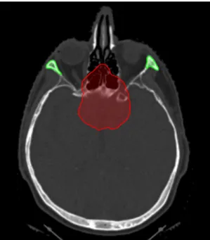
After optimization the dose distribution is calculated and evaluated. An example dose distribution of a three field plan covering a target in the nasopharyngeal region is depicted in figure1.4.

SFUD and IMPT Conceptually there are two different approaches for optimizing the spot weights. One is the single field uniform dose (SFUD) optimization. In SFUD all spot weights of one field are optimized simultaneously to achieve a homogeneous dose inside the target. Therefore such fields have dose gradients mainly at the edge of the target volume. This approach has some advantages considering robustness as is discussed in section1.7.1.

The other approach is called intensity modulated proton therapy (IMPT) [16]. With this technique all the spots of all the fields are optimized simultaneously aiming again for uniform target coverage, but also additional constraints to OARs can be entered into the optimization algorithm. This results in non uniform dose distributions of the single fields. Only the sum of the fields displays a homogeneous target coverage. IMPT allows for improved sparing of OARs, but due to dose gradients in single fields inside the target, robustness to delivery uncertainties is decreased.

(20)

1.4. Treatment workflow at PSI for Gantry 2 7

Figure 1.4: Color wash of an optimized dose distribution of a three field plan covering a target (displayed in white) in the nasopharyngeal region. The color bar indicates percentage of prescription dose.

1.4.2 Patient specific quality assurance and steering file evolution

Before treatment the information contained in the plan (e.g. spot positions, proton fluences or spot energies) is translated to a machine readable file, the steering file. The next step in the workflow is called steering file evolution. This process is specific to PSI and closely linked to delivery machine characteristics [17]. Other centers however, have similar steps in their workflow. The steering file evolution includes a scaling of the proton fluences to account for nuclear interactions, which are not entirely considered in the analytical dose calculation. This scaling factor originates either from measurements with the same setup as for the patient specific verification measurements or from an empirical model, which estimates these factors based on plan parameters. Further, the steering file evolution includes a measurement of the spot position deviations from the expected positions and consequent correction of those positions are written to the steering file. This process is internally called "teaching". Finally, an absolute dose measurement in a water phantom for at least one depth is obtained for every field. This last step is called patient specific verification. If the measurement is within some clearly defined clinical margins (see chapter 5) the steering file is ready for delivery. This steering file evolution and the patient specific verification measurements are time consuming and represent a bottleneck in the clinical workflow.

These verification measurements are not done for every fraction but only once per field. So the correct and reproducible performance of the delivery machine needs to be relied on. Therefore different regular machine quality assurance tests are performed within different intervals, including a daily check before treatment start.

(21)

8 1. Introduction

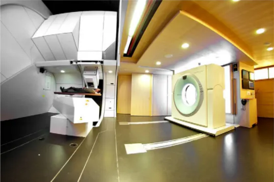
Figure 1.5: PSI Gantry 2 treatment room. On the left you can see the couch and a patient lying on it. Above is the gantry and the nozzle is pointing toward the patient.

On the right the CT on-rails is visible. (Picture from: Newsletter of the Center for Proton Therapy, Paul Scherrer Institut, October 2013, #1)

1.4.3 Delivery

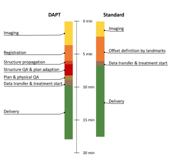
The treatment room with the couch, the CT on-rails and the gantry are depicted in figure 1.5. The daily treatment starts with the positioning of the patient on the couch with the help of fixation equipment (e.g. mask, bite-block) and positioning lasers. Then, a CT-on- rails is used to obtain 2D positioning scouts, which are compared to previously calculated projections of the planning CT, so called radiographs. With the help of manually drawn landmarks, offsets between the scouts and the radiographs are determined. These offsets are then sent to the delivery machine and the couch is moved to the treatment start position. Finally the delivery is started. The duration of the delivery strongly depends on the size of target and the number of fields and usually takes between 5 and 20 minutes.

For example a standard treatment plan with three fields to a target volume of 0.2 l can be delivered in about 8 minutes excluding patient set-up and positioning. During the delivery beam parameters of every spot are measured by the treatment verification system with the help of detectors in the treatment machine snout. These values, which are monitored during the delivery, are written in a so called log-file. If however the measured spot position or fluence is outside of specific safety limits, the treatment is interrupted.

1.5 Algorithms

1.5.1 Dose calculation algorithm

The analytical dose calculation algorithm for proton therapy as used at PSI was developed by Scheib in 1993 [18]. A beam model is defined by the integral depth dose curve T(s)

(22)

1.5. Algorithms 9

and the width of the lateral distribution σ(s) as a function of depth s. This data can either be obtained by measurements, by calculations or a combination of both. The dose to a point delivered by a single pencil beam in water can now be expressed as

D(s, t, u) = T(s) 2πσ_t(s)σ_u(s)e⁻

t2 2σ2

t(s)e⁻

u2 2σ2

u(s), (1.7)

where t and u are the lateral distances to the pencil beam axis. The width of the beam due to MCS and the initial angular-spatial distribution (IASD) is given by

σ_t,u(s)² =σ²_{M CS}(s) +σ_IASD,t,u² (s). (1.8) To calculate the dose in patient geometries, the water equivalent depth for every voxel has to be determined. The CT voxel data, which is given in Hounsfield units (HU) needs to be converted into relative proton stopping power. This is done using CT specific lookup tables. Despite regular checks of these lookup tables there is an inherent uncertainty in this conversion, due to the different interactions of protons and photons, which are used to obtain the CT. The resulting range uncertainty will be discussed in section1.7.1. After the conversion, the water equivalent path length given a field direction can be calculated with an algorithm as described by Siddon [19]. The ray along the field direction to the regarded point is segmented according to the voxels and scaled with the voxels stopping power. The dose distribution in a patient geometry with the ray casting algorithm as proposed by Schaffner et al. [15] for the j^th spot is now given by

Dj(s, t, u) = T(w)

2πσt(w)σu(w)e⁻

(t−tj)2 2σ2

t(w)e⁻

(u−uj)2 2σ2

u(w) , (1.9)

where s is substituted by the water equivalent depth w(s, t, u). For a point away from the beam axis, w might differ from the point on the beam axis because of density heterogeneities.

The overall dose of a field consisting of multiple thousand spots is given by the summation of the spot contributions multiplied by the weight ωj of the corresponding spot j.

D_tot(s, t, u) =

M

X

j=0

ω_jD_j(s, t, u) (1.10)

A different way to put it is, the total dose vector D (all dose values at the evaluation points) can be written as

D=d ω, (1.11)

whereω is the weight vector and d is the dose deposition matrix. d has dimension of number of evaluation points multiplied by the number of spots.

1.5.2 Spot placement and target definition

During the plan generation, for a given field direction and target structure a set of spots is chosen, which are subsequently optimized. The spots lie on a grid, which is aligned with the field direction. The lateral spacing of the grid is 4 mm and the spacing along the beam direction is 5 mm for spots with a water equivalent depth above 12.5 cm and a spacing of 2.5 mm otherwise. All points on this grid, which lie in the target structure

(23)

10 1. Introduction or have a distance of 3 mm to the target, are included in the optimization. The planned dose P is chosen to be homogeneous inside the target and has a Gaussian fall-off at the edges. Finally an importance function g, used for plan optimization, is also defined, which is homogeneous inside the target, and has an exponential fall-off at the edges.

1.5.3 Optimization algorithm

A cost function describing the difference of the dose distribution to the planned dose as a function of the weight vectorω can be defined as follows:

F(ω) =

N

X

i

g²(P_i−D_i)² (1.12)

Here N denotes the number of voxels, gi is the importance function (see above), Pi

is the planned dose andD_i is the calculated dose of thei^thvoxel. The cost function can be minimized by iteratively adapting the weights with the update function as described by Albertini et al. [20]:

ω_j(k+ 1) =ω_j(k) P

ig²_id²_ij(k)_D^Pⁱ

i(k)

P

ig²_id²_ij(k) , (1.13) where d_ij is the dose contribution of the j^th spot to the i^th voxel. This is a quasi Newtonian step function using a damping factor describing the contribution of a spot to a certain voxel in relation to the total dose at this voxel as proposed by Lomax et al.

[21].

Optimizing the weights of all spots of one field results in an SFUD plan. If all spots of multiple fields are optimized simultaneously this results in an IMPT plan. This involves accumulating the dose of the different fields in every iteration. The PSI treatment software allows for additional dose constraintsΠ_l to organs at risk (OAR) l in the case of an IMPT plan. The update function becomes

ωj(k+ 1) =ωj(k) P

i

g_i²d²_ij(k)_D^Pⁱ

i(k)+POAR

l H(Di(k),Π_i,l)γ_i,l²d²_ij(k)_D^Π^l

i(k)

P

i

g²_id²_ij(k) +POAR

l H(Di(k),Π_l)γ_i,l² d²_ij(k)

, (1.14)

where γ_i,l is the importance value of the OAR l. This importance value is given relative to the target, which has importance 1. The function H is a step function and turns the constraint voxelwise on and off, depending on if the constraint is fulfilled considering that specific voxel.

H(D_i(k),Π_l) =

0,(i /∈l)∨(Di(k)<Π_l)∨(Di(k)> D@V C_l)

1, otherwise (1.15)

Here,D@V C_l stands for the dose at volume constraint of organ l.

Finding suitable importance values for the OARs is a manual process done during planning. Since the size of the OAR is not considered in the optimization, often for small OARs a higher importance value needs to be chosen, such that the treatment goal is fulfilled. Currently, this process relies on a trial and error approach during the plan generation.

(24)

1.6. Conformity and robustness 11

1.6 Conformity and robustness

As mentioned earlier, the goal of radiation therapy is to deliver a homogeneous dose to the target and no dose to the surrounding tissue. This goal will be referred to as conformity. There are different limitations to this goal of conformity. The most obvious limitation comes from the physical characteristics of the therapeutic beam (e.g. depth dose curve, lateral and distal penumbra). Critical structures in proximity of the target (e.g. OAR) add additional difficulties to the planning process. Clearly, therapy modalities, which are able to apply sharp dose gradients allow the creation of more conformal plans. However in clinical practice, conformity is not the only requirement to the plan.

The plan should be robust as well. Plan robustness is the preservation of the planning goals (e.g. minimum dose to target or maximum dose to OAR) in the presence of uncertainties. The requirement for robustness often adds a higher limitation to conformity than the limitations from the beam characteristics.

The sharp distal and lateral dose falloff of proton beams enable the generation of dose fields with steep gradients. Especially for IMPT plans, such steep gradients can be located even in the middle of a target or in close proximity to OAR. While this, as already suggested, has benefits for creating conformal plans, the steep dose gradients greatly diminish robustness [22]. Therefore managing uncertainties and understanding the consequences of these uncertainties to conformity and robustness is very important for proton therapy.

1.7 Uncertainties and managing uncertainties

1.7.1 Uncertainties

Target identification Target identification uncertainties are basically the first source of uncertainties in the treatment process. The accuracy of gross target volume (GTV) delineation is closely linked to the imaging modality. Increased resolution of CT and MRI as well as new PET tracers eliminate some of the uncertainty [23], but inter and intra observer variability remains [24]. These uncertainties are usually in the order of a few millimeters. In the surrounding tissue of the tumor there is a high chance for microscopic tumor extensions, which are not visible with current imaging techniques [25]. This problem is usually addressed by extending the target to the clinical target volume (CTV). The amount of this extent is usually based on histopathological studies and the clinician’s experience [25]. The extension margin basically determines the local recurrence probability and has inherently a high uncertainty. Up to now, uncertainties from other sources called for a reduction in the conformity of the radiotherapy plan.

This entailed dose deposition to the area around the CTV. If by new technology these uncertainties are reduced, which would allow for more conformal plans, there is the risk that due to uncertainties in CTV extension margins, the risk of local recurrence increases [25].

Machine uncertainty Machine uncertainty depends on the treatment modality as well as the delivery machine itself. It is important to know how precise a machine can deliver dose, since this puts the other uncertainties in perspective. Here, some parameters of the proton Gantry 2 at PSI will be given. The pencil beams inside the patient have a lateral spot size with full width at half maximum between 1 and 4 cm depending on the energy and depth in the patient [13]. The lateral spot position accuracy is below 1.5 mm.

(25)

12 1. Introduction For higher deviations an interlock is triggered. However, for most spots the accuracy is below 0.5 mm. The energy tuning uncertainties are about 0.1 %, which converts to a range error in water equivalent depth of below 0.5 mm [13]. However, for a low density target, like the lungs, the uncertainty in range can increase substantially.

Dose calculation Dose calculation has an inherent uncertainty. The dose is calculated in the patient CT and errors in this CT data will obviously influence the dose calculation.

Error sources in the CT data are artifacts from metal implants, noise in the measurement (more prominent for low dose CT) or effects from beam hardening. For dose calculation the Hounsfield units (HU) as measured in the CT need to be converted to proton stopping power. At PSI a biologically verified conversion curve is used [26]. Errors from this conversion were measured in biological samples and determined to be around 1 % for soft tissue and 2 % for bone [27]. Combined with errors in the acquisition of the CT data HU uncertainty of ±3% should be considered [28]. This will translate almost directly to uncertainty in range, so the position of the Bragg peak of a pencil beam might be off by up to 3 % of its range. Additional, errors arise from the dose calculation itself, because the analytical algorithm is only an approximation of the whole reality of the dose deposition. The gold standard for dose calculations are Monte Carlo (MC) simulations.

Behind density heterogeneities voxel by voxel comparison between Monte Carlo dose engines and analytical calculations show differences of up to 15 %. In normal situations however, for 90% of the voxels the differences are below 5% [28].

Patient motion Patient motion can be divided into intra-fraction and inter-fraction motion. Intra-fraction motion are movements of the patient or parts of the patient, happening during the time when the patient lies on the couch and a treatment is delivered.

Examples for this motion are breathing, swallowing, the heart beat or a small shift of the patient on the couch. The latter effect is minimized by immobilization techniques like head masks or bite-blocks. The other intra-fraction motions strongly depend on the target location inside the patient and can sometimes partially be mitigated by smart choices of field directions. The size of these uncertainties are well reported [29] and there are many techniques under investigation on how to tackle this problem of intra-fraction motion, which will not be further discussed.

Inter fraction motion are changes in the patient between different fractions, so from day to day. One source are daily set up differences. These set-up errors depend on the immobilization modality and are well reported. For head and neck patients for example head masks are often used for immobilization and a set-up uncertainty with a standard deviation of 0.95 mm is reported [30]. The other sources are anatomical changes. Examples are changes in patient weight [31], deformation and displacement of internal organs due to changes in bladder and rectal filling [32] or mucus filling variations [33]. Anatomical changes can have a large impact on proton dose distributions [34].

Conflicting objectives of radiation treatment Conflicting objectives of radiation treatment raise big challenges in the planning process and cause uncertainties as well.

Examples of such conflicting objects are minimum dose constraints in the target with absence of hot spots, sparing of OAR, increasing robustness and reducing the number of fields or spots to decrease treatment time. A lack of well established dose–response relationships between dose maps and the probability of various clinical outcomes make optimal balancing between the conflicting objectives challenging. Additionally, the available dose-response relationship data comes mostly from photon therapy, but the estab-

(26)

1.7. Uncertainties and managing uncertainties 13

lished 1.1 RBE conversion factor has some uncertainty itself. Still the clinician has to decide on a treatment plan, relying on estimated dose response relationships and his/her experience. The degeneracy of this decision however is a cause for uncertainty [35].

Range uncertainty Range uncertainty is a much discussed topic in proton therapy.

This is due to the sharp distal dose gradient as discussed above. Additionally, uncertainty in lateral spot position in the presence of density heterogeneities can cause a range uncertainty, which may even exceed the original lateral error in severity. One could make the point that in proton therapy it is needless to distinguish between range uncertainty and general uncertainties. Accordingly, the previous paragraphs summarize sources for range uncertainties. The highest absolute values for range deviations are due to anatomical changes and CT artifacts, which in worst case scenarios account for errors in the centimeter range. Distal end RBE enhancement and inherent CT uncertainties (e.g. beam hardening, and HU to stopping power conversion) contribute to additional uncertainties for up to a few millimeters. Additionally patient positioning and uncertainties in the beam energy have the smallest, but a not negligible contribution to range uncertainty.

Different mitigation strategies, employed to assure a safe treatment in presence of such uncertainties, will be discussed in the following section.

1.7.2 Managing uncertainties

Systematic and random errors When regarding the clinical consequences of uncertainties, one has to distinguish between random and systematic errors. Due to fraction- ation of the treatment random errors cause a smearing out effect of the planned dose [20]. This reduces conformity of the plan, but there is no need for a plan to be robust to a single random error scenario. Therefore, establishing a robust plan for worst-case random errors might be over conservative at the cost of conformity. Also when regarding multiple sources of random errors one does not need to add the errors up linearly but using a root mean sum. On the other hand, systematic errors will ad up linearly, and a worst case approach is necessary because the same error might be present in every fraction, worsening the under or over dosage due to the error further and further. Most uncertainties have a random and a systematic contribution. For proper consideration of the uncertainties these need to be separately determined.

PTV The most common way to handle uncertainties in photon therapy is the extension of the CTV to the planning target volume (PTV) [36, 37]. There are some difficulties with directly adopting this method to proton therapy. The sharply defined Bragg peak, dose gradients within a field and the resulting sensibility to range uncertainties, yield an additional source for differences between the planned and the delivered dose [38]. Many proton therapy centers using spot scanning techniques discarded the PTV approach and decided to deal with the uncertainties with a robust optimization approach, as described in the following paragraph. On the other hand, other centers, including our own, have retained the PTV approach due to drawbacks with current robust optimization imple- mentations. This approach itself gives no robustness guarantee however and robustness needs to be carefully surveyed for every plan. The possibility to steer the optimization result to a more robust solutions by tweaking the starting conditions of the optimizer is described [39] and might be necessary for certain situations.

(27)

14 1. Introduction Robust optimization Robust optimization is the alternative to using a PTV, whereby error scenarios are directly incorporated into the optimization algorithm as proposed by Unkelbach et al. [40]. The considered scenarios can include setup errors, HU to stopping power conversion uncertainties and/or different anatomical situations [41]. There are different optimization approaches. One is to optimize the objective functions on the worst-case situation and thereby minimize the impact of the uncertainties on these objectives. Another is the all scenario robustness, where all error scenarios are optimized simultaneously [42]. However, to achieve adequate CTV coverage under consideration of different error scenarios, especially in the case of worst case optimization, the initial plan conformity is decreased [40]. Hence, more sophisticated algorithms including robustness in a multi-criteria optimization based on "minimax" algorithms have been introduced [43]. With this approach it might be easier to investigate the difficult trade-offs between robustness and conformity.

Field direction Due to range uncertainty, the lateral penumbra is often preferentially used to provide a dose gradient between the target and OARs. This approach improves the robustness of a plan, since otherwise the OAR might easily move into the high dose area due to range uncertainty. Additionally, the severity and likelihood of inter- and intra-fraction patient motion need to be estimated. Therefore choosing field directions, which do not go through changing structures or which are perpendicular to expected organ motion can improve robustness as well.

Image Guided Radiotherapy IGRT is an umbrella term including any kind of adaptive radiotherapy (ART) and online positioning correction procedures. Here, IGRT will be used for correcting positioning errors of the patient and ART will be used for more complex plan adaption like correcting for anatomical changes. The realization of positioning correction depends on the available imaging modality in the treatment room. 2D to 2D matching of daily to reference radiographs has been the historical standard in proton therapy. But with increasing availability of in room 3D imaging modalities, such as cone beam computed tomography (CBCT) or in-room CT on-rails, 3D to 3D mapping is also used for patient positioning. Furthermore, both online and offlinee imaging and correction protocols can be used. For offlinee correction the positioning errors are recorded over the course of the treatment and if a systematic error in positioning is detected, this is corrected for. For the online case, the errors are corrected for before every treatment, reducing the systematic and random positioning errors. For example, the effect of online CBCT guided correction in IMRT for nasopharyngeal cancer was reported to allow for a reduction of PTV margin from 5-6 mm to 3 mm [44].

Adaptive radiotherapy At the moment adaptive radiotherapy is mainly employed for indications where anatomical or tumor changes have a big impact on the dose distribution. The current standard procedures depend on the indication and also on the practice of the treatment center. For plans which are critical in respect to anatomical changes, regular control imaging is inevitable [45]. If the changes in the patient and the resulting changes in the dose distribution are above a certain threshold, this triggers a re-planning process [46]. Another approach are plan of the day strategies [43]. This means that different plans are prepared for different anatomical scenarios (e.g. nasal cavity filling level). Before treatment, the patient is imaged and the scenario most similar to the current situation is chosen and the corresponding plan applied. This plan of the day strategy is very labor intensive and covering all anatomical scenarios is difficult.

(28)

1.8. Aim and outline of this thesis 15

A more universal approach is an online adaptive approach, where the plan is adapted according to the information from the pre-treatment image. Daily online adaption has many benefits and challenges as will be discussed in the following chapter.

In vivo range verification As discussed in section 1.7.1 in proton therapy range deviations are the main contributors to differences in planned and applied dose. So by verifying the range of the protons in vivo the differences could be corrected for. There are offlinee and online approaches for this range verification. As for IGRT, online approaches may enable a much larger benefit for the patient as the offlinee approach. Examples of range verification modalities are implanted range probes, proton radiography, prompt gamma imaging, PET [47] and MRI imaging [48]. However up to now either the ef- fort necessary to apply these measurements or the corresponding measurement accuracy (depending on the modality around 3 mm [49]) have prevented these techniques to be deployed in clinical practice.

1.8 Aim and outline of this thesis

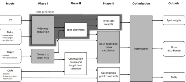
This thesis focuses on tackling the problem of inter fraction patient motion (e.g. anatomical changes and positioning errors) by online plan adaption. We call the technique Daily Adaptive Proton Therapy (DAPT). The technique is tailored to anatomical regions and indications, where we expect little deformations for the target and the OAR structures (e.g. the head). In the following chapter first, the generic approach of online adaption in proton therapy is summarized and the relevant literature reviewed (chapter2). Following this literature review, the next four chapters are published papers (three are published and one is in the submission process), which all directly cover topics related to online adaption in proton therapy. In this thesis, either the content of the published version or a pre-print version of the papers is added. Additionally, at the end of each of these papers a "summary and context" section has been added to give the reader the context of how the chapter fits in the big picture and to link the chapters together. The first of these chapters describes the workflow and the implementation we developed for DAPT at PSI (chapter 3). This work brings together the main findings of this PhD and describes the specific solutions for DAPT at PSI. The following three chapters detail specific problems of online adaption in proton therapy. These are ordered according to the appearance of the problem in the DAPT workflow. First, the question: "How can we speed up the plan generation step, such that we can use it for plan adaption in DAPT?" is addressed (chapter 4). Second, the question "How does a measurement free patient specific verification compare to the standard verification measurements and is it safe to omit the measurements for DAPT?" is investigated (chapter 5). And finally, the question:"Can we use the information of previous DAPT deliveries to refine the daily one?" is discussed (chapter6). For ease of navigating this thesis, figure1.6shows how chapters 3-6 fit in the workflow. PSI specific challenges for the DAPT workflow are addressed in the appendix.

(29)

16 1. Introduction

Figure 1.6: Thesis navigation aid: A simplified scheme depicting the DAPT workflow is shown. How the published papers (Chapter 3-6) fit in the DAPT workflow is indicated by the arrows and for each the main research question is stated.

(30)

2 | Daily adaptive proton therapy

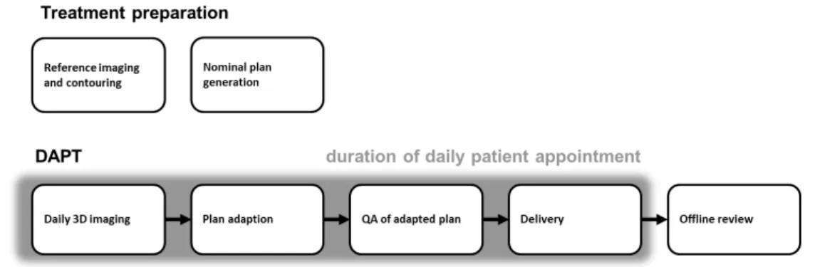
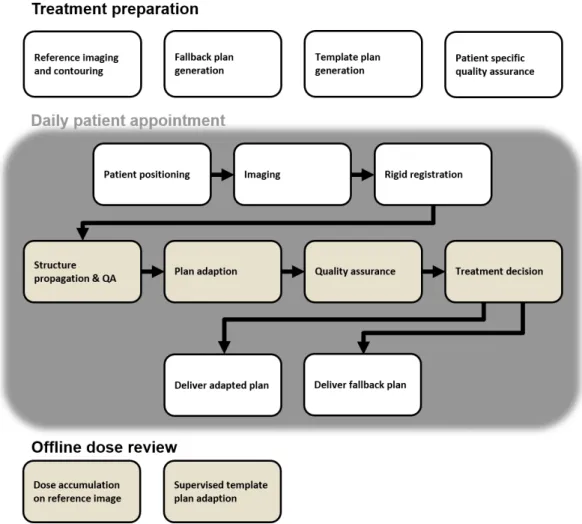
Daily adaptive proton therapy (DAPT) is an approach to tackle the problem of inter fraction patient motion. The goal is to decrease uncertainties due to inter fraction anatomical changes and patient setup errors, which in return allows for the delivery of a more conformal plan. A generic schematic depicting the concept of DAPT can be seen in figure 2.1. Treatment preparations analog to a standard treatment are conducted: A planning CT is taken, a reference plan is generated and usual quality assurance steps are executed. This is done days before treatment start. The procedure of the consecutive daily treatments is always the same. The patient is positioned and imaged in the same position as for the planning CT. While the patient remains immobilized on the couch, the plan is re-optimized on the daily image. In this step the reference plan is used as a starting point for the re-optimization. This facilitates the daily plan generation, since it needs to be fast. Before the newly generated daily plan can be applied, quality assurance (QA) checks, which guarantee a good plan quality and a flawless delivery, need to be conducted. After the delivery a thorough offline dose review might be advisable, since there was only limited time to check the adapted plan beforehand.

The so far mentioned steps for DAPT are generic. The problems and current research status of DAPT will be discussed in more detail in the following sections. The chapter is structured following the above described workflow and by the review article by Albertini et al. [50].

2.1 Treatment preparation

For the DAPT concept, the steps of reference imaging, diagnostics and drawing the con- tours on the planning CT remain unchanged. A reference plan first needs to be generated.

One of the most important steps in the reference plan generation is the determination

Figure 2.1: The schematic work flow diagram of a generic daily adaptive proton therapy treatment.

17

(31)

18 2. Daily adaptive proton therapy of the field incident angles. This is done manually and requires a lot of experience. For standard therapy, positioning uncertainties and inter-fraction anatomical changes need to be considered. For example, beam directions are typically avoided if they pass areas where large anatomical changes are expected. However, for the reference DAPT plan, no such restrictions need to be considered, since day-to-day changes in anatomy can be automatically corrected [51]. Additionally, margins to ensure target coverage under positioning uncertainties can be reduced. The reference plan for DAPT however still needs to be robust to HU to stopping power translation uncertainties, structure propagation uncertainties and couch motion uncertainties. So, the difference between generating a reference plan for DAPT and for standard treatments are different robustness demands.

A conservative approach could be to take the same plan for a DAPT reference as for standard treatments, but DAPT would also allow for a margin reduction and the choice of anatomically unrobust field angles. Unfortunately, there is only little literature available about how the new online adaption concept for protons changes the reference plan generation approach, since, as far as we are aware, currently there are no centers who treat patients with DAPT.

2.2 Daily imaging

From the DAPT methodology clear requirements to the 3D daily imaging modality emerge. First, one needs to be able to calculate a new plan on the anatomy visible in the image. This means that a high resolution proton stopping power map needs to be extracted from the image. Additionally, either the relevant OARs and the target need to be visible on the image or an accurate registration between the daily image and the reference image needs to be possible. Second, to get rid of positioning errors, the patient cannot be moved between the daily image and the consecutive treatment. This limits the imaging modality to in room devices. Third, dose contribution from the imaging process is highly critical since the process is repeated on a daily basis. Currently, there are three imaging modalities capable of fulfilling this requirements: Computed tomography (CT), cone beam CT (CBCT) and magnetic resonance imaging (MRI).

The big benefit of MRI is the high soft tissue contrast and the absence of imaging dose [52]. This is the reason that currently the biggest advances in adaptive radiotherapy are made with MR-Linac systems. For DAPT however, there are three major problems:

It is difficult to convert the MRI image to a proton stopping power map, the accelerated protons interact strongly with the magnetic field of the MR system [53] and the magnetic fields of the proton beam line can also disturb the imaging system. There is a lot of promising research going on to tackle these problems. With deformable image registration (DIR) atlas based stopping power maps can be warped on to MR images [54,55,56,57] or with the help of machine learning algorithms information from different MR sequences can be translated directly to stopping power [58, 59]. Currently however, for proton therapy MR-only planning is not yet applied in clinical practice.

The use of CBCT for adaptive proton therapy is widely discussed. The main advantages of CBCT are the little space necessary in the treatment room and the small dose contribution, which is roughly fifteen time less than a conventional multi-slice CT [60].

On the other hand, HU values from CBCT can not be easily calibrated and hence one can not plan on the resulting image. Different centers are working on circumventing that problem [61,62,63,64,65]. Similar to MR-based planning, the idea is to use deformable image registration to map the HU values of a planning CT on to the daily CBCT. The drawbacks are the inherent uncertainties of DIR and a lack of easy and automated quality