Synoptic analysis of a decade of daily measurements of SO 2 emission in the troposphere from volcanoes of the

(1)

https://doi.org/10.5194/essd-13-1167-2021

Synoptic analysis of a decade of daily measurements of SO ₂ emission in the troposphere from volcanoes of the

global ground-based Network for Observation of Volcanic and Atmospheric Change

Santiago Arellano¹, Bo Galle¹, Fredy Apaza², Geoffroy Avard³, Charlotte Barrington⁴, Nicole Bobrowski⁵, Claudia Bucarey⁶, Viviana Burbano^7,, Mike Burton^8,a, Zoraida Chacón⁷, Gustavo Chigna⁹, Christian Joseph Clarito¹⁰, Vladimir Conde¹, Fidel Costa⁴, Maarten De Moor³,

Hugo Delgado-Granados¹¹, Andrea Di Muro¹², Deborah Fernandez¹⁰, Gustavo Garzón⁷, Hendra Gunawan¹³, Nia Haerani¹³, Thor H. Hansteen¹⁴, Silvana Hidalgo¹⁵, Salvatore Inguaggiato⁸,

Mattias Johansson¹, Christoph Kern¹⁶, Manne Kihlman¹, Philippe Kowalski¹², Pablo Masias², Francisco Montalvo¹⁷, Joakim Möller¹⁸, Ulrich Platt⁵, Claudia Rivera^1,b, Armando Saballos¹⁹, Giuseppe Salerno⁸, Benoit Taisne⁴, Freddy Vásconez¹⁵, Gabriela Velásquez⁶, Fabio Vita⁸, and

Mathieu Yalire²⁰

1Department of Space, Earth and Environment, Chalmers University of Technology, Gothenburg, Sweden

2Instituto Geológico, Minero y Metalúrgico (INGEMMET), Arequipa, Peru

3Observatorio Vulcanológico y Sismológico de Costa Rica (OVSICORI), Heredia, Costa Rica

4Earth Observatory of Singapore (EOS), Nanyang Technological University, Singapore

5Institute of Environmental Physics, Heidelberg University, Heidelberg, Germany

6Servicio Nacional de Geología y Minería (SERNAGEOMIN), Temuco, Chile

7Servicio Geológico Colombiano (SGC), Bogotá, Colombia

8Istituto Nazionale di Geofisica e Vulcanologia (INGV), Rome, Italy

9Instituto Nacional de Sismología, Vulcanología, Meteorología e Hidrología (INSIVUMEH), Guatemala City, Guatemala

10Philippine Institute of Volcanology and Seismology (PHIVOLCS), Quezon City, Philippines

11Instituto de Geofísica, Universidad Nacional Autónoma de México (UNAM), Mexico City, Mexico

12Observatoire Volcanologique du Piton de la Fournaise, Institut de Physique du Globe de Paris (IPGP), Paris, France

13Center for Volcanology and Geological Hazard Mitigation (CVGHM), Bandung, Indonesia

14GEOMAR Helmholtz Centre for Ocean Research, Kiel, Germany

15Instituto Geofísico (IGEPN), Escuela Politécnica Nacional, Quito, Ecuador

16Volcano Disaster Assistance Program (VDAP), United States Geological Survey (USGS), Vancouver, WA, United States

17Servicio Nacional de Estudios Territoriales (SNET), San Salvador, El Salvador

18Möller Data Workflow Systems AB (MolFlow), Gothenburg, Sweden

19Instituto Nicaragüense de Estudios Territoriales (INETER), Managua, Nicaragua

20Observatoire Volcanologique de Goma (OVG), Goma, Democratic Republic of the Congo

anow at: Department of Earth and Environmental Sciences, University of Manchester, Manchester, UK

bnow at: Centro de Ciencias de la Atmósfera, Universidad Nacional Autónoma de México, Mexico City, Mexico

deceased

Correspondence:Santiago Arellano (santiago.arellano@chalmers.se)

(2)

Received: 1 October 2020 – Discussion started: 3 November 2020

Revised: 27 January 2021 – Accepted: 11 February 2021 – Published: 22 March 2021

Abstract. Volcanic plumes are common and far-reaching manifestations of volcanic activity during and between eruptions. Observations of the rate of emission and composition of volcanic plumes are essential to rec- ognize and, in some cases, predict the state of volcanic activity. Measurements of the size and location of the plumes are important to assess the impact of the emission from sporadic or localized events to persistent or widespread processes of climatic and environmental importance. These observations provide information on volatile budgets on Earth, chemical evolution of magmas, and atmospheric circulation and dynamics. Space- based observations during the last decades have given us a global view of Earth’s volcanic emission, particularly of sulfur dioxide (SO₂). Although none of the satellite missions were intended to be used for measurement of volcanic gas emission, specially adapted algorithms have produced time-averaged global emission budgets.

These have confirmed that tropospheric plumes, produced from persistent degassing of weak sources, dominate the total emission of volcanic SO2. Although space-based observations have provided this global insight into some aspects of Earth’s volcanism, it still has important limitations. The magnitude and short-term variability of lower-atmosphere emissions, historically less accessible from space, remain largely uncertain. Operational monitoring of volcanic plumes, at scales relevant for adequate surveillance, has been facilitated through the use of ground-based scanning differential optical absorption spectrometer (ScanDOAS) instruments since the be- ginning of this century, largely due to the coordinated effort of the Network for Observation of Volcanic and Atmospheric Change (NOVAC). In this study, we present a compilation of results of homogenized post-analysis of measurements of SO₂flux and plume parameters obtained during the period March 2005 to January 2017 of 32 volcanoes in NOVAC. This inventory opens a window into the short-term emission patterns of a diverse set of volcanoes in terms of magma composition, geographical location, magnitude of emission, and style of eruptive activity. We find that passive volcanic degassing is by no means a stationary process in time and that large sub-daily variability is observed in the flux of volcanic gases, which has implications for emission budgets produced using short-term, sporadic observations. The use of a standard evaluation method allows for intercom- parison between different volcanoes and between ground- and space-based measurements of the same volcanoes.

The emission of several weakly degassing volcanoes, undetected by satellites, is presented for the first time. We also compare our results with those reported in the literature, providing ranges of variability in emission not accessible in the past. The open-access data repository introduced in this article will enable further exploitation of this unique dataset, with a focus on volcanological research, risk assessment, satellite-sensor validation, and improved quantification of the prevalent tropospheric component of global volcanic emission.

Datasets for each volcano are made available at https://novac.chalmers.se (last access: 1 October 2020) under the CC-BY 4 license or through the DOI (digital object identifier) links provided in Table 1.

1 Introduction

Volcanic eruptions are to a large extent triggered or modu- lated by the intricate dynamics of segregation and escape of volatiles from magmas, making the observation of the rate of gas emission an important component of monitoring efforts to identify and predict the state of a volcanic system (Sparks, 2003; Sparks et al., 2012). The resulting atmospheric plumes are the farthest-reaching products of volcanic activity and constitute rich environments for a number of important processes affecting the physics and chemistry of the atmosphere, the radiative balance of the climate system, or the biogeo- chemical impact on soils and the ocean (e.g. Robock, 2000;

Langmann, 2014; Schmidt et al., 2018).

Volcanoes are sources of many trace atmospheric compounds, such as water vapour (H₂O), carbon dioxide (CO₂), sulfur dioxide (SO₂), carbonyl sulfide (OCS), hydrogen chlo-

ride (HCl), hydrogen fluoride (HF), hydrogen sulfide (H2S), and molecular hydrogen (H2), as well as solid particles and metals. From these species, SO2is the most widely observed by passive optical remote sensing methods (Oppenheimer, 2010). This is a consequence of its low atmospheric background and accessible radiation absorption bands, particularly in the near-ultraviolet (NUV) and mid-infrared (MIR) spectral regions. This is advantageous for several reasons, for example, for (1) the volcanologist, SO₂is a reliable tracer of magmatic activity due to its strongly pressure-dependent solubility in magmas. Since H₂O is usually the most abundant volatile species and thus the most important driver of volcanic activity and has a pressure-dependent solubility, both H₂O and SO₂ fluxes are positively correlated with eruptive intensity. For (2) the climatologist, SO₂may be transformed by a series of reactions into aerosols containing sulfuric acid (H2SO4), which exert a strong radiative forcing, especially

(3)

when reaching the stratosphere. Or, for (3) the meteorologist, SO₂has a long enough residence time in the atmosphere to serve as a tracer of volcanic plume transport at regional or even global scales.

Measurements of the mass emission rate or flux of SO₂ from volcanoes started in the 1970s with the development and application of the correlation spectrometer (COSPEC) (Moffat and Millán, 1971; Stoiber and Jepsen, 1973). This instrument disperses ultraviolet sky radiation using a grating and employs a mechanical mask to correlate the intensity of diffused solar radiation in the near-ultraviolet region at se- lected narrow bands, matching absorption features of SO2. With proper calibration using cells containing SO2at known concentrations, the COSPEC instrument measures the column density of SO2 relative to background by the methods of differential absorption. Flux is quantified assuming mass conservation: the volcanic source emission strength is equal to the integrated flux across a surface surrounding the volcano when no other sources or sinks are enclosed. The integrated flux is measured by scanning through a surface per- pendicular to plume transport, integrating the column densities in the plume cross section, and multiplying this integral by the corresponding transport speed. COSPEC was typically used for sporadic or periodical field surveys, during both volcanic crises and periods of passive degassing. The first global emission budgets for volcanic SO₂were based on extrapola- tion of these sporadic measurements on a fraction of glob- ally degassing volcanoes, through a series of non-verified assumptions regarding the statistics of emission for measured and non-measured sources. Halmer et al. (2002) recognized this problem and highlighted the need for increasing (i) the number of monitored volcanoes, (ii) the periods of observation, (iii) the sampling frequency of the measurements, and (iv) the homogeneity of protocols of measurement by different observers.

In the late 1970s, the first satellite-based sensors, intended primarily for monitoring the stratospheric ozone (O₃) layer, opened up the possibility of mapping and quantifying vol- canogenic SO₂ from space (Krueger, 1983; Krueger et al., 1995). The successful Total Ozone Mapping Spectrometer (TOMS) instrument programme was succeeded by a series of optical instruments such as the Global Ozone Monitoring Ex- periment (GOME/GOME-2), the Scanning Imaging Absorp- tion Spectrometer for Atmospheric Cartography (SCHIA- MACHY), the Ozone Monitoring Instrument (OMI), and the Ozone Mapping and Profiler Suite (OMPS). Infrared (IR) sensors, such as Infrared Atmospheric Sounding Interfer- ometer (IASI) or Moderate Resolution Imaging Spectrora- diometer (MODIS), have been also used for routine global observation of volcanic emissions (Khokhar et al., 2005;

Carn et al., 2013; Theys et al., 2013). More recently, the Tropospheric Monitoring Instrument (TROPOMI), on board ESA’s Sentinel-5 Precursor satellite since 2017, achieves a factor of 3 to 4 better sensitivity than OMI, due to better spatial resolution and sensor performance. This makes de-

tection of weak emissions of SO2 in the lower atmosphere feasible every day and with global coverage. Under ideal measurement conditions and knowledge of plume velocity, time series of volcanic SO₂flux as low as∼1 kg/s (for 1 m/s wind speed) with sub-daily frequency can be derived from TROPOMI (Queißer et al., 2019; Theys et al., 2019).

During the 1990s and early 2000s smaller, cheaper, and more accurate and versatile alternatives to the COSPEC instrument were developed, in particular the miniaturized differential optical absorption spectrometer (MiniDOAS) (Galle et al., 2003). This instrument incorporates a grating spectrometer to obtain the spectrum of diffused solar radiation in the UV (ultraviolet) spectrum and retrieves the relative column density of SO2by the DOAS method (Platt and Stutz, 2008). This line of research led to the implementation of fully automated scanning DOAS (or ScanDOAS) systems (Edmonds et al., 2003), which have enabled volcanological observatories to conduct nearly continuous monitoring of volcanic plumes. A version of this instrument, known as dual-beam scanning DOAS, can measure the plume velocity, height, and the integrated SO₂ flux in near to real time, with a time resolution of 1–15 min during daylight hours (Jo- hansson et al., 2009). Similar spectroscopic instruments have been developed or replicated by different groups (Horton et al., 2006; Mori et al., 2007; Arellano et al., 2008; Burton et al., 2008; Salerno et al., 2009).

Among other methods for ground-based optical remote sensing of integrated volcanic flux we highlight different types of imaging systems such as an imaging DOAS (I- DOAS) (Bobrowski et al., 2006; Louban et al., 2009) and thermal imaging Fourier transform infra-red (FTIR) spec- trometry (Stremme et al., 2012), as well as UV and IR SO₂ cameras based on broadband filters or interferometry (Mori and Burton, 2006; Bluth et al., 2007; Kern et al., 2010b; Kuhn et al., 2014; Prata and Bernardo, 2014; Platt et al., 2015; McGonigle et al., 2017; Smekens and Gouhier, 2018). A crucial advantage of these systems, compared with ScanDOAS systems, is their higher temporal resolution and accurate quantification of plume speed by image-correlation techniques. Among the disadvantages we mention are that they usually require more restricted measurement conditions with respect to measurement geometry and weather; have a higher susceptibility to interference (e.g. aerosols); are usually designed for measurement of a single species; and require calibration by another instrument, usually a MiniDOAS system.

An important step towards extending the newly available tools for permanent volcanic gas monitoring has been the creation of the Network for Observation of Volcanic and Atmospheric Change (NOVAC) in 2005. The network was established with funding from the European Union (EU) during 2005–2010, and it has continued and expanded with resources from volcanological observatories and co- operating research groups, the Deep Carbon Observatory programme (https://deepcarbon.net/, last access: 1 Octo-

(4)

ber 2020), the Volcano Disaster Assistance Program (VDAP) of the United States Geological Survey (USGS) and the United States Agency for International Development (US- AID), and Chalmers University of Technology. The main purpose of the NOVAC project was to set up local monitoring networks of dual-beam ScanDOAS instruments. It started with 15 volcanoes monitored by observatories in Latin Amer- ica, the Democratic Republic of the Congo, Reunion Island, and Italy, involving 18 different groups with expertise in volcanology, atmospheric remote sensing, and meteorology. At the time of writing, NOVAC has included about 160 stations at 47 volcanoes in different regions around the world, now including Iceland, the Philippines, Indonesia, Papua New Guinea, and Montserrat. The advantages of these instruments with respect to spaceborne sensors include continuous calibration, better temporal and spatial resolution, more direct measurement of flux, and better sensitivity to tropospheric plumes. A key disadvantage is the limited spatial coverage inherent to ground networks. Details of the instrument and operation routines are given in Galle et al. (2010). Figure 1 shows a map with locations of the volcanoes that have been part of NOVAC.

The purpose of this paper is to present an inventory of daily flux measurements of SO₂ obtained in NOVAC from 1 March 2005 until 31 January 2017. These results were obtained by standardized re-evaluation of the collected spectra, incorporating information about wind velocity from a re-analysis dataset provided by the European Centre for Medium-Range Weather Forecasts (ECMWF). We present daily statistics of emission and corresponding information about plume parameters. A database for access to the results is described in detail, providing a substantial basis for further investigations of volcanic degassing patterns over time. We compare the emission inventory of NOVAC with past compilations of degassing intensity on these volcanoes. These top- ics determine the structure of the paper.

2 Methods

2.1 The dual-beam ScanDOAS instrument and real-time operation

NOVAC is a network of dual-beam ScanDOAS instruments.

This is a well-established technique that has been described in detail elsewhere (Johansson et al., 2009; Galle et al., 2010, 2011). There are two types of NOVAC instruments: “Ver- sion I” are more robust and simpler, designed for routine long-term monitoring, and “Version II” instruments, with more sophisticated optics and spectrometer, were developed for more specific scientific observations (Kern, 2009). The results of this study correspond to measurements with Ver- sion I systems, which comprise more than 95 % of installa- tions (and>99 % of collected data).

A typical volcano in NOVAC is monitored by two or three ScanDOAS instruments, located within 10 km distance from

the main volcanic vent. The objective is to guarantee as com- plete azimuthal coverage of the volcanic plumes as possible as determined by wind patterns and permitted by logistical constraints. The selection of the sites for installation should also consider aspects of (i) altitude (neither too high to obtain clear atmospheric spectra outside of the plume nor too low to avoid obstacles in the viewing directions of the instrument), (ii) distance from the vent (neither too close, where turbulence and the optical thickness of the plume may affect the quality of the measurements, nor too far, where atmospheric dispersion and depletion processes take a domi- nant role making quantification of the source emission difficult), and (iii) orientation of the scanning path (flat or conical, to maximize the probability of intercepting the plume with overlapping scanning paths of several stations, which is used for calculation of plume location by triangulation).

The fore-optics of the dual-beam ScanDOAS instrument consists of a scanning telescopic system with left-handed orientation defining roll (i.e. scanning angle between−180 and +180^◦in steps of 3.6^◦), pitch (i.e. the conical (60^◦) or flat (90^◦) angles of the scanner), and yaw (or azimuth angle, usually oriented towards the volcano). The telescope consists of a single plane-convex quartz lens with a diameter of 25.4 mm and a focal length of 7.5 cm, as well as a Hoya (U330) UV filter that reduces intensity of light with wavelengths longer than 360 nm. The telescope is coupled to one (single-beam) or two (double-beam) quartz optical fibre(s) with a diameter of 600 µm. This combination gives an effective field of view of 8 mrad. The optical fibre is coupled to the entrance slit of the spectrometer, which has a width of 50 µm and height of 1 mm. The spectrometer (SD2000 from Ocean Optics) has a crossed Czerny–Turner configuration with a grating of 2400 lines per millimetre operating in reflection and a UV- enhancement-coated, uncooled, linear charge-couple-device (CCD) detector (ILX511b from Sony) of 2048 14×200 µm effective pixels, as well as a 12 bit analogue-to-digital con- verter (ADC). The effective spectral range of the spectrometer is∼275–480 nm; the spectral resolution (FWHM; full width at half maximum) is∼0.5 nm; and the pixel resolution for the combination of grating and slit is∼6.5 pixels. The signal-to-noise (S/N) ratio at 50 % of saturation is∼500:1 for an average of 15 spectra taken at typical (∼500 ms) exposure time.

Data are transferred via a serial port to the instrument com- puter. Three versions of the control unit have been developed over the years, with all of them being industrial grade;

running on a Linux operating system; and including serial, USB 2, and Ethernet communication ports. Serial ports are used for communication with the spectrometer and control of the scanner’s stepper motor. The USB port can be used for powering the spectrometer, while the Ethernet port is usually used for data transfer to radio modems. Other peripherals include a digital thermometer (for record of internal temperature), a voltmeter (for control of battery voltage), and a GPS antenna (for recording location and time).

(5)

Figure 1.Topographic map showing the locations of volcanoes in NOVAC (red circles). The locations of Holocene volcanoes from the Global Volcanism Program (GVP) of the Smithsonian Institution (2013) are shown with black circles. The locations of volcanoes detected by OMI during 2005–2015 (from Carn et al., 2017) are shown with yellow circles. Beside the names of the volcanoes are the acronyms of the volcanological observatories and the number of stations and configurations installed on each volcano over the years. Blue fonts are used to represent volcanoes observed by NOVAC by the time of writing, and orange fonts are for volcanoes observed in the past or where ready-to- deploy infrastructure is in place. For a list of volcanoes, institutions, contact details and links to the database, see Supplement S1 (base map in Mercator projection, from http://www.geomapapp.org, last access: 1 October 2020, Ryan et al., 2009). CVGHM: Center for Volcanology and Geological Hazard Mitigation; IGEPN: Instituto Geofísico; IMO: Icelandic Meteorological Office; INETER: Instituto Nicaragüense de Estudios Territoriales; INGEMMET: Instituto Geológico, Minero y Metalúrgico; INGV: Istituto Nazionale di Geofisica e Vulcanolo- gia; INSIVUMEH: Instituto Nacional de Sismología, Vulcanología, Meteorología e Hidrología; IPGP: Institut de Physique du Globe de Paris; MVO: Montserrat Volcano Observatory; OVG: Observatoire Volcanologique de Goma; OVSICORI: Observatorio Vulcanológico y Sismológico de Costa Rica; PHIVOLCS: Philippine Institute of Volcanology and Seismology; RVO: Rabaul Volcanological Observatory;

SERNAGEOMIN: Servicio Nacional de Geología y Minería; SGC: Servicio Geológico Colombiano; SNET: Servicio Nacional de Estudios Territoriales; UNAM: Universidad Nacional Autónoma de México.

The NOVAC instruments are usually powered by an array of 12 V batteries and solar panels; the power consumption at full operation is 6.9–10 W (depending on the model of com- puter); and communication with the observatories is done by radio modem telemetric networks (usually at 900–930 MHz).

A timer is added to interrupt operation of the instrument at

night and trigger a reset of the instrument in the morning.

Data are collected in situ (a 4 GB CompactFlash card can keep compressed format data for up to ∼6 weeks before older data are overwritten) or transmitted for real-time evaluation and display of results with the software NOVACPro- gram (Johansson, 2009). Raw and analysed data are archived

(6)

in a server hosted in Gothenburg and mirrored in Brussels and Heidelberg. This server is accessible to members of the network.

The standard protocol for a measurement of the flux of SO₂ begins with a determination of the exposure time required for an adequate (typically about 65 %) saturation of the spectrometer detector. For this, the scanner is moved to a 0^◦scan angle (closest to zenith), and the exposure time is adjusted to a value between 50 and 1000 ms. Next, a prelimi- nary Fraunhofer reference spectrum is measured at a 0^◦scan angle; then a dark spectrum is recorded at a 180^◦scan angle (closest to the obstructed-view nadir), followed by a total of 51 measurements of skylight from scanning angles−90 to 90^◦at steps of 3.6^◦. Each measured spectrum consists of 15 co-added spectra to increaseS/N. A full scan is collected every 1–15 min, depending on illumination conditions. Data are spectrally analysed using the DOAS method (Platt and Stutz, 2008) and evaluated in the spectral range 310.6–324.6 nm.

Before the analysis, generic corrections for dark current, electronic offset, and wavelength shift (based on absorption features of SO₂) are applied. The spectral analysis model in- cludes absorption spectra of SO₂ at 293 K and 1000 mbar (Bogumil et al., 2003) and O₃at 223 K and 100 mbar (Voigt et al., 2001), as well as a Ring-effect pseudo-absorber syn- thesized from the Fraunhofer spectrum using the software DOASIS (DOAS Intelligent System; Kraus, 2006) and a fifth-degree polynomial to account for broadband extinc- tion. Molecular absorption cross-section spectra are retrieved from the MPI-Mainz UV/VIS Spectral Atlas of Gaseous Molecules of Atmospheric Interest (Max Planck Institute;

ultraviolet–visible spectrum; Keller-Rudek et al., 2013). For the DOAS analysis, a convolution is applied to the high- resolution spectra with the instrumental function of each instrument, which is approximated from the 302.15 nm emission line of a low-pressure Hg lamp measured at room temperature before installation. All calibration data are archived in the data server.

Along with instrument endurance, data acquisition and analysis have also been designed to guarantee compensation of measurement errors and traceability of measurement conditions. The compensation is achieved by acquiring reference and dark spectra on each scan, which permits an efficient can- cellation of instrumental imperfections, which may change over time because the measurements are taken within min- utes of each other. The traceability is ensured by logging all measurement parameters, which allows for rigorous scrutiny of the quality of the measurements and offers the possibility of applying more advanced algorithms in the future that make use of this auxiliary information (e.g. instrument line shape models that account for the effect of temperature).

The NOVAC instruments have proven to be remarkably robust, particularly given the harsh conditions they are regu- larly exposed to. Instruments are often installed at high ele- vation, exposed to large temperature and humidity variations, and experience ash fall or even exposure to highly acidic vol-

canic gases. The simple design of the instruments and the separation of the optical scanner from the rest of the instru- mentation are key to their robustness. This, combined with the strong sense of community within the NOVAC consor- tium, has led to the growing number of scanners installed at active volcanoes around the world.

2.2 Batch processing with the NOVAC Post Processing Program

As mentioned above, data are transmitted to the observatories, where they are analysed and archived in real time using the NOVACProgram. This evaluation uses meteorological information (wind speed and direction) provided by each op- erator; it may thus vary enormously in quality among different observatories. Additionally, the combination of nearly si- multaneous measurements from intercepting scanning paths of two instruments is used to calculate plume height and direction in real time. Also plume speed can be derived from measurements of a single instrument by the dual-beam cross- correlation method when certain conditions are fulfilled regarding direction, strength, and stability of the plume (Jo- hansson et al., 2009; Galle et al., 2010).

In order to adopt a standardized methodology for the evaluation of data collected by each station, a programme called the NOVAC Post Processing Program (NovacPPP) was developed by Johansson (2009). This programme retrieves all scan measurements collected at a specified volcano within a given period and proceeds to evaluate them selecting the best information available for each variable. For instance, measurements of plume speed, direction, and height are priori- tized over information obtained from a meteorological model or from common assumptions (e.g. plume height equal to difference in altitude between volcano summit and scanner).

In this work we used wind speed from the ERA-Interim re-analysis database of ECMWF, which is based on the Inte- grated Forecasting System (IFS) Cycle 31r2 4D-Var (varia- tional) assimilation system, using a TESSEL (Tiled ECMWF Scheme for Surface Exchanges over Land) land-surface model. This database, with a coverage period since 1979 until 2019, has an assimilation period of 12 h, while the spatial resolution is 79 km (TL255) in the horizontal and has 60 vertical levels from sea level pressure up to 10 hPa, with a typical difference equivalent to∼200 m (Dee et al., 2011).

For each volcano, horizontal wind vectors, relative humidity, and cloud cover are retrieved every 6 h on a horizontal grid of 0.125×0.125^◦(13.9×13.9 km for mean Earth radius) surrounding the location of the main volcanic vent. It is then further interpolated to the vent location and the time of each scan.

The programme also applies a correction for spectral shift (i.e. the possible change in the pixel-to-wavelength mapping of the spectrometer during operation), based on correlation of the position of the Fraunhofer lines in the measured spectrum with those of a high-resolution solar spectrum (Chance

(7)

and Kurucz, 2010) adjusted to the resolution of the spectrometer. Other than these changes, the evaluation follows the same routines as the standard settings of the NOVACPro- gram, specified above.

2.3 Uncertainty ofSO₂mass flow rate measurements It is difficult to assign a “typical” uncertainty to measurements of flux with NOVAC instruments because the flux calculation depends on different variables and assumptions, which are subject to a wide range of conditions (meteorology, distance to plume, content of aerosols, amount of absorber, etc.). Detailed analysis performed by Arellano (2014) shows that the range of uncertainty can be as low as 20 %–30 % or as large as >100 %. Categories of uncertainty include model, measurement, and parameter uncertainties. Model uncertainty refers to the plausibility that a certain measurement scenario is realized in practice. For example, the as- sumption that transmittance can be calculated from simple application of the Beer–Lambert–Bouguer law may not hold due to radiative transfer effects (Millán, 1980; Mori et al., 2006; Kern et al., 2010a), or the model adopted for the geo- metrical shape of the plume may not be adequate. Measure- ment uncertainty could be induced, for example, by inac- curate determination of the viewing direction of the scanner or variations in the spectrometer response caused by changing environmental conditions. Parameter uncertainty could e.g. be caused by inaccuracy of a laboratory absorption cross section or the uncertainty in plume speed data derived from a mesoscale meteorological model.

If we split the analysis into the variables involved in the calculation of a single flux measurement, the sources of uncertainty include the uncertainty in the derivation of the column densities, plume speed, plume height, plume direction, orientation or scanning angles, and radiative transfer. If the intention is to quantify the source emission strength from the measurements of the plume mass flow rate, the possible depletion/production of SO₂downwind the vent, understood as the sum of all processes that reduce/increase the measured amount of SO₂, should be further considered. Measurement and parameter uncertainties can to a large extent be derived from the actual observations and the literature. Analysis presented in Arellano (2014) indicates that ScanDOAS measurements have asymmetric distribution of uncertainty, showing typically high left skewness; i.e. the mean value of the distribution is most likely an underestimation of the true flux. In the results presented here, we compute statistics of daily flux only for measurements considered to have “good quality”, based on several criteria, specified below. By adopting these criteria, we consider that a reasonable minimum estimate of fractional uncertainty lies between −30 % to 10 %; i.e. the reported values for individual flux measurements correspond to the average value, while the span of the uncertainty has 1σ limits of confidence between 70 % and 110 % of the average value. The reduction in the number of valid results is usu-

ally large (40 %–60 % of the total number of measurements, depending on the site). As the intention of this paper is to improve the statistics of measurements of SO₂emission, we think that negotiating more quality for less quantity is justi- fied. For details of the available raw data, see Fig. S1 in the Supplement.

2.4 Criteria for data selection

Each measurement considered for the statistics and analyses presented in this paper has been validated according to a few quality criteria. As a prerequisite, valid spectra have position, time, total duration (≤15 min), and observation geometry all within normal ranges. We tracked the history of installation of each station, determining the locations, orientations, and scanning geometries of each spectrometer over the years, and checked them for accuracy. Then, each spectrum should have adequate intensity, neither saturated nor over-attenuated (≤10 % of saturation) in the region of evaluation (∼310–

325 nm). The DOAS fit threshold for retrieval of SO₂corre- sponds to a chi-square (χ²) value of 9×10⁻³. For a plume scan to be included in the analysis, we required it to have a

“plume completeness”, calculated according to the algorithm described in Johansson (2009), of at least 0.8. The absolute value of the scan angle with respect to zenith of the column- density-weighted centre of mass of the plume should not be larger than 75^◦, and the calculated plume geometry should be reasonable (e.g. measurements which retrieved a distance to the plume of larger than 10 km are not considered for further analysis). From the set of valid flux measurements in a day, time-averaged statistics are computed if at least five measurements passed the quality checks. Figure 2 shows a flow chart of the steps followed in the evaluation of data.

3 Results

3.1 SO₂emission rate

In this study we report daily statistics of SO₂ emission.

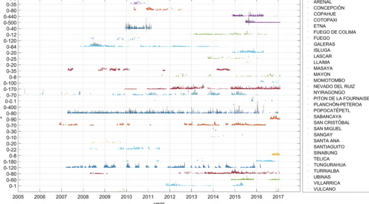
These are derived from minute-scale scan measurements, but we regard the daily emission as more representative of volcanic degassing because the sub-daily values may be subject to large variability introduced by meteorological effects, tidal influences, and other reasons (e.g. Bredemeyer and Hansteen, 2014; Dinger et al., 2018). We report the daily average SO2emission rate, standard deviation, different quantiles, and number of measurements in each day, as well as similar statistics for plume location, velocity, and cloud cover. Figure 3 shows the time series of daily SO₂flux between 1 March 2005 and 31 January 2017 for 32 volcanoes in NOVAC which produced a reasonable amount of valid data.

Figure 4 shows the mean emission and 25 %–75 % quantiles calculated from measured fluxes for all volcanoes during the same period. Results in numerical format are presented in Supplement S2. An important exception in this compilation

(8)

Figure 2.Schematics of the algorithm used to derive time-averaged emission of volcanoes in the NOVAC database.(a)Scattered sunlight spectra (shown in the figure as uncalibrated spectral radiance in arbitrary units; AUs) are checked for quality and combined to correct instrumental effects and to derive the differential slant column density (SCD) of SO₂through the non-linear DOAS method.(b)A collection of column densities in the scan is used to determine the baseline column density and the angular position of the centre of mass of the plume, to convert the slant to the vertical column density (VCD), and to estimate the completeness of the scanned plume.(c)Pairs of scans taken close in time by different instruments are used to derive plume altitude and direction. This is combined with plume speed using a meteorological model to derive the flux, including uncertainty. Individual flux measurements are chosen considering uncertainty, completeness, and other criteria.(d)If at least five valid measurements exist on a given day, statistics of daily emission are computed and reported in the NOVAC database. The background colour of the boxes indicates processing at the spectral level (white), scan level (grey), flux level (green), and external parameters (blue).

is Bárðarbunga volcano in Iceland; its Holuhraun eruption in 2014–2015 was monitored in detail, but the analysis of its data required special handling not apt for the procedure described here due to extreme measurement conditions and enormous amounts of gas (Pfeffer et al., 2018).

3.2 Long-term emission budgets and comparison with satellite-based data

The analysis of long-term data from automatic instrumental networks of this type presents a challenge for the extrapo- lation of (often irregular) sets of measurements in producing an estimation of time-averaged emissions. This challenge has to do with distinguishing periods of null observations, in the sense described above (i.e. when less than five measurements of good quality were obtained within a day), or those which are caused by instrumental (e.g. when no measurements were acquired) or observational (e.g. winds drifting the plume be- yond zone of observation) causes, from periods of legitimate low emission (i.e. absence of a plume). To account for these periods, we need additional information about the level of ac-

tivity, visual observations, photographic records, etc., which is not always available.

To deal with this problem, we have adopted the following strategy: if there are no statistics of emission for a given day and there were either no scanning measurements conducted or the mean plume direction (obtained from the meteorological model) lies outside the 5 %–95 % range of historical plume directions observed by the instruments, then no infer- ence can be made about the actual emission on that day, and the value is simply interpolated linearly between the near- est data points with valid observations. On the other hand, if measurements were done and the modelled wind data indicate that the plume should have been observed by the instrumental network, we attribute the lack of data for that day to low volcanic emission. The actual value of this low emission is chosen as the 5 % quantile of valid historical observations.

This value is chosen arbitrarily to represent an effective detection limit, noticing that the flux depends not only on the actual gas column density detection limit but also on the size and speed of the plume.

By filling in data in this way we can obtain a more reg- ular and accurate representation of the actual emission for

(9)

Figure 3.Time series of SO₂flux for 32 volcanoes in NOVAC from 1 March 2005 to 31 January 2017. Each dot (using a different colour for each volcano) represents the mean of all valid flux measurements obtained in the same day. The grey bars behind the dots represent the 25 %–75 % range of variability in flux for each day. The time series are presented as stacked plots with different scales for the flux, indicated as a range, to better represent the large range of variation between different volcanoes.

prolonged periods of time and calculate the corresponding statistics. The results of this procedure are shown in Fig. 5a–

c, where we present only the time series for volcanoes which have corresponding observations by OMI in the same period (12 out of 32) as reported by Carn et al. (2017). Notice also the time series of “only observed” data along with the corresponding time series of emission from the OMI sensor. Re- sults in numerical form are presented in Supplement S1.

3.3 NOVAC emission data repository

The results presented here are made public through a data repository hosted on the website https://novac.chalmers.se/

(last access: 1 October 2020). The site shows a map with the location of the volcanoes for which valid data have been produced. The dataset produced according to the methodology described here is labelled Version 1, and updates (temporal increments) and upgrades (different versions of data produced with improved methodology) are planned in the future. The dataset shows a summary of available raw data (i.e.

scans) collected by the instruments, along with a summary of valid fluxes derived from those measurements.

After selection of a volcano, a dedicated window presents a map with the setup of monitoring instruments, including coordinates and measurement parameters, a link to generic information about the volcano hosted on the Smithsonian

Institution’s Global Volcanism Program website (https://

volcano.si.edu/, last access: 1 October 2020), information on the responsible observatory and contact details, and the time series of daily mean SO2 emissions with associated statistics. The plots are easy to explore through different scaling and textual information. From each volcano page, data can be downloaded, after registering basic contact information and accepting the data use agreement, which states (e.g. for the case of Popocatépetl volcano) the following:

Large efforts have been made by the volcano observatories and institutions responsible for data collection and evaluation. Thus, data presented here can be used on the condition that these organiza- tions and people are given proper credit for their work, following normal practice in scientific communication:

(1) If data from this repository contributes an important part of the work, co-authorship should be offered to the listed contributors and the data-set should be cited.

(2) If data from this repository contributes only a small, but still important part of the work, the data-set should be cited.

To cite this data-set include this information:

(10)

Figure 4.Statistics of daily SO₂emission from 32 volcanoes in NOVAC from 1 March 2005 to 31 January 2017, for periods of time when data were being collected and yielding flux values above the detection limit. Blue markers show the average of all measured fluxes for each volcano during this period, and the error bars show the corresponding 25 % and 75 % quantiles.

****************************************

Delgado, H., Arellano, S., Rivera, C., Fickel, M., Álvarez, J., Galle, B., SO2 flux of - POPOCATEPETL- volcano, from the NO- VAC data-base; 2020; [Data set]; v.001;

doi:10.17196/novac.popocatepetl.001

****************************************

Additional data, data with higher time resolution and raw data may be made available upon request to the respective contacts, listed below.

This data-set has license: CC-BY 4.0

Notice that each dataset is assigned a registered and permanent digital object identifier (DOI).

The data files were prepared following the guidelines of the Generic Earth Observation Metadata Standard (GEOMS) (Retscher et al., 2011), which are generic metadata guidelines on atmospheric and oceanographic datasets adopted

for global initiatives, such as the Network for Detection of Atmospheric Composition Change (NDACC). The GEOMS standard requires a file format such as netCDF. This data format can be explored using openly available tools such as Panoply (https://www.giss.nasa.gov/tools/panoply/, last access: 1 October 2020). For users not familiarized with the netCDF format, a text format file, easily accessible through standard workbook or text editor applications and containing the same information that the netCDF file, is also available.

An example of such a file is presented in Supplement S3, and a list of all files is listed in Supplement S1.

The GEOMS standard requires data and metadata to be included in the same file. In the case of NOVAC, the metadata, required for the description and interpretation of the data, include the following:

– general information about the dataset

– data use agreement

(11)

Figure 5.

– data set description (site, measurement quantities, processing period, processing level, data version, DOI, ac- companying file, and date of file production)

– contact information – reference articles

– instrument(s) description (instrument type, spectrometer specification, fore-optics specifications, control unit specifications, instrument ID(s), site name(s), site coordinates, site measurement parameters, and instrument serial numbers)

– measurement description

– algorithm description (slant column densities, vertical column densities, SO₂flux and plume parameters, and statistics)

– expected uncertainty of measurement – description of appended results.

The data include the following:

– date according to universal time (UT)

– daily mean, standard deviation, quartiles, and number of valid SO₂flux measurements

– daily mean and standard deviation of plume speed – daily mean and standard deviation of plume direction – daily mean and standard deviation of plume height – daily mean and standard deviation of plume distance to

instruments and width

– daily mean and standard deviation of cloud cover (from re-analysis meteorological model).

Additional pages in the data repository provide details about the database, the data use agreement, technical details of the instrument, description of algorithms used for available data versions, contact information, and acknowledgements.

(12)

Figure 5.

The NOVAC data repository will be linked to other the- matic databases such as the Database of Volcanic Unrest (WOVOdat) of the World Organization of Volcano Obser- vatories, the database of the Global Volcanism Program of the Smithsonian Institution, the EarthChem data repository, the Global Emission InitiAtive (GEIA), the database of the Emissions of atmospheric Compounds and Compilation of Ancillary Data (ECCAD), and the database of the EU Coper- nicus Atmospheric Monitoring Service (CAMS).

4 Discussion

4.1 Comparison of emission from different volcanoes Figures 3 and 4 summarize the statistical information about the time series of emission for 32 volcanoes in NOVAC during 2005–2017. The plots show the daily and annual means and 25 %–75 % quantiles of daily SO₂ emission to represent variability. We highlight three main characteristics from these results: (i) the relatively large range of variation of

emissions, spanning typically up to 3 orders of magnitude in variability, for the same volcano at different times (Fig. 3);

(ii) the skewed nature of the distributions, with a dominance of low emission values (i.e. more frequent low emission rate values and a few large emission values that account for a considerable fraction of the total emission); and (iii) the large difference between the characteristic emission of different volcanoes (Fig. 4).

With respect to the intra-variability (for a particular volcano), we consider this to be one of the most important find- ings of long-term monitoring. As mentioned in the Introduc- tion, the production of high-sampling-rate, long-term measurements is relatively recent. Most compilations of measurements in the past include campaign-based estimates of gas emissions, typically during periods of enhanced activity, when a plume was visible and during short periods of time.

The skewed, large-range distributions of emission seem to be a general feature of degassing volcanoes and merit more attention. Our analysis, using only measured, i.e. not “filled- in”, data, indicates that the ratio of the first quartile to the

(13)

Figure 5.Time series of annual SO₂emission from 12 volcanoes in NOVAC for which corresponding results from OMI are available for the period 2005–2016. Dots show the annual mean emission rate with size linearly proportional to the number of valid measurements used for the average. The bars indicate the 25 % and 75 % quantiles of the daily means for each year. The series shown in blue correspond to observed plumes, while in black is the emission adjusted for periods of low degassing, when no plumes were observed (see text for details).

The series in red is the mean annual emission rate obtained from OMI measurements, with the size proportional to the precision (reciprocal of uncertainty) of the estimation and bars showing±1 standard deviation as reported by Carn et al. (2017).(a)Data from Copahue, Etna, Galeras, and Isluga.(b)Data from Masaya, Mayon, Nevado del Ruiz, and Nyiragongo.(c)Data from Popocatépetl, Tungurahua, Ubinas, and Villarrica. For details of the data in numerical format see Supplement S2.

mean of daily SO₂ fluxes reaches 43±14 % (±1σ), which means that the distribution of daily emission is dominated by low values. An important implication of this finding is that the low-emission spectrum of the distribution, which has usually not been measured in the past, contributes a significant amount of the total emission and should therefore be better characterized. Another is that short-term measurements may be skewed and could therefore not be representative of the long-term emission of a volcano.

Regarding the inter-variability (among different volcanoes), the observation of a large variance between sources is not new. Indeed, it has been speculated and partially shown by several authors (e.g. Brantley and Koepenick, 1995; An-

dres and Kasgnoc, 1998; Mori et al., 2013; Carn et al., 2017) that the partition between sources of volcanic degassing, particularly quiescent degassing, seems to follow either a log- normal or a power-law distribution. These distributions may seem similar, but choosing one over the other results in significant differences in estimating the global volcanic flux.

The relative importance of low vs. high emitters is also different for log-normal or power-law distributions. Evidently, with 32 volcanoes, out of perhaps 90–150 degassing volcanoes, it is not possible to verify these speculations with certainty. In any case, our measurements provide bounds for the contribution of weak emission sources, which have escaped observation by satellites during the same period.

(14)

4.2 Ground-based vs. space-based observations The recent compilation of global volcanic degassing from satellite-based measurements of OMI (Carn et al., 2017) offers an excellent opportunity for comparison with the measurements obtained from the ground with NOVAC instruments. First, both methods have operated for about the same period (since 2005); second, both sets of measurements are analysed independently in a consistent manner; and, third, the two datasets are focused on passive degassing. The quantification of SO₂flux from OMI observations was achieved by stacking of wind-rotated images over the course of a year, discarding both pixels contaminated by clouds and pixels with elevated column densities resulting from explosive eruptions. The co-added annual image is then fitted to a Gaussian distribution, following Fioletov et al. (2016), and the goodness of this fit is expressed as an “uncertainty”, but the actual uncertainty in the reported emission is not quantified but assumed in the order of 50 % (Fioletov et al., 2016;

Carn et al., 2017).

As mentioned above, it is necessary to fill in the measured SO₂emissions at each volcano during times when degassing was not detected but the instruments would have picked it up had it been occurring. The original, “un-filled” time series and the time series “filled” with low emission values are presented in Fig. 5a–c, along with the corresponding time series for OMI.

This comparison shows a general agreement in the temporal trends of annual emission for ground- and space-based methods but with differences in magnitude, which in some cases are considerable. Only 12 out of 32 volcanoes from NOVAC have corresponding detections from OMI. This is not surprising, as all volcanoes not observed by OMI are weak sources of emission, confined to the lower atmosphere and in some cases located in areas of persistent cloud cover.

Consequently, our dataset provides new data for several volcanoes, such as Sangay, Cotopaxi, Planchón-Peteroa, and Sinabung, and the largest dataset for all other volcanoes ever published.

Figure 5a–c, as well as Supplement S1, also show that the difference between ground- and space-based observations is reduced by the method of filling in low emission values in the patchy time series in NOVAC. Notwithstanding this better convergence, the differences are, in general, biased towards higher emission observed from satellites. There are many possible reasons for this; for example, the selection of data for OMI may tend to pick images from higher plumes that reach altitudes above low-level clouds, which may be the result of more explosive activity. Another reason could be that the data selection for NOVAC favours plumes with clear boundaries, and in some instances, high-gas-content plumes may be too wide and thus completely overcast the instruments, and, as a consequence, these are filtered out by the strict quality control filters applied to the dataset during our analysis.

However, the larger differences are caused by obvious reasons: for example, in the case of two nearby volcanoes, such as Nyiragongo–Nyamuragira (with a footprint of 13×24 km²), OMI cannot separate completely the contributions of each source, so they are reported as a complex.

In this respect, NOVAC can aid in discriminating between these sources, since the stations are deployed with a focus on Nyiragongo and the finer time resolution allows disentan- gling contributions, especially during periods of heightened activity at any of them. Other reasons for discrepancy are to be found in the different periods covered by the instruments, i.e. only daytime measurements for NOVAC, whereas OMI could in principle detect the emission occurring while overpassing at 13:30 LT in addition to remaining gas that was emitted emissions during the previous hours, potentially even during night. Other factors are the relatively large measurement uncertainties of both methods and different radiative transfer effects depending on altitude of surrounding plumes. A more in-depth study of these discrepancies is highly needed.

Finally, the method proposed here to account for days with null observations improves considerably the comparison with OMI in general. This is more obvious for volcanoes with constant emissions and good instrumental coverage, resulting in more valid measurements (represented by the size of the circles in Fig. 5a–c), which give us confidence in the validity of this approach.

4.3 The NOVAC inventory and past compilations of emission

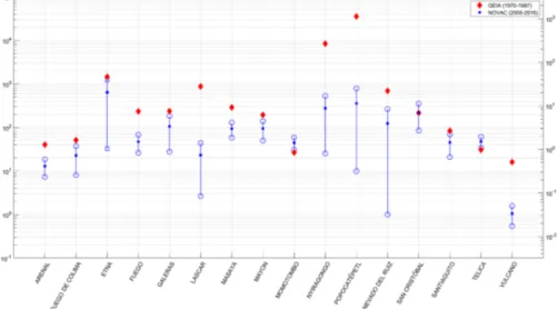
It is interesting to compare the emission statistics obtained from the NOVAC data with past compilations of emissions presented in other studies. We refer in particular to Andres and Kasgnoc (1998), who report the volcanic input during 1970–1997 to the Global Emission Inventory Activity (GEIA) database.

The results of a one-to-one comparison between the emissions reported for quiescent degassing volcanoes in GEIA and NOVAC are presented in Fig. 6. There are a few volcanoes reported in GEIA which are not part of NOVAC yet;

conversely, some volcanoes were monitored in NOVAC that were not active and thus not considered during the period reported in GEIA. A comparison can only be done for the 16 volcanoes present in both datasets. Undoubtedly, the reported values are not expected to coincide, considering that the measurements were not obtained during the same periods, and, as revealed by the NOVAC results, volcanic gas emission is by no means a stationary process over time. How- ever, it is important to highlight that the recent measurements from NOVAC provide a characteristic range of variation for the volcanic sources, which in most cases, but not all, accom- modate the results of past, punctuated observations. But we notice also that, except for Momotombo, San Cristóbal, and Telica, the mean emissions reported in GEIA lie on the up-

(15)

Table1.StatisticsofmeasuredSO2fluxduring2005–2016for32volcanoesinNOVAC(NetworkforObservationofVolcanicandAtmosphericChange).Thereportedvaluesarethe arithmeticmean(average)ofthedifferentdailystatistics(mean;standarddeviation,SD;andquartiles)includedintheNOVACdatafiles.DOI:digitalobjectidentifier. VolcanoStatisticsofmeasuredSO2NumberofdayswithReferenceDOIlink fluxduring2005–2016[kg/s]validfluxstatistics MeanSDFirstMedianThirdwithrespecttodays quartilequartilewithmeasurements Arenal1.590.801.041.431.9838/350Avardetal.(2020a)https://doi.org/10.17196/novac.arenal.001 Concepción6.102.014.665.927.30186/795Saballosetal.(2020a)https://doi.org/10.17196/novac.concepcion.001 Copahue9.023.616.518.3711.03288/476Velásquezetal.(2020a)https://doi.org/10.17196/novac.copahue.001 Cotopaxi8.945.315.248.3811.76447/2829Hidalgoetal.(2020a)https://doi.org/10.17196/novac.cotopaxi.001 Etna40.7212.1831.9838.8847.94192/875Salernoetal.(2020)https://doi.org/10.17196/novac.etna.001 FuegodeColima2.721.661.542.413.60185/2750Delgadoetal.(2020a)https://doi.org/10.17196/novac.fuegodecolima.001 Fuego3.531.302.613.414.2430/407Chignaetal.(2020a)https://doi.org/10.17196/novac.fuegoguatemala.001 Galeras8.993.806.358.4611.11704/3340Chacónetal.(2020a)https://doi.org/10.17196/novac.galeras.001 Isluga8.113.655.467.3510.18230/497Bucareyetal.(2020a)https://doi.org/10.17196/novac.isluga.001 Lascar2.621.431.612.323.3775/919Bucareyetal.(2020b)https://doi.org/10.17196/novac.lascar.001 Llaima10.083.427.6610.0812.494/1308Bucareyetal.(2020c)https://doi.org/10.17196/novac.llaima.001 Masaya3.871.382.913.744.70500/772Saballosetal.(2020b)https://doi.org/10.17196/novac.masaya.001 Mayon7.012.505.306.598.29102/1173Bornasetal.(2020)https://doi.org/10.17196/novac.mayon.001 Momotombo1.850.601.451.752.1835/158Saballosetal.(2020c)https://doi.org/10.17196/novac.momotombo.001 NevadodelRuiz7.764.964.236.9110.431281/2431Chacónetal.(2020b)https://doi.org/10.17196/novac.nevadodelruiz.001 Nyiragongo19.148.8912.7117.7124.52432/1758Yalireetal.(2020)https://doi.org/10.17196/novac.nyiragongo.001 PitondelaFournaise9.586.774.658.6213.2022/3402DiMuroetal.(2020)https://doi.org/10.17196/novac.pitondelafournaise.001 Planchón-Peteroa0.050.020.030.040.064/22Velásquezetal.(2020b)https://doi.org/10.17196/novac.planchonpeteroa.001 Popocatépetl24.4812.2815.8123.2731.961207/3306Delgadoetal.(2020b)https://doi.org/10.17196/novac.popocatepetl.001 Sabancaya11.865.857.5610.7615.10126/162Masiasetal.(2020b)https://doi.org/10.17196/novac.sabancaya.001 SanCristóbal8.873.416.448.3410.861028/1557Saballosetal.(2020d)https://doi.org/10.17196/novac.sancristobal.001 SanMiguel22.516.1719.4222.2525.254/160Montalvoetal.(2020a)https://doi.org/10.17196/novac.sanmiguel.001 Sangay7.493.344.877.159.737/536Hidalgoetal.(2020c)https://doi.org/10.17196/novac.sangay.001 SantaAna1.960.561.551.862.3622/868Montalvoetal.(2020b)https://doi.org/10.17196/novac.santaana.001 Santiaguito3.221.801.962.834.08170/570Chignaetal.(2020b)https://doi.org/10.17196/novac.santiaguito.001 Sinabung4.422.073.053.955.14108/173Kasbanietal.(2020)https://doi.org/10.17196/novac.sinabung.001 Telica0.830.310.600.781.00205/460Saballosetal.(2020e)https://doi.org/10.17196/novac.telica.001 Tungurahua17.127.9311.5416.1721.811100/3463Hidalgoetal.(2020b)https://doi.org/10.17196/novac.tungurahua.001 Turrialba11.504.987.9810.9614.48614/1878Avardetal.(2020b)https://doi.org/10.17196/novac.turrialba.001 Ubinas3.522.002.093.204.62375/622Masiasetal.(2020a)https://doi.org/10.17196/novac.ubinas.001 Villarrica6.752.584.906.288.23203/2001Velásquezetal.(2020c)https://doi.org/10.17196/novac.villarrica.001 Vulcano0.200.060.150.190.2434/1180Vitaetal.(2020)https://doi.org/10.17196/novac.vulcano.001

(16)

Figure 6.Comparison of emission statistics for 16 volcanoes of the NOVAC and GEIA datasets. For NOVAC the simple averages of the annual mean (filled blue dots) and±1 standard deviations (un-filled blue dots) for the years 2005–2016 are depicted. The values for GEIA are obtained from Andres and Kasgnoc (1998) for passively degassing and sporadically degassing volcanoes only.

per end or higher than those reported here. We speculate that such systematic difference may be due to biased sampling during periods of high emission that was the basis for most of the Andres and Kasgnoc (1998) compilation. Long-term observation also captures periods of quiescence that may be the reason for lower values.

5 Code availability

The NOVAC Post Processing Program and other software used in NOVAC are open-source projects available at https://doi.org/10.5281/zenodo.4615189 (Johansson, 2021).

6 Data availability

More information about NOVAC can be found at the website https://novac-community.org/ (last access: 1 October 2020).

Raw data from NOVAC are accessible by request to the local observatory responsible for the measurements. The dataset obtained for this study can be accessed, free of charge, through a dedicated website (https://novac.chalmers.se/, last access: 1 October 2020). The datasets of individual volcanoes can be accessed through the DOI links provided in Ta- ble 1. Updates of the time series, addition of new volcanoes, and release of data versions resulting from improved analysis are planned.

7 Conclusions and outlook

In this study, we report the results of post-processing of SO₂ mass emission rate measurements at 32 volcanoes of the NO- VAC network during 2005–2017. This is, to our knowledge, the densest (∼10–50 measurements per volcano per day for

up to 12 years, 32 volcanoes) database of volcanic degassing obtained by a standardized method. Since the ScanDOAS method is subject to multiple and potentially large sources of uncertainty, considerable attention has been given to the selection of high-quality measurements on which to base the reported statistics.

Independent studies (e.g. Stoiber et al., 1987; Krueger et al., 1995; Halmer et al., 2002; Andres and Kasgnoc, 1998;

Carn et al., 2017) have demonstrated over the years that passive degassing dominates, in time and magnitude, the time-averaged global volcanic emission. At the same time, this component of volcanic emission can produce a persistent impact on local, regional, or global scales and potentially affect the climate system. Observational limitations have hindered quantifying the magnitude and variability of global volcanic degassing in the past at the level of detail obtained by a global ground-based network like NOVAC.

This database will therefore represent an important contribution to global emission inventories, which are typically based on sporadic and short-term investigations of emission during periods of heightened activity. Moreover, the results from measurements in NOVAC complement the observations from satellite platforms, which on an operational basis during the past decade were more suited for quantification of explosive degassing.

The measurements performed in NOVAC provide more information than the gas emission rate of SO2. First, spectroscopic analysis of the data can be used for retrieving the abundances of other species, as has been proven most sys- tematically for the case of BrO (Lübcke et al., 2014; Dinger et al., 2018; Warnach et al., 2019). Second, in principle all the variables involved in the calculation of the mass flow rate can be obtained from the measurements (plume location, dimen-