1.2 Genetic association studies

METHODS TO INVESTIGATE GENE-STRATA INTERACTION IN GENOME-WIDE ASSOCIATION META-ANALYSES ON THE EXAMPLE OF OBESITY

Dissertation

zur Erlangung des Doktorgrades der Biomedizinischen Wissenschaften

(Dr. rer. physiol.)

der

Fakultät für Medizin der Universität Regensburg

vorgelegt von Thomas Winkler

aus Regensburg

im Jahr 2015

Dekan: Prof. Dr. Dr. Torsten E. Reichert Betreuer: Prof. Dr. Iris Heid

TABLE OF CONTENTS

1 Introduction ... 5

1.1Obesity and genetics of obesity ... 5

1.2Genetic association studies ... 7

1.3Statistical models and methods for genetic association studies ... 10

1.3.1 The linear regression model ... 10

1.3.2 SNP genotype models ... 11

1.3.3 SNP association testing ... 11

1.3.4 Genome-wide association studies ... 12

1.3.5 Genome-wide association meta-analyses ... 12

1.4Genome-wide association meta-analyses for obesity traits: The GIANT consortium ... 12

1.5Gene-strata interaction effects in genetic association studies ... 14

1.5.1 Modelling gene-strata interaction effects in large-scale GWAMAs ... 14

1.5.2 Methods to account for and to identify gene-strata interaction effects ... 16

1.6Objectives ... 16

2 Stratified GWAMA approaches to screen for difference between two strata ...19

2.1Materials and Methods ... 20

2.1.1 Assumptions and definitions ... 20

2.1.2 Testing for stratum-difference ... 21

2.1.3 Statistical tests to filter stratified GWAMA data sets prior to difference testing ... 21

2.1.4 A systematic scheme of stratified GWAMA approaches to identify stratum-difference ... 22

2.1.5 Simulation-based evaluation of type 1 error ... 25

2.1.6 Analytical computation of power ... 26

2.2Results... 31

2.2.1 Simulation-based evaluation of type 1 error ... 31

2.2.2 Analytical power comparison ... 34

3 Stratified GWAMA approaches to screen for G x AGE x SEX interaction effects ...51

3.1Materials and Methods ... 52

3.1.1 Assumptions and definitions ... 52

3.1.2 Testing for G x AGE x SEX interaction given the age- and sex-stratified GWAMA model ... 53

3.1.3 Statistical tests to filter stratified GWAMA data sets prior to G x AGE x SEX interaction testing ... 54

3.1.4 A systematic scheme of age- and sex-stratified GWAMA approaches to identify G x AGE x SEX interaction ... 56

3.1.5 Simulation based evaluation of type 1 error ... 58

3.1.6 Analytical computation of power ... 59

3.2Results... 65

3.2.1 Simulation-based evaluation of type 1 error ... 65

3.2.2 Analytical power comparison ... 68

4 Application to stratified GWAMAs for obesity traits ...74

4.1Materials and Methods ... 74

4.1.3 Utilizing the GIANT SMOKING data for WHRadjBMI to screen for stratum-difference

under an unbalanced design ... 76

4.1.4 Utilizing the GIANT AGE x SEX data for WHRadjBMI to screen for G x AGE x SEX interaction ... 77

4.2Results... 77

4.2.1 Identification of sex-differences in genetic effects for WHRadjBMI... 77

4.2.2 Identification of differences between smokers and non-smokers in genetic effects for WHRadjBMI ... 84

4.2.3 Identification of G x AGE x SEX interaction for WHRadjBMI ... 85

5 The Easy R packages ...87

5.1The Easy framework ... 88

5.1.1 Object oriented programming ... 88

5.1.2 Big data ... 89

5.1.3 Requirements and performance ... 89

5.2EasyQC ... 90

5.3EasyStrata ... 92

5.3.1 Statistical Functionality ... 92

5.3.2 Graphical Functionality ... 94

6 Discussion ...96

6.1Summary of main results... 96

6.1.1 Optimal stratified GWAMA approaches to screen for stratum-difference ... 96

6.1.2 Optimal stratified GWAMA approaches to screen for G x AGE x SEX interaction ... 97

6.1.3 Application to stratified GWAMAs for obesity traits ... 98

6.1.4 Software for conduct and evaluation of stratified GWAMAs ... 99

6.2Stratified GWAMA methods to tackle gene-environment interaction effects ... 99

6.2.1 Reported methods to account for G x E interaction effects ... 99

6.2.2 Reported methods to detect G x E interaction effects ... 101

6.2.3 Relating stratified modelling to interaction modelling ... 102

6.3Stratum-specific effects in the genetics of obesity ... 104

6.3.1 Sex-differences in genetic effects for body fat distribution ... 104

6.3.2 Differences in genetic effects for obesity measures between smokers and non- smokers ... 110

6.3.3 Age- and sex-specific genetic effects for obesity measures ... 110

6.4Relevance of the developed Easy software packages ... 111

6.5Strengths and Limitations ... 114

6.6Conclusion and Outlook ... 115

7 Summary ... 118

8 Zusammenfassung ... 120

9 Appendix ... 122

9.1Validation of simulated data sets used for evaluation of type 1 error of approaches involving two strata ... 122

9.1.1 Validation of simulated data sets for 1-stage approaches ... 122

9.1.2 Validation of simulated data sets for 2-stage approaches ... 123

9.2Simulation-based inference of statistical dependence between filtering and difference

tests ... 124

9.3Simulation-based estimation of power for approaches with dependent discovery steps ... 125

9.3.1 Estimation of discovery power for approach [𝑺𝒕𝒓𝒂𝒕𝜶𝟏, 𝑫𝒊𝒇𝒇𝜶𝟐] → [𝑫𝒊𝒇𝒇𝜶𝒃𝒐𝒏𝒇] ... 125

9.3.2 Estimation of discovery power for approach [𝑱𝒐𝒊𝒏𝒕𝜶𝟏, 𝑫𝒊𝒇𝒇𝜶𝟐] → [𝑫𝒊𝒇𝒇𝜶𝒃𝒐𝒏𝒇] ... 126

9.4Validation of simulated data sets used for evaluation of type 1 error of age- and sex- stratified GWAMA approaches ... 127

9.5Simulation-based inference of statistical dependence between steps for the age- and sex- stratified GWAMA approaches ... 128

9.5.1 Dependence between filtering and difference-of-difference tests ... 128

9.5.2 Dependence between marginal age- and marginal sex-tests ... 129

9.6Simulation-based estimation of power for age- and sex-stratified GWAMA approaches that involve dependent statistical tests ... 130

9.6.1 Estimation of filtering power for approach [𝑴𝒂𝒓𝑺𝒕𝒓𝒂𝒕𝜶𝟏 → 𝑫𝒊𝒇𝒇𝑫𝒊𝒇𝒇𝜶𝒃𝒐𝒏𝒇] ... 130

9.6.2 Estimation of filtering power for approach [𝑴𝒂𝒓𝑱𝒐𝒊𝒏𝒕𝜶𝟏 → 𝑫𝒊𝒇𝒇𝑫𝒊𝒇𝒇𝜶𝒃𝒐𝒏𝒇] ... 131

9.7Example EasyStrata pipeline to evaluate sex-difference ... 132

9.8Extended features and applicability of EasyStrata ... 134

9.8.1 Extended applicability ... 134

9.8.2 Extended statistical methods ... 135

9.8.3 Extended graphical features ... 136

References ... 140

List of abbreviations ... 147

List of publications... 148

Related publications and description of own contribution ... 148

Other publications ... 149

Selbstständigkeitserklärung ... 152

Acknowledgements ... 153

Curriculum Vitae ... 154

1 Introduction

The overarching goal of epidemiology is to study the etiology of diseases. Diseases with substantial genetic components are called heritable diseases and are clustered into monogenic and complex diseases.

Monogenic diseases are typically rare and caused by mutations in a single gene.

Examples for monogenic diseases are Cystic Fibrosis, Huntington's disease, Sickle cell anemia or the fragile X syndrome.

In contrast, complex diseases are characterized by a complicated interplay of multiple genetic and environmental factors. They are also referred to as multifactorial diseases.

Examples for complex diseases are common diseases such as cancer, diabetes, cardiovascular disease, asthma, psychiatric illnesses, inflammatory diseases or obesity.

Single genetic factors typically contribute very little to the development of complex diseases.

However, an accumulation of multiple small but disadvantageous genetic factors in combination with environmental factors that may further be interacting with each other contributes substantially to the development of complex diseases.

Genetic epidemiology is the scientific field that aims to unravel the complicated interplay of genetic and environmental factors that influence complex disease development (Khoury, Beaty, & Cohen, 1993). Revealing the underlying genetic mechanism is pivotal for understanding disease etiology and may lead to novel therapies, improved prediction or targeted prevention programs.

1.1 Obesity and genetics of obesity

Over the past decades, obesity has become one of the world’s major healthcare problems (Caballero, 2005). In particular the westernized countries have developed highly obesogenic environments that have led to a sharp increase in obesity prevalence: In Germany, more than 37% of individuals are estimated to be overweight (body mass index, BMI ≥ 25 kg/m² and BMI < 30 kg/m²) and another 20% are estimated to be obese (BMI ≥ 30 kg/m²) (Rubner- Institut, 2008). Obesity is strongly associated with mortality, an association that is mediated through increased risk for different morbidities, such as cardiovascular diseases (e.g., coronary heart disease), metabolic diseases (e.g., type 2 diabetes), psychiatric diseases (e.g., depression), or cancer (Haslam & James, 2005; Samanic, Chow, Gridley, Jarvholm, &

Fraumeni, 2006). Due to its severe consequences, obesity has overcome the impact of smoking and drinking on individual health and on total healthcare costs (Moriarty et al., 2012;

Obesity can generally be classified into two categories that are independently associated with increased risk for morbidity and mortality (Pischon et al., 2008): Overall obesity as measured by BMI reflects total body mass and central obesity as measured by waist circumference or waist-hip ratio (WHR) reflects abdominal obesity or body fat distribution.

Obesity risk as well as BMI and WHR are known to be influenced by environmental factors, such as sex, age, smoking, nutritional factors and physical activity. For example, the obesity prevalence is generally higher in women than in men (Lovejoy, Sainsbury, & Stock Conference Working, 2009). Considering life course, men slowly accumulate fat around the waist, whereas women store more fat around hips at younger ages and begin to accumulate more fat around the waist after menopause, when estrogen levels drop (Kirchengast, 2010;

Loomba-Albrecht & Styne, 2009). Furthermore, moderate smokers display lower body weight, lower BMI, but higher waist circumference than non-smokers and gain weight after smoking cessation (Chiolero, Faeh, Paccaud, & Cornuz, 2008). Notably, heavy smokers display increased weight and BMI, which may be due to an accumulation of risky behaviors, such as low physical activity or high caloric intake that overcomes the BMI decreasing effect of moderate smoking on obesity measures. Finally, a reasonable diet and increased physical activity lowers the risk of obesity and related diseases (Lakka & Bouchard, 2005), but both is incredibly difficult to implement into obese persons’ life styles.

Both, overall and central obesity, involve substantial genetic components comprising high estimates of heritability (i.e., phenotypic variance explained by genetics, typically >70%

for BMI, and >45% for WHR) (Farooqi & O'Rahilly, 2000; Rose, Newman, Mayer-Davis, &

Selby, 1998; Zaitlen et al., 2013).

Although obesity can generally be classified as a common complex disease, there are also some rare monogenic forms of obesity.

The prominent melanocortin-4 receptor (MC4R) gene has multiple implications in obesity. Generally, MC4R acts in the central melanocortinergic system and regulates food and energy intake (Adan et al., 2006). On the one hand, a single rare mutation in MC4R gene was shown to cause a specific monogenic form of childhood obesity (Farooqi et al., 2003). On the other hand, a common variant located near the MC4R gene (present in ~24%

of the general population) was shown to be associated with increased BMI (Loos et al., 2008). Although the single common MC4R variation explained only ~0.10% of the total BMI variation, it helped highlighting an interesting biological pathway: The common risk variant showed decreased MC4R protein levels in the hypothalamus that leads to increased appetite and decreased satiety (Qi, Kraft, Hunter, & Hu, 2008). Therefore, MC4R agonists are interesting candidates for the pharmacological development of drugs to treat not only rare monogenic forms but also the common form of obesity (Adan et al., 2006).

Another prominent obesity gene that illustrates the complex interplay of genetic and environmental factors is the ‘fat mass and obesity associated’ (FTO) gene. Initially identified for its association with type 2 diabetes (T2D), follow-up analyses adjusted the T2D association for BMI and showed that the T2D association of the common FTO variant disappeared (Frayling et al., 2007). This suggested that the impact of the common risk variant in FTO (present in ~42% of the general population) on T2D was mediated through obesity. Functional follow-up studies using gene knock-out mice revealed that FTO variants were implicated in energy homeostasis (Fischer et al., 2009). This was one of the first successful attempts to translate genetic epidemiology association study results into functional processes and consequences affecting body weight regulation. Finally, one of the first gene-environment interactions highlighted for obesity was observed for FTO: The effect of FTO variants on obesity risk was shown to be attenuated by higher physical activity levels (Andreasen et al., 2008).

Besides physical activity, other environmental factors such as sex, age, smoking or nutrition may modify genetic effects on obesity and may – at least in part – explain known differences in obesity measures between men and women, between smokers and non- smokers, between individuals on high-calorie and low-calorie diet or explain the changes in body shape over life course.

In summary, these examples illustrate the importance to investigate the genetic underpinning of obesity to further the understanding of involved mechanism that may ultimately lead to improved therapeutic options.

1.2 Genetic association studies

The aim of genetic association studies is to identify association between genetic variation and an outcome of interest, such as disease (e.g., type 2 diabetes) or disease-relevant parameters (e.g., BMI). The outcome is referred to as phenotype in the following.

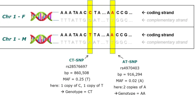
The most frequent forms of genetic variation in the Deoxyribonucleic Acid (DNA) are single nucleotide polymorphisms (SNPs). Each SNP denotes a single base-exchange that originated at some point during evolution and is located at a specific position in the DNA sequence (Figure 1). Most SNPs are bi-allelic comprising two possible nucleotide variations, also referred to as alleles. The combination of two alleles - one on the maternal and one on the paternal chromosome - makes up the so-called genotype of the SNP for a specific person. SNPs are called common if the less frequent allele (i.e., minor allele) is present in at least 5% of individuals in a population. Less frequent SNPs are called rare. More than 60 million SNPs are known to date including approximately 10 million SNPs with minor allele frequency (MAF) greater than 1% (Sherry et al., 2001).

Figure 1. Schematic presentation of two SNPs. Shown are the coding and the complementary strand for both versions of chromosome 1 (paternal and maternal chromosome 1).

In the early 2000s, SNP-phenotype associations have mainly been identified through hypothesis-driven candidate-gene approaches. Such approaches require a-priori knowledge on the biology of the phenotype and on the possible implications of potential candidate genes. The problem with this approach was that it required choosing the right candidate gene in advance, a process that can be difficult because the decision has to be made on the current state of knowledge, which may be limited. Overall, candidate-gene approaches were often unsuccessful, mostly because wrong candidates were chosen or because the power of single candidate-gene studies was too low.

Instead, genome-wide association studies (GWAS) have recently been found to be more efficient. GWAS are hypothesis-free approaches that simultaneously screen a dense field of millions of SNPs - spread across the whole genome - for association. Importantly, to avoid large numbers of false positive findings, GWAS require rigorous control for the multiple testing of millions of variants.

GWAS were only yet enabled through technical advances in genotyping since 2005 (Hirschhorn & Daly, 2005). Improved chip-based microarray technologies nowadays allow study centres to effectively assess one million or more SNPs for large studies including thousands of individuals. A large number of genotyping chips have been developed over the past years (Distefano & Taverna, 2011). Besides genome-wide chips that cover SNPs equally spread across the whole genome, customized genotyping chips were designed that fine-map particular regions of interest. For example, the MetaboChip specifically covers regions associated with metabolic disorders, including obesity (Voight et al., 2012).

Besides advances in direct genotyping chip technologies, genotype imputation has largely contributed to the success of GWAS (Y. Li, Willer, Sanna, & Abecasis, 2009).

Imputation methods allow for inferring unmeasured variants on the basis of reference sequence data. Imputation is pivotal for comparing association results across studies with different genotyping platforms. Over the past years, almost all GWAS have used imputed data with up to ~2.5M variants based on HapMap reference panels (International HapMap, 2005).

A challenge in GWAS is that genetic effects are typically small. For example, in obesity, the largest genetic effect observed for BMI (near FTO) explains only ~0.34% of the total BMI variation (Speliotes et al., 2010). Medium genetic effects on BMI are even smaller by ten-fold and explain only ~0.04% of the BMI variation. Given the multiple testing burdens, identification of such subtle effects necessitates large sample sizes and single GWAS involving ~1,000 individuals are often underpowered.

One way to increase power to detect small genetic effect sizes is to pool multiple GWAS in so-called genome-wide association meta-analyses (GWAMAs). Meta-analysis of aggregated statistics across multiple studies and for each SNP genome-wide allows for increasing power when an individual participant data analysis is not possible. This is typically the case in genetic studies because study partners are most often not allowed to share individual level participant genotype data due to ethical constraints. Over the past years, many GWAMA consortia have emerged and multiplied the total sample size for several diseases and disease-relevant parameters. For example, one of the largest GWAMA consortia worldwide is the Genetic Investigation of Anthropometric Traits (GIANT) consortium. GIANT has set out to investigate the genetic underpinning of anthropometric and obesity traits (primarily focusing on height, BMI and WHR) involving hundreds of single GWAS and hundreds of thousands of individuals altogether.

Taken together, GWAS and GWAMAs have successfully been employed over the past years and have led to a major increase in the number of known SNP-phenotype associations (Visscher, Brown, McCarthy, & Yang, 2012; Welter et al., 2014). So far, more than 14,000 SNP-phenotype associations have been reported that are accessible through publicly available data bases, such as the GWAS catalogue (Hindorff et al., 2009).

Yet, despite the large success of GWAS, a substantial fraction of the heritability still remains unexplained for most phenotypes (Manolio et al., 2009). A fraction of the missing heritability might be explained by rare variants (MAF < 5%, expected to yield larger effect sizes than common variants) or by structural variation (e.g., copy number variants such as insertions or deletions), both of which have mostly been missed due to low power or due to unsuitable array designs (genotyping arrays primarily focused on common variants, i.e.,

systematic screens that employ novel genotyping arrays as well as denser imputation reference panels.

Another fraction of the missing heritability might be explained by gene-environment interaction effects that have been missed and ignored by the commonly conducted genome- wide scans focussing on overall associations. Detecting gene-environment interaction effects requires systematic screens that employ large sample sizes, extended statistical methods and software tools that are applicable to large-scale genome-wide data sets. Yet, such methods are poorly understood and software tools are lacking.

1.3 Statistical models and methods for genetic association studies

The following chapter introduces statistical models and concepts of SNP-phenotype association testing, GWAS and GWAMAs.

1.3.1 The linear regression model

A general SNP-trait association test is based on regression methods that fit a Generalized Linear Model (GLM). A GLM allows for correcting for potential confounders by using additional covariables. For a continuous phenotype 𝑌, a linear regression model is considered:

𝑌 = ∝ +𝛽𝐺 + 𝛽_𝐶1𝐶₁+ ⋯ 𝛽_𝐶𝑘𝐶_𝑘+ 𝜀, 𝜀~𝑁(0, 𝜎²) (1).

Here, 𝐺 denotes the SNP genotype, 𝐶_𝑖 are the co-variables, 𝛼 is the intercept of the regression model, 𝛽 the genetic effect on 𝑌, and 𝜀 a random error variable, also called residual. The linear regression model is based on some important assumptions that involve (i) lack of auto-correlation (i.e., residuals are assumed to be independent and to follow a normal distribution with zero mean and residual variance 𝜎²), (ii) homoscedasticity (i.e., the residual variance is assumed to be constant across genotype), and (iii) a linear and additive relationship between genotypes and phenotypes. To ensure comparability of the phenotype across studies, one approach is to normalize (or to standard normalize) the phenotype per study which yields 𝑌~𝑁(𝜇_𝑌, 𝜎_𝑌²) (or 𝑌~𝑁(0,1)).

In genetic epidemiology, regression models are usually adjusted for other epidemiological factors (added as co-variables) that either have an impact on the phenotype or have an impact on both, the phenotype and the genotype.

Adjusting for factors that are known to influence the phenotype (only) reduces the phenotypic variance by the proportion that is explained through the respective co-variable and as such increases the power to find the genotype-phenotype association. For example,

due to their well-known influence on anthropometric traits, GIANT requests contributing study partners to adjust for sex and age.

Adjusting for factors that are known to influence both the phenotype and the genotype (i.e., confounders), prevents from observing an association between genotype and phenotype that is actually driven by the hidden confounding variable. Genetic association models are usually adjusted for potential confounding through population stratification that reflects systematic diversities between population substructures. To avoid such confounding, in many cases the first ten independent genotype dimensions (principle components) are added to the regression model as co-variables.

1.3.2 SNP genotype models

Usual genotype models are the recessive, the dominant and the additive model. Consider a SNP with two alleles: Major allele A denoting the more frequent allele, and minor allele a denoting the less frequent allele. For a specific SNP, an individual can take three possible genotype states: AA (two copies of the major allele), Aa (one copy of the major and one of the minor allele) and aa (two copies of the minor allele).

The dominant model implies that individuals with one or two copies of the minor allele exhibit the phenotype (with equal probability). Thus, the genotype variable is coded G = 0 for genotype AA and coded G = 1 for genotypes Aa and aa.

The recessive model implies that only individuals with two copies of the minor allele exhibit the phenotype. Thus, the genotype variable is coded G = 0 for genotypes Aa and AA, and coded G = 1 for genotype aa.

The commonly used additive model implies that the probability to exhibit the phenotype increases linearly with each additional copy of the minor allele. Thus, the genotype variable is coded G = 0 for genotype AA, G = 1 for genotype Aa and G = 2 for genotype aa. With MAF being the minor allele frequency of a particular SNP, the additively modelled SNP genotypes 0,1 and 2 occur with probabilities (1–MAF)², 2MAF(1–MAF) and MAF², respectively, if Hardy-Weinberg equilibrium is fulfilled (Edwards, 2008). For large sample sizes, the binomial genotype distribution approximates a normal distribution with genotypic mean 𝜇_𝐺 = 2 ∙ 𝑀𝐴𝐹 and genotypic variance 𝜎_𝐺² = 2𝑀𝐴𝐹(1 − 𝑀𝐴𝐹).

1.3.3 SNP association testing

To infer whether the modelled SNP genotype is associated with the phenotype, i.e., whether the genetic effect on Y - estimated from the regression model - is significantly different from zero, a t test can be conducted that compares the null hypothesis 𝐻₀: 𝛽 = 0versus the alternative hypothesis 𝐻_𝐴: 𝛽 ≠ 0. Herewith, a test statistic 𝑇 = 𝑏/𝑠𝑒(𝑏) is employed, where n

error ofb. Assuming the nulll hypothesis, the test statistic T follows a t distribution with n-2 degrees of freedom (df), i.e., 𝑇 ~ 𝑡(𝑛 − 2)|𝐻₀. The t test yields a SNP association P-Value P.

1.3.4 Genome-wide association studies

In GWAS, the association testing is conducted separately and simultaneously for the millions of SNPs available for a study. To avoid huge numbers of false positive findings, SNP-specific association results are corrected for the multiple testing. Typically in HapMap imputation based GWAS, a conservative genome-wide significance threshold of  = 5 x 10^-8 is applied that Bonferroni-corrects the usual 5% -level for an approximate number of one million (1M) independent SNP association tests (Johnson et al., 2010).

1.3.5 Genome-wide association meta-analyses

For each SNP, each GWA study j provides study-specific summary estimates such as the genetic effect estimate 𝑏^𝑗, the corresponding standard error 𝑠𝑒(𝑏^𝑗), the association P-Value 𝑃^𝑗 and the sample size 𝑛^𝑗. To obtain pooled genetic effect estimates and standard errors for each SNP, an inverse-variance weighted meta-analysis can be conducted, computing

𝑏 =∑_𝑗𝑏^𝑗/𝑠𝑒(𝑏^𝑗)²

∑ 1/_𝑗 𝑠𝑒(𝑏^𝑗)² and 𝑠𝑒(𝑏_{) = √} ¹

∑ 1/_𝑗 𝑠𝑒(𝑏^𝑗)²

(2).

In the meta-analytical setting, b and se(b) are referred to as pooled genetic effect estimate and pooled standard error. As in single study association testing, a t test statistic 𝑇 = 𝑏/𝑠𝑒(𝑏)~ 𝑡(𝑛 − 2)|𝐻₀ is utilized to infer, whether the pooled genetic effect is significantly different from zero. The t test yields a pooled overall association P-Value P. The meta- analysis formulae (2) assume a fixed effect model across studies. For homogeneous genetic effects across studies, the pooled genetic effect estimates and standard errors are approximately the same as the genetic effect estimates and standard errors obtained from a single regression model using one large study involving all individuals (Behrens, Winkler, Gorski, Leitzmann, & Heid, 2011).

1.4 Genome-wide association meta-analyses for obesity traits: The GIANT consortium

One of the largest GWAMA consortia worldwide is the Genetic Investigation of ANthropometrics Traits (GIANT) consortium (Figure 2). This consortium has set out to describe the genetic underpinning of anthropometric and obesity traits. For the obesity traits, the primary focus is on body mass index (BMI, as a measure of overall obesity) and on waist

hip ratio adjusted for BMI (WHRadjBMI, as a measure of central obesity that is independent of BMI).

Since 2006, GIANT has published multiple rounds of meta-analyses on these primary traits, with each round iteratively increasing the total sample size, increasing the total number of studies involved, adding novel genotyping chip technologies and incorporating larger imputation reference panels (Heid et al., 2010; Lindgren et al., 2009; Loos et al., 2008;

Speliotes et al., 2010; Willer et al., 2009). In 2010, the number of identified loci was raised to 32 for BMI (using discovery GWAS data from up to 123,865 individuals) and to 14 for WHR_adjBMI (using discovery GWAS data from up to 77,167 individuals).

Figure 2. GIANT consortium studies involved in the 2010 meta-analyses (for more information see the GIANT consortium website, www.broadinstitute.org/collaboration/giant).

Due to the known sex-differences in obesity measures, the identified loci were investigated for sex-differences in consecutive follow-up analyses (using men- and women- specific GWAS results that have been provided by the study partners). No significant sex- difference was observed in any of the 32 detected BMI loci. In contrast, seven of the 14 overall associated WHR_adjBMI loci were found to be sex-specific, and all of the seven displayed significantly stronger effects in women than in men (Heid et al., 2010).

overall association, an approach that might have missed other sexually dimorphic variants.

Thus, a systematic genome-wide screen to identify sex-differences in genetic effects of anthropometric traits was warranted.

In addition, further GIANT projects were initiated to investigate whether other obesity risk factors modify the genetic effect on obesity traits. These include GWAMAs stratified by smoking status (non-smokers vs. current smokers), stratified by physical activity status (inactive vs. active), as well as stratified by age and sex (men≤50y vs. women≤50y vs.

men>50y vs. women>50y). The latter project aims to investigate whether genetic variation contributes to the age-dependent decrease (after menopause in women) in sex-difference of body shape (Kuk, Saunders, Davidson, & Ross, 2009; Wells, 2007). In order to reflect menopause in women, age was dichotomized at 50 years of age (corresponds to mean age of menopause in women).

Unraveling such stratum-differences in genetic effects is key to improve the understanding of the genetic underpinning of obesity, key to explain some of the missing heritability, and may be key to identify novel therapeutic opportunities.

1.5 Gene-strata interaction effects in genetic association studies

Genetic effects that differ between strata (e.g., between men and women) can equivalently be denoted as gene-strata (G x S) interaction effects. G x S interaction effects are a specific form of gene-environment interaction effects that involve a dichotomous environmental (stratification) variable S (e.g., SEX coded as 0/1 for men/women). Such effects modify the genetic effect on a phenotype between strata, a circumstance that can reduce power to find the overall (strata-combined) effect in the overall GWAMA (Behrens et al., 2011). So far, many GWAS and GWAMA projects have focused on overall effects, while ignoring G x S interaction effects that might explain a substantial fraction of the missing heritability.

The following chapters introduce statistical models and available methods to account for and to identify G x S interaction effects given the GWAMA setting.

1.5.1 Modelling gene-strata interaction effects in large-scale GWAMAs

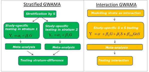
Assuming the large-scale GWAMA configuration, G x S interaction effects can either be modelled by conducting a stratified GWAMA or by conducting an interaction GWAMA (Figure 3). In the following, considerations are limited to linear regression models involving continuous phenotypes Y, additively modeled genotypes G and dichotomous stratification variables S.

Figure 3. Modelling G x S interaction effects in large-scale GWAMAs.

The interaction GWAMA model – involving a single dichotomous environmental variable S - is given by the regression model that includes a G x S interaction term:

𝑌 = 𝛼 + 𝛽_𝐺𝐺 + 𝛽_𝑆𝑆 + 𝛽_𝐺𝑥𝑆𝐺𝑥𝑆 + 𝜀, 𝜀~𝑁(0, 𝜎²) (3).

Here, 𝛽_𝐺 is the genetic effect on the phenotype, 𝛽_𝑆 the effect of the stratification variable on the phenotype, and 𝛽_𝐺𝑥𝑆 the G x S interaction effect on the phenotype. For each SNP, each study fits the interaction model and obtains study-specific effect and interaction estimates with standard errors. Pooled genetic effect estimates bG and pooled G x S interaction effect estimates b_GxS are obtained from inverse-variance weighted meta-analyses of the respective study-specific estimates. Testing for G x S interaction effects can be accomplished by performing a t test on the pooled interaction estimates b_GxS.

Assuming two strata, the stratified GWAMA model involves two linear regression models (one for each stratum):

𝑌₁=∝₁+ 𝛽₁𝐺₁+ 𝜀₁, 𝜀₁~𝑁(0, 𝜎₁²)

𝑌₂=∝₂+ 𝛽₂𝐺₂+ 𝜀₂, 𝜀₂~𝑁(0, 𝜎₂²) (4).

The stratification is done by a dichotomous variable that separates each study sample into two subgroups. A stratum-specific regression model is fitted for each SNP and in each study separately yielding stratum-specific effect estimates with standard errors. Pooled stratum- specific genetic effect estimates, b₁ and b₂, are obtained from stratum-specific inverse- variance weighted meta-analyses. Testing for G x S interaction can be accomplished by testing the pooled stratum-specific estimates for difference (Randall et al., 2013).

1.5.2 Methods to account for and to identify gene-strata interaction effects

When defining methods to tackle G x S interaction effects, it is extremely important to distinguish between two major aims: On the one hand one might be interested in methods to identify SNP effects while accounting for interaction; on the other hand one might be interested in detecting the interaction per se for a specific locus.

Several methods have been described that improve power to identify SNP effects while accounting for interaction. For example, the simple approach of stratum-specific association testing (using the pooled stratum-specific estimates gathered from a stratified GWAMA) has been shown to improve power to find stratum-sensitive variants (Behrens et al., 2011). Other methods focus on the detection of joint (main + interaction) effects (Kraft, Yen, Stram, Morrison, & Gauderman, 2007) and those methods have recently been extended to the interaction GWAMA model (Manning et al., 2011) and to the stratified GWAMA model (Aschard, Hancock, London, & Kraft, 2010). Importantly, a significant joint effect does not automatically imply significant interaction. Disentangling whether a significant joint effect is due to main effect, interaction effect, or both, has to be outlined additionally.

There is some concern as to whether this can be done using the obtained main and interaction estimates from the data set that was used for discovery of joint effects.

Similarly, several methods have been described that aim at identification of gene- environment interaction effects. However, most of the reported methods are tailored for single studies with dichotomous disease outcomes (D. Li & Conti, 2009; Mukherjee &

Chatterjee, 2008; Piegorsch, Weinberg, & Taylor, 1994). Their applicability to continuous outcomes, and to the large-scale GWAMA setting, may be limited and has not yet been shown. A structured and detailed comparison of GWAMA approaches - aiming at identification of G x S interaction effects for continuous outcomes - with regards to type 1 error and power while considering varying types of interaction effects, study designs, and statistical tests, is lacking. For example, for the GIANT sex-stratified GWAMAs for WHR_adjBMI, it is not yet clear what screening approach is optimal to identify loci with significant sex- difference.

1.6 Objectives

Genome-wide association meta-analyses (GWAMAs) of obesity traits have proven to successfully pinpoint associated genetic variants. For example, in 2010, a large-scale GWAMA for WHR_adjBMI (waist-hip ratio adjusted for BMI, as a measure of central obesity) detected significant associations at 14 genetic loci.

Interestingly, seven of the 14 loci displayed significantly stronger genetic effects in women than in men. Remarkably, these sex-differences were detected for variants that were initially selected for overall (sex-combined) association. Yet, a systematic genome-wide screen to identify variants displaying sex-difference was lacking and the dimension of sex- differences in the genetics of anthropometric traits was unknown. Sex-stratified GWAS data had already been available at that time for most studies involved in the 2010 GIANT consortium meta-analyses. However, there was uncertainty as to what screening approach should be applied ideally to identify sex-difference from the available sex-stratified GWAS. A systematic methodological evaluation of approaches with regard to type 1 error and power to identify sex-difference was lacking.

Additionally, two further GIANT projects were in planning that aimed at the identification of other stratum-differences in genetic effects for obesity traits. One project started to conduct a smoking-stratified GWAMA (to identify differences in genetic effects between current smokers and non-smokers), the other started to conduct an activity-status stratified GWAMA (to identify differences in genetic effects between physically active and inactive individuals). In contrast to the balanced sex-stratified GWAMA design (similar numbers of men and women involved) these two projects reflect an unbalanced design: For example there are fewer smokers than non-smokers available for the analyses. The impact of unequal stratum sizes on the identification of stratum-difference had not been clear.

A further project was in planning that aimed to identify age- and sex-dependent genetic effects for obesity traits. The rationale behind this analysis was that body shape changes in women upon menopause (approximately at 50 years of age) resulting in a more android body shape that is less different from men. Age- and sex-stratified GWAMAs (four strata: younger men, older men, younger women, older men; age stratified at 50 years of age) were supposed to be employed to investigate potential 3-way G x AGE x SEX interaction effects. But again, there was uncertainty as to what approach should be applied to ideally find such 3-way interaction effects from the age- and sex-stratified GWAMA results.

Finally, large-scale stratified GWAMAs are high-dimensional complex analyses. For example, GIANT involves multiple stratified GWAS results (each carrying millions of SNP- specific association test results) from hundreds of studies, for multiple genotyping platforms and imputation reference panels, for multiple anthropometric and obesity traits as well as for multiple environmental stratification variables. This involves the handling of thousands of individual GWAS result files - each with millions of SNP-specific association testing results.

Ensuring validity of each single GWAS result and of the obtained GWAMA result requires extended quality control procedures and software that is able to cope with thousands of large association result files. Furthermore, software was required that provides extended statistical

To address the described research gaps, the four main objectives of this work were defined as follows:

1. Develop and improve stratified GWAMA approaches to identify difference in genetic effects between two strata (chapter 2).

2. Extend methods to identify 3-way G x AGE x SEX interaction effects from an age- and sex-stratified GWAMA (chapter 3).

3. Apply optimized methods to stratified GWAMA results from the GIANT consortium (chapter 4).

4. Develop software to facilitate quality control and statistical evaluation of stratified GWAMAs (chapter 5).

2 Stratified GWAMA approaches to screen for difference between two strata

Generally, stratum-difference is defined as the difference in genetic effects between two strata (e.g., men and women). The overarching aim of the following chapter is to provide a systematic methodological evaluation of stratified GWAMA screening approaches that are based on two strata and aim at identifying stratum-difference.

Generally, an approach is defined here as a combination or concatenation of multiple statistical tests (i.e., steps) that are applicable to stratified GWAMA outcomes and that are implemented in one or two independent data sets (i.e., stages). Relevant statistical tests are introduced and a systematic scheme of approaches is presented.

The performance of the approaches was compared by simulation-based estimation of type 1 error and by analytical computations of power. Varying realistic scenarios were considered and an attempt to recommend approaches - based on study design and based on type of stratum-difference - was made.

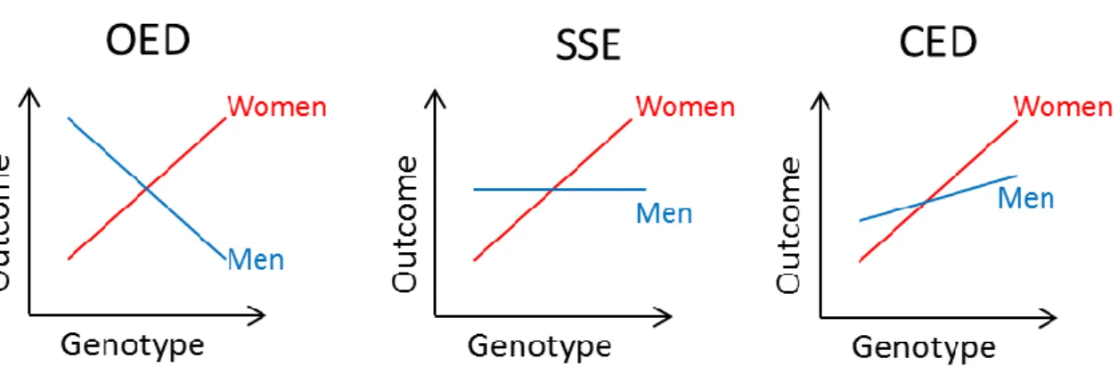
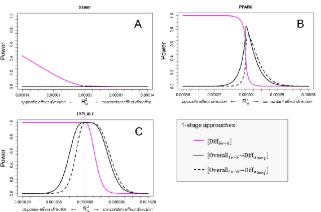
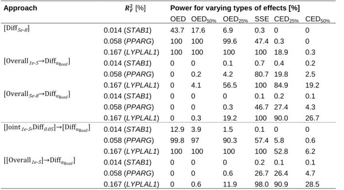
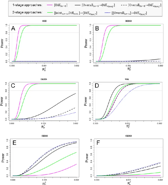
Three general types of stratum-difference were defined (Figure 4). Assuming an effect in one stratum (e.g., women), the effect in the other (i.e., men) may be opposite (opposite effect direction, OED), lacking (single-stratum effect, SSE) or be concordant but less pronounced (concordant effect direction, CED).

Figure 4. Different types of stratum-specific effects on the example of sex-difference (assuming a positive effect in women).

2.1 Materials and Methods

The following chapters describe the prerequisites of the methodological evaluation of stratified GWAMA approaches to identify stratum-difference.

After presenting general assumptions (chapter 2.1.1), relevant statistical tests are introduced (chapters 2.1.2 and 2.1.3) and then used to construct several screening approaches (chapter 2.1.4). A systematic scheme of approaches was developed that is utilized to compare performance (type 1 error and power) between approaches. Details about the simulation-based type 1 error evaluation (chapter 2.1.5), the derivation of analytical power formulae as well as about the analytical power computations (chapter 2.1.6), are presented.

2.1.1 Assumptions and definitions

In the following, considerations are based on a stratified GWAMA model involving two strata (as given by equation (4)), a continuous phenotype (e.g., WHR_adjBMI), a dichotomous stratification variable (e.g., sex) and additively modeled genotypes. It is assumed that the stratified GWAMAs have already been conducted so that pooled stratum-specific effect estimates and standard errors are available.

Stratum-specific continuous phenotypes are assumed to follow identical normal distributions, 𝑌₁~𝑁(𝜇_𝑌, 𝜎_𝑌²) and 𝑌₂~𝑁(𝜇_𝑌, 𝜎_𝑌²).

Similarly, stratum-specific additively modeled genotypes 𝐺₁ and 𝐺₂ are assumed to follow equal genotype distributions across strata implying identical minor allele frequencies (MAF) and thus identical genotype means 𝜇_𝐺= 𝜇_𝐺1= 𝜇_𝐺2 = 2𝑀𝐴𝐹 and identical genotype variances 𝜎_𝐺²= 𝜎_𝐺1² = 𝜎_𝐺2² = 2𝑀𝐴𝐹(1 − 𝑀𝐴𝐹). This assumption builds upon the assumption of random mating between strata.

Importantly, the GWAMAs are assumed to only include GWAS from similar populations. Similar populations involve equal MAF across studies. This implies equal genotype distributions and homogeneous genetic effects across studies. Based on this assumption, meta-analysis of multiple study-specific SNP summary statistics yields approximatively identical results as a ‘mega-analysis’ of all individuals in one single large study (Evangelou & Ioannidis, 2013). Therefore, the meta-analysis concept was ignored in the following and one large study involving all individuals was assumed.

A sex-stratified GWAMA is defined as men- and women-specific GWAMA involving equal sex-specific sample sizes, 𝑛_𝑀= 𝑛_𝐹. For a general stratified GWAMA, stratum-specific sample sizes are allowed to be unequal, 𝑛₂= 𝑓 ∙ 𝑛₁, where f is the ratio of stratum 2 sample size to stratum 1 sample size (f = 1 for the sex-stratified GWAMA setting).

2.1.2 Testing for stratum-difference

To investigate stratum-difference given a stratified GWAMA model with two strata, a difference test can be conducted that compares the pooled stratum-specific genetic effect estimates (𝐻₀: 𝑏₁= 𝑏₂):

𝑍𝐷𝑖𝑓𝑓 = 𝑏₁−𝑏₂

√𝑠𝑒(𝑏₁)²+𝑠𝑒(𝑏₂)²

~𝑁(0,1) |𝐻0 (5).

Assuming the null hypothesis being true, the z statistic follows a standard normal distribution.

The z test yields the difference P-Value P_Diff.

Under the assumption of independent samples, unrelated subjects and no latent covariate interacting with S (the stratification variable), the difference test is mathematically equivalent to testing the pooled G x S interaction estimate bGxS obtained from an interaction GWAMA model (as given by equation (3)).

In order to correct for potential correlation between stratum-specific effects b₁ and b₂, an alternative of the difference test can be employed:

𝑍𝐷𝑖𝑓𝑓= 𝑏₁−𝑏₂

√𝑠𝑒(𝑏₁)²+𝑠𝑒(𝑏₂)²− 2𝑟 ∙𝑠𝑒(𝑏₁) ∙ 𝑠𝑒(𝑏₂)

~𝑁(0,1) |𝐻0 (6).

Here, r denotes the Spearman rank correlation between b₁ and b₂ that is estimated from the two stratum-specific genome-wide data sets. For example, such correlation could stem from family studies that contribute related individuals to both strata, e.g., brothers and sisters contributing to a sex-stratified GWAMA. Such relatedness would result in ‘less different’

effect estimates, increased type 2 error and deflated PDiff. The correction should only be used with genome-wide data sets that allow for accurate estimation of the correlation.

In the following, unrelated subjects across strata are assumed and stratum-specific estimates b₁ and b₂ are assumed to be uncorrelated.

2.1.3 Statistical tests to filter stratified GWAMA data sets prior to difference testing

Often in GWAMA literature, the difference (or interaction) testing is limited to SNPs that were initially selected using other statistical tests, such as stratum-specific, overall or joint (main + interaction) association tests (Heid et al., 2010; Manning et al., 2012; Randall et al., 2013).

For example, Heid and colleagues primarily screened for overall (strata-combined) associated variants for WHRadjBMI, and subsequently tested the identified (overall associated) SNPs for sex-difference.

In order to construct stratified GWAMA approaches that reflect such analyses, three filtering tests are considered that can directly be applied to stratified GWAMA outcomes b₁

 A stratified test can be performed to infer whether any of the stratum-specific effects is associated with the phenotype (𝐻₀: 𝑏₁= 0 ∧ 𝑏₂= 0): The stratified test employs two t tests, 𝑇₁= 𝑏₁/𝑠𝑒(𝑏₁)~𝑡(𝑛₁− 2)|𝐻₀ and 𝑇₂= 𝑏₂/𝑠𝑒(𝑏₂)~𝑡(𝑛₂− 2)|𝐻₀, that yield stratum- specific association P-Values, P₁ and P₂. Finally, a stratified association P-Value is defined as PStrat = 2*min(P1,P2), which is corrected for the multiple testing of two strata.

 An overall test can be performed to infer whether the overall (strata-combined) effect is associated with the phenotype (𝐻₀: 𝑏_{𝑂𝑣𝑒𝑟𝑎𝑙𝑙} = 0):

𝑇_{𝑂𝑣𝑒𝑟𝑎𝑙𝑙} = 𝑏_{𝑂𝑣𝑒𝑟𝑎𝑙𝑙}

𝑠𝑒(𝑏_{𝑂𝑣𝑒𝑟𝑎𝑙𝑙})^~𝑡(_{𝑛𝑂𝑣𝑒𝑟𝑎𝑙𝑙− 2})|_𝐻0 (7), where n_Overall is the strata-combined sample size (𝑛_{𝑂𝑣𝑒𝑟𝑎𝑙𝑙}= 𝑛₁+ 𝑛₂), and where b_Overall and se(bOverall) are the overall genetic effect estimate with standard error that are obtained from inverse-variance weighted meta-analysis of the two strata:

𝑏_{𝑂𝑣𝑒𝑟𝑎𝑙𝑙}=𝑏₁⁄𝑠𝑒(𝑏₁)²+ 𝑏₂⁄𝑠𝑒(𝑏₂)² 1 𝑠𝑒(𝑏⁄ ₁)²+ 1 𝑠𝑒(𝑏⁄ ₂)²

𝑠𝑒(𝑏_{𝑂𝑣𝑒𝑟𝑎𝑙𝑙}) = √ 1

1 𝑠𝑒(𝑏⁄ ₁)²+ 1 𝑠𝑒(𝑏⁄ ₂)²

(8).

The t test yields the overall association P-Value P_Overall.

 A joint test can be performed to infer whether the joint effect of both the main effect and the interaction effect is associated with the phenotype (𝐻₀: 𝑏_𝐺 = 0 ∧ 𝑏_𝐺𝑥𝑆= 0):

𝐶_{𝐽𝑜𝑖𝑛𝑡} = ( 𝑏₁ 𝑠𝑒(𝑏₁))

2

+ ( 𝑏₂ 𝑠𝑒(𝑏₂))

2

~𝜒²(2) |𝐻₀ (9).

The chi-square test yields the joint-test P-Value P_Joint. The joint test based on stratum- specific effects originates from the joint test that simultaneously tests for main and interaction effects in an interaction model (Kraft et al., 2007). The two versions of the joint tests are identical, if the G x S interaction is modelled with dichotomized S (Aschard et al., 2010).

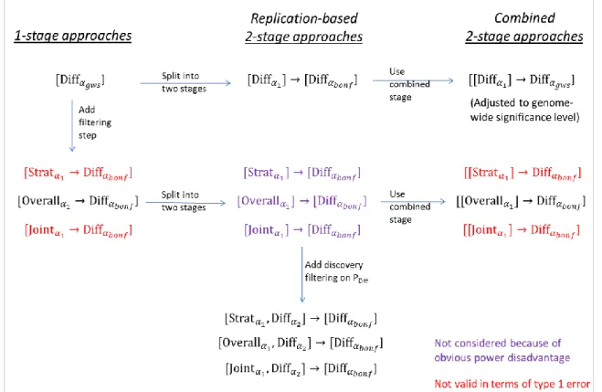
2.1.4 A systematic scheme of stratified GWAMA approaches to identify stratum-difference

The introduced statistical tests are used to construct several stratified GWAMA approaches, each of which aims at screening for variants with significant stratum-difference. Generally, an approach is designed with multiple steps (statistical tests). The last step of each approach is to test for difference. The stratified, the overall, or the joint test, are solely employed for filtering the genome-wide data sets prior to the difference testing. Multiple steps are either implemented within a single data set (1-stage design) or implemented within two independent data sets (discovery and replication data set, 2-stage design). For the 2-stage approaches, the filtering is conducted in the discovery stage data and difference testing is

either conducted using the replication stage data only (replication-based 2-stage approach) or using the combined (discovery + replication) stage data (combined 2-stage approach).

To distinguish between approaches, a general notation is introduced: [.] indicates a stage and ‘Test_α’ denotes the step-specific test and the respective -level. For example, [Overall_α1→Diff_αdiff] denotes a 1-stage approach that involves filtering on POverall < 1 and testing the selected SNPs for difference and that employs identical subjects for both steps.

Alternatively, [Overall_α1]→[Diff_αdiff] (or [[Overall_α1]→Diff_αdiff] ) denotes the respective replication-based 2-stage (or combined 2-stage) approach that involves testing the selected SNPs for difference using the replication (or combined discovery + replication) subjects.

Based on this notation, a systematic scheme of the considered approaches was developed and summarized in Figure 5.

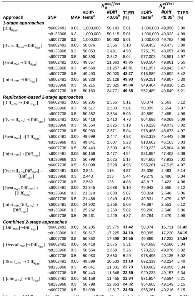
Figure 5. Systematic scheme of stratified GWAMA approaches to identify stratum-difference (gws:= 5 x 10^-8; 1 = -level for the filtering step; 2 = -level for the additional discovery filter on difference; _Bonf = Bonferroni-corrected -level).

Generally, all of the considered approaches aim at using Bonferroni-corrected - levels for the final difference test, Bonf = 0.05/M, where M is the number of independent difference tests performed.

The most intuitive approach is the 1-stage approach [Diff_αgws], which screens for difference at a genome-wide significance level, _Bonf = _gws = 5 x 10^-8 (= 0.05/10⁶, Bonferroni- corrected for an approximate number of one million independent tests). The genome-wide significance level is a well-established screening threshold in GWAS of HapMap imputed data (Johnson et al., 2010).

Extending this intuitive approach to the 2-stage design, the difference test can either be implemented as a replication-based 2-stage approach [Diff_α1]→[Diff_αBonf] or as a combined 2-stage approach [[Diff_α1]→Diff_αgws]. Due to employing a single statistical test (difference test), the design of the two approaches is similar to a general 2-stage GWAMA approach that screens for overall SNP association and for which the implementation into various 2-stage designs has been discussed before (Skol, Scott, Abecasis, & Boehnke, 2006). For the replication-based 2-stage approach [Diff_α1]→[Diff_αBonf], it is well known that significance for the final test can be attained using a Bonferroni-corrected -level that is corrected for the independent number of SNPs tested (selected from the discovery data). For the combined (discovery + replication) 2-stage approach [[Diff_α1]→Diff_αgws], overlapping subjects between ‘discovery stage SNP selection’ and ‘combined stage difference testing’

are used, which is why the -level of the final difference test has to be adjusted to the genome-wide significance level in order to yield valid type 1 error rates.

Further approaches are considered that involve initial filtering on stratified, overall or joint association tests. Their implementation into 1- and 2-stage designs has to be validated with regards to type 1 error and their impact on power to find stratum-difference has to be investigated.

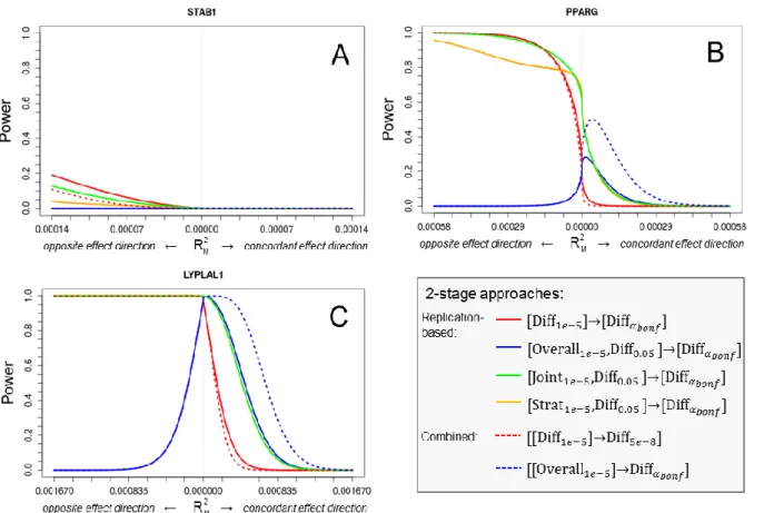
For the replication-based 2-stage approaches, an additional discovery filter on difference is considered, e.g., for approach [Joint_1e-5,Diff_0.05]→[Diff_αBonf], see Figure 5. The rationale behind this filter is that it increases power for the replication stage difference test by (i) lowering the multiple testing burden due to taking less SNPs forward, and (ii) by focusing on variants that are more likely to be truly dimorphic than variants that do not display any difference in discovery.

Practically, common stratified GWAMA projects aim at identification of any type of stratum-difference and it is likely that the optimal approach varies by type of stratum- difference. Thus, it is expected that multiple approaches have to be outlined in parallel in order to efficiently identify the various types of stratum-difference. In fact, this necessitates an additional multiple-testing correction for the final difference tests that have to be corrected for the number of screening approaches. Notably, each screening approach itself already employs a conservative Bonferroni-correction. Thus and in order to avoid overly conservative correction, such ‘final’ correction is ignored in the following.

Technically, single genetic loci contain multiple correlated SNPs that are all located nearby within a specific region. To avoid overly conservative control of the final difference test, the filtered subsets of SNPs are clumped into independent regions and region-wide lead-SNPs are selected that are independent of other lead-SNPs (from other regions).

Commonly used clumping criteria are LD-based (e.g., pairwise r² > 0.2, between SNPs of a specific region) or distance-based (e.g., distance < 500KB, pairwise between SNPs of a specific region). In the following, considerations are limited to a distance-based clumping criterion: distance < 500KB. The lead-SNP of a specific region is defined as the SNP with the lowest P-Value across all SNPs of the respective region. Importantly, the independent lead- SNPs are those that are put forward and are tested for difference in the final step. The total number of selected lead-SNPs is denoted as M in the following (as introduced before). To correct for the multiple difference testing of M independent lead SNPs, the -level of the difference test undergoes a Bonferroni–correction, Bonf = 0.05/M (except for approaches [Diff_{α𝑔𝑤𝑠}] and [[Diff_α1]→Diff_{α𝑔𝑤𝑠}] that employ genome-wide significant -levels for the final difference test).

2.1.5 Simulation-based evaluation of type 1 error

A simulation-based evaluation of type 1 error rates was performed for all of the defined approaches. Methodological details of the simulations are described in the following.

Simulated data sets were created that follow the null hypothesis of ‘No difference in genetic effects between strata’ (𝐻₀: 𝑏₁= 𝑏₂). More specifically, two versions of the null hypothesis were created: One assumes lack of stratum-specific effects (𝐻₀^{𝑛𝑜𝑒𝑓𝑓𝑒𝑐𝑡}: 𝑏₁= 𝑏₂ = 0), the other assumes identical (unequal zero) stratum-specific effects (𝐻₀^{𝑒𝑓𝑓𝑒𝑐𝑡}: 𝑏₁= 𝑏₂ ≠ 0).

First, real genotypes were obtained for 1,500 men and 1,500 women from the KORA study (Wichmann, Gieger, Illig, & Group, 2005) for one well-imputed SNP: rs8138968 (MAF = 0.3).

Second, simulated sex-specific phenotypes (for the 1,500 men and 1,500 women) were created according to Y~N(0,1) (to reflect 𝐻₀^{𝑛𝑜𝑒𝑓𝑓𝑒𝑐𝑡}), and according to Y|G=0~N(0,1), Y|G=1~N(b_80%,1) and Y|G=2~N(2*b_80%,1) (to reflect 𝐻₀^{𝑒𝑓𝑓𝑒𝑐𝑡}). Herewith, b_80% corresponds to the minimum effect size detectable with 80% power by 1,500 samples (at  = 0.05), and G=0, G=1 or G=2 denote the group of individuals carrying 0, 1, or 2 minor alleles, respectively. Using G*Power, b_80% was estimated to be 0.111 for rs8138968 (Faul, Erdfelder, Buchner, & Lang, 2009).

Third, for each null hypothesis, the simulated phenotypes were sex-specifically tested for association with the real SNP genotypes. Men- and a women-specific genetic effect