Regensburger
DISKUSSIONSBEITRÄGE zur Wirtschaftswissenschaft
University of Regensburg Working Papers in Business, Economics and Management Information Systems
Matrix Box-Cox Models for Multivariate Realized Volatility
Roland Weigand March 21, 2014
Nr. 478
JEL Classification: C14, C32, C51, C53, C58
Key Words: Realized covariance matrix, dynamic correlation, semiparametric estimation, density forecasting
Roland Weigand is a researcher at the Institute of Employment Research, 90478 Nuremberg, Germany, and
Matrix Box-Cox Models for Multivariate Realized Volatility
Roland Weigand∗
Institute for Employment Research (IAB), D-90478 Nuremberg
March 2014
Abstract. We propose flexible models for multivariate realized volatility dynamics which in- volve generalizations of the Box-Cox transform to the matrix case. The matrix Box-Cox model of realized covariances (MBC-RCov) is based on transformations of the covariance matrix eigenvalues, while for the Box-Cox dynamic correlation (BC-DC) specification the variances are transformed individually and modeled jointly with the correlations. We estimate transfor- mation parameters by a new multivariate semiparametric estimator and discuss bias-corrected point and density forecasting by simulation. The methods are applied to stock market data where excellent in-sample and out-of-sample performance is found.
Keywords. Realized covariance matrix, dynamic correlation, semiparametric estimation, density forecasting.
JEL-Classification. C14, C32, C51, C53, C58.
∗Phone: +49 911 179 3291, E-Mail: roland.weigand@iab.de
This research has partly been done at the Institute of Economics and Econometrics of the University of Re- gensburg. The author is very grateful for helpful comments by Rolf Tschernig, Enzo Weber and participants of the Humboldt–Copenhagen Conference on Financial Econometrics 2013. Support by BayEFG is gratefully acknowledged.
1 Introduction
Dynamic modeling of multivariate financial volatility has recently gained significant interest.
On the one hand, it constitutes an essential part of portfolio decisions, in empirical asset pricing models and for derivative analysis. On the other hand, recent financial crises have accentuated the importance of quantifying systemic risk. The latter also requires multivariate rather than univariate models. Such models require a precise measure of the otherwise latent asset variance and covariance processes and a framework for modeling the dynamics. Precise measures are available due to recent and significant achievements on multivariate realized financial volatility modelling; see, e.g., Andersen et al. (2003) and Barndorff-Nielsen and Shephard (2004).
There are several approaches for modeling covariance dynamics. A prominent model class is based on conditionally Wishart distributed processes (see, e.g., Golosnoy et al.; 2012). Al- ternatively, linear vector time series models are applied to specific transformations of realized covariance matrices. The latter approach has the advantage of simplicity; model estimation, checking and inference is implemented in econometric software packages, while suitable ways of handling high-dimensional panels of time series are well-established. Various transformations have recently been suggested: Chiriac and Voev (2011), for instance, use the elements of a triangular matrix square-root transform, while the matrix logarithm has been considered by Bauer and Vorkink (2011) as well as Gribisch (2013). For these models, fitted covariance matri- ces and out-of-sample forecasts are automatically positive definite through the corresponding retransformations.
Likewise, approaches that separate variance and correlation dynamics, so called dynamic correlation (DC) models have been a fruitful direction of research. With appropriate factor or panel structure assumptions, Golosnoy and Herwartz (2012) model the z-transformed realized correlations (cf. (6) below). Correlation eigenvalues along with locally constant eigenvectors, sampled at different frequencies, are used by Hautsch et al. (2014). Separate realized variance and correlation dynamics in mixed frequency models are also investigated by Halbleib and Voev (2011).
In the univariate time series literature, where transformation-based methods have a long tradition, the model of Box and Cox (1964) has become popular to find a suitable transform prior to ARIMA analysis (Box and Jenkins; 1970). Similar approaches were used for univariate volatility modeling, e.g., by Higgins and Bera (1992), Yu et al. (2006), Zhang and King (2008)
and Goncalves and Meddahi (2011).
We propose two flexible models in the spirit of Box and Cox (1964) for the dynamic mul- tivariate realized volatility setup. Both generalize the univariate Box-Cox transform to the matrix case and contain several well-known transforms as special cases. The matrix Box-Cox model of realized covariances (MBC-RCov) is based on transformations of the covariance ma- trix eigenvalues. On the other hand, for the Box-Cox dynamic correlation (BC-DC) model, the variances are transformed individually and modeled together with the z-transformed cor- relations.
We introduce a semiparametric estimator of the transformation parameters in the multi- variate setup by generalizing the univariate approach of Proietti and L¨utkepohl (2013). It does not require the specification of a dynamic model and makes a computationally simple two-step approach feasible. A simulation-based forecasting procedure is presented to reduce the bias of the na¨ıve re-transform forecasts. Simulated paths of the realized volatilities may also be used to obtain density forecasts of the daily returns which will often be the aim of studying covariance matrix dynamics.
We apply these methods to the data set of Chiriac and Voev (2011) and find that a sparse vector autoregressive vector moving average (VARMA) specification provides a reasonable fit to the transformed series. A pseudo out-of-sample forecast comparison is conducted, where the BC-DC specification either with estimated transformation parameters or restricted to the loga- rithmic case emerges as favorable in practice. Bias correction provides significant improvements over the na¨ıve forecasts. Notably, also the conditional Wishart models as popular benchmarks are outperformed by our transformation-based approach. These results are robust to different dynamic specifications and remain qualitatively intact for most of the loss functions recently used for evaluations of this kind.
The paper is organized as follows: In section 2 the new models are introduced. Parameter estimation and forecasting is described in sections 3 and 4, respectively. Section 5 presents the estimation results, while section 6 contains the out-of-sample forecast evaluation. Section 7 concludes.
2 Multivariate Box-Cox volatility models
In univariate regression and time series models, the Box-Cox transformation (Box and Cox;
1964) has been applied to obtain a linear, homoscedastic specification for the transformed dependent variable. For a scalarx >0, it is parameterized byδ and given by
h(x;δ) =
xδ−1
δ forδ6= 0, log(x) forδ= 0.
(1)
For specific choices ofδ, the transform corresponds to a linear mapping of the raw series (δ= 1) or of various popular transforms such as the square root (δ= 0.5), the logarithm (δ= 0) and the inverse (δ =−1). The reverse transform is given by
h−1(y;δ) =
(δy+ 1)1δ forδ6= 0, exp(y) forδ= 0,
(2)
which is defined fory >−1δ ifδ >0 and fory <−1δ ifδ <0, and gives strictly positive values.
2.1 The matrix Box-Cox model of realized covariances
To generalize the Box-Cox method for modeling covariance matrices we define a matrix version of the latter, the matrix Box-Cox (MBC) transform. For a positive definite (k×k) covariance matrix Xt, and t = 1,2, . . . denoting time periods, we suggest to apply Box-Cox transfor- mations to the eigenvalues of Xt, each with a distinct transformation parameter collected in δ= (δ1, . . . , δk)0,
Yt(δ) :=H(Xt;δ) =Vt
h(λ1t;δ1) 0 . . . 0 0 h(λ2t;δ2) . .. ...
... . .. . .. 0
0 . . . 0 h(λkt;δk)
Vt0. (3)
Hereλ1t≥. . .≥λkt≥0 are the eigenvalues of Xt,h(λit;δi), i= 1, . . . , k, are their univariate Box-Cox transforms andVtdenotes the matrix of eigenvectors of Xt.
To understand the consequences of the MBC approach for modelling covariance matrices,
it is useful to consider the inverse transformation, applied to a symmetric (k×k) matrixYt,
H−1(Yt;δ) =Vt
h−1(λy1t;δ1) 0 . . . 0 0 h−1(λy2t;δ2) . .. ...
... . .. . .. 0
0 . . . 0 h−1(λykt;δk)
Vt0. (4)
Here, byλyjt,j= 1, . . . , k, we denote the eigenvalues ofYt, whileVtcontains the eigenvectors of bothYt andH−1(Yt;δ), which remain unaffected by the transform. Notably, when the inverse MBC transform is well defined and applied to a symmetric matrix, the re-transformed fitted or forecasted matrices are always positive definite.
The reverse Box-Cox transform is not always well-defined, however. As mentioned below (2), existence ofh−1 and hence ofH−1 requires that the eigenvalues satisfy certain restrictions, namely λyjt(δj) > −δ1
j for δj > 0 and λyjt(δj) < −δ1
j for δj < 0. This requirement limits the set of feasible values ofδ for a given sequence of matrices (e.g., forecasts) to which the inverse transform has to be applied. Our empirical results for stock market data suggest that this potential drawback may be irrelevant as long as the applied transformation parameters are not chosen grossly at odds with estimates from the data (i.e. forδj >−0.25 in our application).
As in the univariate setup, the matrix transform contains as special cases linear combina- tions of the raw matrix entries (δ1 = δ2 = . . . = δk = 1), of the (symmetric) matrix square rootδ1 = δ2 =. . . =δk = 0.5), of the matrix logarithm (δ1 =δ2 =. . . =δk = 0) and of the inverse (δ1=δ2 =. . .=δk=−1). It thus incorporates several empirically relevant approaches to covariance modeling within a common framework. We call this approach for modeling and forecasting multivariate realized volatility the matrix Box-Cox model of realized covariances (MBC-RCov).
For all periods t = 1, . . . , T, the MBC-transform is applied to the realized covariance matrices Xt for an appropriate vector of parameters δ. In this way we obtain a sequence of symmetric matrices Yt(δ) from which only the lower triangular elements (including the main diagonal) need to be modeled. A time series model is thus fitted only to the k(k+ 1)/2-
dimensional vector processyt(δ) := vech(Yt(δ))1. For generality, we assume a linear process yt(δ) =
∞
X
j=0
Ψj(θ)ut−j, ut∼IID(0; Σu), (5) with Ψ0 =I. We let θ as well as Σu consist of unknown parameters. Specific models will be considered in the empirical application in section 5. Here, we apply diagonal vector autoregres- sive moving average (VARMA) models as well as fractionally integrated VARMA (VARFIMA) and multivariate heterogeneous autoregressive (HAR) models.
2.2 The Box-Cox dynamic correlation model
As an alternative to the matrix version of the Box-Cox transform, we consider a decompo- sition of variances and correlations. Applying the Box-Cox transform to the individual as- set variances we introduce the Box-Cox dynamic correlation (BC-DC) model. In the spirit of dynamic conditional correlation models (Engle; 2002), we write Xt = DtRtDt, where Dt = diag(p
X11,t, . . . ,p
Xkk,t) is a diagonal matrix containing the univariate realized stan- dard deviations while Rt is the sequence of realized correlation matrices. Applying Fisher’s z-transformation
R˜ij,t:= 1
2log1 +Rij,t
1−Rij,t (6)
to the correlations has several advantages as compared to using the raw correlations (see Golosnoy and Herwartz; 2012), so that we propose modelling the vector time series
zt(δ) :=g(Xt;δ) := (h(X11,t;δ1), . . . , h(Xkk,t;δk),R˜21,t,R˜31,t, . . . ,R˜k k−1,t)0, (7) as a linear process analogous to (5).
The inverse BC-DC transform g−1, when applied to forecasted zT+h, yields positive vari- ances due to the inverse Box-Cox and correlations in the range (−1; 1) due to the inverse Fisher transform. In contrast to the matrix Box-Cox approach, positive definiteness is not guaranteed for k > 2, however.2 Whenever positive definiteness fails, it has to be enforced and a well-
1A different strategy would be to fit a model directly to the transformed eigenvalues and free elements of the eigenvectors, analogously to the approach of Hautsch et al. (2014). They find that the eigenvectors are rather noisy and unstable at daily frequency which is not the case for our vech-transformation.
2As a counterexample where the unrestricted forecasts do not yield a valid correlation matrix, considerk= 3 and suppose that the inverse Fisher transform givesR12,t=R13,t= 0.8 along withR23,t=−0.8. The quadratic formγ0Rtγis negative, e.g., forγ= (1,−1,−1)0.
conditioned matrix must be obtained by some sort of eigenvalue trimming or shrinkage proce- dure. Positive definiteness, however, is not problematic empirically even in high-dimensional stock market applications for z-transformed correlation matrices as the results of Golosnoy and Herwartz (2012) suggest. Compared to the MBC-RCov approach, the estimated dynamics of the linear model (5) fitted to zt(δ) are easily interpreted. The matrix Σu, for example, pro- vides guidance about the extent of instantaneous co-movement within groups of variances or correlations but also between correlations and variances. Dynamic spill-overs may be modeled by non-diagonal specifications for Ψj(θ).
In addition to enabling a linear homoskedastic specification, the Box-Cox transform has originally been introduced to reduce the deviation from normality of the involved variables or model residuals. However, for the univariate transform (1) it holds that h(x;δ) > −1δ for δ >0 and h(x;δ) < −1δ for δ <0. Due to its bounded support, hence, the BC-transformed variable cannot literally be Gaussian whenever δ 6= 0; see, e.g., Amemiya and Powell (1981).
Merits of the transform even in cases where Gaussianity fails have been pointed out by Draper and Cox (1969). Although in the matrix case the MBC-transformed series are not individually bounded, the same logic implies that the MBC- and BD-DC-transformed series cannot be exactly multivariate normal. We do not need the Gaussianity assumption at this stage but empirically assess whether the transformed data are at leastapproximately Gaussian later on.
3 Semiparametric estimation of the transformation parameter
In this section we discuss semiparametric estimation of the vector of transformation parame- ters δ. Among others, Han (1987) has proposed a semiparametric approach to estimate the transformation parameter of a single variable. Likewise, the recently developed estimator of Proietti and L¨utkepohl (2013) for time series data does not involve specifying a parametric dynamic model. It is computed by minimizing a frequency-domain estimate of the prediction error variance of the transformed series. In the following, we generalize their approach to multivariate BC-DC and MBC-RCov setups. For the BC-DC model, our multivariate method provides a potentially more efficient estimator than applying the univariate estimator to allk variance series individually and allows to impose cross-equation restrictions. Moreover, in the MBC-RCov context, estimation is inherently multivariate and hence the existing semiparamet- ric approaches would not be applicable without modifications.
In multivariate (vector) Box-Cox regression models, where each of the k nonnegative en- dogenous variables, say realized variances (X11,t, . . . , Xkk,t)0, are transformed individually, the standard estimation strategy has been maximum likelihood under the auxiliary assumption of Gaussian transformed variables; see, e.g., Velilla (1993). Maximum likelihood estimation can be straightforwardly extended to the MBC-RCov model, as we outline in Appendix A. In case of dynamic models, the likelihood is simultaneously maximized with respect to both, the dynamic and the transformation parameters. In contrast, our approach allows the researcher to proceed in two steps: After the estimation of the transformation parameters, which involves a k-dimensional optimization for both the BC-DC and MBC-RCov approach, the dynamic model specification and estimation is carried out for the transformed series as ifδ was known.
To sketch our semiparametric approach for a generic k-dimensional vector processxtwith strictly positive elements, we consider the Jacobian of the vector Box-Cox transform
Jt(δ) := ∂(h(x1;δ1), . . . , h(xk;δk))0
∂x0
x=xt
,
such that a normalized transform with unit Jacobi determinant is given by ξt(δ) :=
T
Y
s=1
Js(δ)
− 1
kT
(h(x1,t;δ1), . . . , h(xk,t;δk))0. (8) The transformed valuesh(xj,t;δj) are corrected for the change in scale induced by the Box-Cox function. The Jacobian is diagonal with elements given by Jjj,s(δ) = xδj,sj−1, so that ξt(δ) is easily computed from{xt}Tt=1 and δ. Alternatively, the well-known normalization ˇξj,t(δj) :=
(QT
s=1xj,s)δj
−1
T h(xj,t;δj) can be applied to the individual time series. It also succeeds in obtaining scale-invariance and gives numerically identical results for the estimation procedure described in this section.
Without referring to a specific dynamic process, denote the one-step ahead prediction error as ηt(δ) := ξt(δ)−P roj(ξt(δ)|It−1), where P roj(·|It−1) is the best linear predictor of a time series given an information setIt−1 which consists of the series’ own past in this case and let Ση(δ) := V ar(ηt(δ)). Under the assumption that there exists a vector δ∗ for which E(ξt(δ∗)|It−1) is linear in ξt−j(δ∗), j ≥ 1, we characterize this true value δ∗ as minimizing the determinant of the prediction error covariance matrix |Ση(δ)|, the so-called generalized variance ofηt(δ).
Aleast generalized varianceestimator forδbecomes feasible by utilizing the nonparametric methods proposed by Jones (1976) and further developed by Mohanty and Pourahmadi (1996)
to obtain nonparametric estimates of|Ση(δ)|, for a given δ. This generalized prediction error variance is related to the (k×k) spectral density matrixgξ(ω) ofξtby a multivariate extension of the Szeg¨o-Kolmogoroff-Formula (cf. Priestley; 1982, p. 761),
log|Ση|= 1 2π
Z π
−π
log 2π|gξ(ω)|dω.
In practice, the integral may be approximated by the mean over a finite numberM of frequen- cies,ωj = (πj)/(M+ 1) forj = 0,1, . . . , M−1,
log|ΣMη |= 1 M
M−1
X
j=0
log 2π|gξ(ωj)|,
while the unknown spectral density can be estimated by smoothing the (k×k) periodogram matrixIξ(ω;δ) of ξt(δ) over frequencies in the neighborhood of ω,
ˆ
gξ(ω;m) = X
|l|<m
Wm(l)Iξ
ω+2πl T ;δ
.
To this end, a bandwidth m and a kernel Wm(l) are applied for which m → ∞, m/T → 0 as T → ∞ and P
|l|<mWm(l) = 1 hold, and which satisfy also further regularity conditions of Mohanty and Pourahmadi (1996). Taken together, a straightforward estimator for the innovation generalized variance satisfies
log|bΣMη (δ;m)|= 1 M
M−1
X
j=0
log
2π X
|l|<m
Wm(l)Iξ
ωj+ 2πl T ;δ
. (9)
A possible bias correction term for estimating|bΣMη (δ;m)|is not considered here since it does not change the optimization problem for the resulting estimator,
δˆ= arg min
δ log|ΣˆMη (δ;m)|. (10)
The univariate minimum prediction error variance approach of Proietti and L¨utkepohl (2013) results as a special case fork= 1 by choosing the uniform kernel Wm(l) = 1/(2m−1) and averaging the smoothed log periodogram overM = [(T −1)/(2m)] frequencies.
In the matrix Box-Cox model, semiparametric estimation of the transformation parameter is more demanding since a scale-preserving normalized transform as in (8) is not available in closed form. In this context, define ˜xt := vech(Xt), denote the MBC transformation in vech-space asϕ: ˜xt7→yt(δ) and the corresponding Jacobi-matrix as
J˜t(δ) := ∂ϕ(˜x;δ)
∂˜x0 x=˜˜ xt
(11)
for a given observation. A normalized transform is obtained by ξ˜t(δ) :=
T
Y
s=1
J˜s(δ)
−0.5k(k+1)T1
yt(δ).
For computational reasons, it is often preferable to work with log determinants by substituting the latter expression into the log of the innovation generalized variance,
log|bΣMη (δ;m)|= log|bΣMu (δ;m)| − 2 T
T
X
t=1
log J˜t(δ)
, (12) where|bΣMu (δ;m)|is the estimated generalized innovation variance of the non-normalized trans- formyt(δ); see (5). When used as an objective for minimization with respect toδ, the Jacobi determinant has to be evaluated numerically.
As a first check if a transformation is relevant for a specific problem at all, it is useful to construct interval estimates for the transformation parameters. If the intervals include unity, then an untransformed approach may be used. Alternatively, matrix logarithmic or square- root models may be a reasonable approximation if the correspondingδ (0 or 0.5, respectively) is contained in the confidence region. Such regions for BC-DC and MBC-RCov transformation parameters can be based on the pivot method, see Casella and Berger (2002, Sec. 9.2.2).
To see how this can be achieved in the current setup, note that for a givenδ, the asymptotic distribution of the log innovation generalized variance estimate does not depend on unknown parameters. Mohanty and Pourahmadi (1996, Theorem 3.1(c)) show that under reasonable conditions, forM fixed andT → ∞,
√ M q
kP
|j|<mWm(j)2
log|bΣMη (δ;m)| −log|ΣMη (δ)| d
−→N(0; 1),
which is an asymptotically pivotal statistic. A feasible confidence interval for log|ΣMη (δ∗)|is given by
log|bΣMη (ˆδ;m)| ±
√ M qkP
|j|<mWm(j)2
z1−α/2, (13)
wherez1−α/2is the 1−α/2 quantile of the standard normal distribution. Following Proietti and L¨utkepohl (2013), the confidence region for δ consists of all values δ for which log|bΣMη (δ;m)|
is contained in (13).
As a practical issue, for both point and interval estimation, the bandwidth parameter m has to be selected. For the univariate approach, a value ofm= 3 has been found to provide a
good balance between bias and variance in Monte Carlo simulations by Proietti and L¨utkepohl (2013). In the multivariate case,m > k is required to have positive definite spectral density estimates and hence a nonzero determinant of ˆg(ω;δ). We try different choices of m in the empirical application below to assess the robustness with respect to the bandwidth choice.
Furthermore, we follow Mohanty and Pourahmadi (1996) and set M to the integer part of 0.5TP
|j|<mWm(j)2, while a uniform kernel is used throughout.
Using this procedure for the realized covariance models introduced in section 2, the trans- formation parameters can be estimated in a first step. While the MBC-RCov model calls for the multivariate approach, for the BC-DC model either the individual asset variancesXii,tmay be used to determineδi,i= 1, . . . , kin turn, or the minimization (10) is carried out for the full vector of realized variances. Leaving dynamic model specification and estimation to a second step makes the analysis computationally convenient: Estimates of the dynamic parametersθ and innovation covariance matrix Σu are determined fromyt(ˆδ) orzt(ˆδ), respectively. Depend- ing on the dynamic specification, e.g., least squares or Gaussian quasi maximum likelihood methods may be considered.
4 Forecasting and bias correction
4.1 Realized covariance forecasting
Once the parameters of the MBC-RCov model have been appropriately determined, it can be used for forecasting
yT+h|T(δ) :=E[yT+h(δ)|IT],
whereIT consists of both returns and realized covariances up to periodT. To obtain forecasts of the realized covariance matrices it is necessary to re-transform these predictions into positive definite matrices. Reconstructing a symmetric (k×k) matrixYT+h|T(δ) = vech−1(yT+h|T(δ)) and applying the inverse of the MBC transform
XeT+h|T =H−1(YT+h|T; ˆδ) (14) may be used as a na¨ıve point forecasts of the realized covariance matrixXT+h.
Due to the nonlinearity of the MBC-transform and its inverse, point forecasts obtained in this way may be severely biased for the conditional mean of XT+h. We therefore propose a
simple simulation-based bias correction. Given estimated or pre-specified parametersδ, Σu,θ and assuming normally distributed disturbances, we simulate realizations ofyT(i)+h(δ) givenIT from the model (5) using simulated errors
u(i)t ∼N(0; Σu), t=T+ 1, . . . , T+h, i= 1, . . . , R.
The reverse MBC-transform yields positive definiteXT(i)+h,i= 1, . . . , R. Averaging over these simulated covariance matrices provides an approximately unbiased point forecast
XbT+h|T = 1 R
R
X
i=1
XT(i)+h, (15)
provided that the normality assumption gives a good description of the actual data generat- ing process. A re-sampling of the model residuals to draw paths of yT(i)+j(δ) may lead to a procedure which is more robust to deviations from normality. The same procedure can be straightforwardly applied to the BC-DC model and other approaches to transformation-based forecasting as well.
As has been pointed out in section 2, the normality assumption for transformed variables cannot be satisfied whenever δ 6= 0 due to their bounded support. Correspondingly, the re-transformed values of simulated trajectories may not always exist. We circumvent this shortcoming by using draws from a truncated distribution as follows: We first draw pathsu(i)t , t = T, . . . , T +h for i = 1, . . . R as described above. Whenever a simulated value yT(i)+j(δ) cannot be re-transformed, we discard the whole trajectory and average over the remaining ones in our bias-correction.
4.2 Forecasting the return distribution
In addition to point forecasts of realized covariance matrices, we consider density prediction of daily returnsrT+h conditional on information in period T, denoted fr(rT+h|IT), as this is a key input, e.g., to portfolio decisions and value-at-risk assessment. Joint models of realized covariance and return dynamics have been found beneficial to obtain suitable density forecasts, see Noureldin et al. (2012) or Jin and Maheu (2013). In a Bayesian framework of conditional Wishart models the latter propose computation of such predictive densities that also involves the parameter uncertainty. Our frequentist setup naturally differs from their approach by treating the parameters as fixed and ignoring the estimation error in the computation of density forecasts.
Depending on the intra-day dynamics of returns, the method for computing Xt and the time-span from which daily returns are computed (open-to-close versus close-to-close returns), the unconditional mean of Xt may differ from the unconditional covariance matrix of daily returns, and a re-scaling of the realized measure will be needed. We follow Jin and Maheu (2013) and assume for the daily returns
rt|Xt∼N(0;X
1 2
t ΛX
1 2
t ), (16)
where the parameters of the symmetric (k×k) scaling matrix Λ are estimated by maximum likelihood using daily returnsrt,t= 1, . . . , T. Suppressing the conditioning onIT for notational convenience, we obtain draws fromfX(XT+h) by simulatingXT(i)+h as described in section 4.1 and hence approximate the predictive density at a pointrT+h according to
fr(rT+h) = Z
fr|X(rT+h|XT+h)fX(XT+h)dXT+h≈ 1 R
R
X
i=1
fr|X(rT+h|XT(i)+h), (17) wherefr|X is the multivariate normal density of (16).
5 Estimation results
We apply the proposed models to US stock market return and volatility data to assess their usefulness in practice. The data set of Chiriac and Voev (2011) is used which is based on tick-by-tick bid and ask quotes from the NYSE Trade and Quotations (TAQ) database for the period from 2000-01-01 to 2008-07-30 (T = 2156). Six liquid stocks are considered, namely (1) American Express Inc., (2) Citigroup, (3) General Electric, (4) Home Depot Inc., (5) International Business Machines and (6) JPMorgan Chase & Co. Chiriac and Voev (2011) describe the computation of the realized covariance matrices from intraday data. They are available fromhttp://qed.econ.queensu.ca/jae/2011-v26.6/chiriac-voev.
Estimates of the transformation parameters for the MBC-RCov model are shown in the upper panel of Table 1. They are computed by minimizing (12) for different bandwidthsm, using the uniform kernel and setting M to the integer part of 0.5TP
|j|<mWm(j)2 in (9).
Both the unrestricted estimates and the restricted ones under δ1 = . . . = δk are presented.
The table reveals that the estimatedδj are negative but close to zero. The values are all in the range from -0.05 to 0 and are insensitive with regard to the choice of the bandwidth parameters.
The confidence intervals which are shown below the respective unrestricted point estimates and
at the right of the restricted ones provide statistical evidence against untransformed, matrix square-root or inverse models. In contrast, the matrix logarithmic model is supported, since all confidence intervals include zero.
To assess the robustness with respect to the estimation method, we also provide the max- imum likelihood results for a simple baseline dynamic specification. Details on the estimation approach are given in Appendix A. We assume that the vector of MBC-transformed series follows a VARMA process without dynamic spill-overs, so that each series is represented by an ARMA(p,q)
(1−αi1L−. . .−αipLp)(yit(δ)−µi) = (1 +φi1L+. . .+φiqLq)uit(δ), i= 1, . . . , k(k+ 1)/2. (18) If ARMA models are estimated foryit(ˆδ),i= 1, . . . , k, withδdetermined by the semiparametric method, the BIC favors orders (p, q) of (1,1), (2,1) or, less frequently, (2,2) for all but 2 of the 21 series. We choose the diagonal VARMA(2,1) model as it reconciles these outcomes with a quest for parsimony. With three dynamic parameters per series, this model is similar in complexity to recent successful approaches to daily (co-)variance modeling; see, e.g., Chiriac and Voev (2011).
As in their model, Granger-causality relations between the series are excluded. The maximum likelihood estimates, given in the lower panel of Table 1, are close to the semiparametric ones.
Estimation results for the transformation parameters of univariate asset variances, which are utilized in the BC-DC approach, are provided in Table 2. The Box-Cox parameters are again negative with small magnitude. In contrast to the MBC-RCov case, the univariate estimates are spread over the range [−0.1; 0]; the multivariate estimates are closer to zero again. By including zero, the confidence intervals suggest that a linear time series model may simply be applied to the log realized variances and z-transformed correlations. This conclusion does not change when the maximum likelihood estimator for the diagonal VARMA(2,1) model is considered. Again, this is the specification which is individually favored by the BIC for most series.
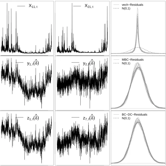
Figure 1 shows two time series plots of each, the raw series Xt, the MBC-transformed yt(ˆδ) (with semiparametric estimates ˆδj and m= 42) and the BC-DC transformedzt(ˆδ) (with univariate semiparametric estimates ˆδj andm= 3) in the left two panels. While large positive outliers occur and volatility strongly co-moves with the level of the untransformed variances and covariances, the distribution of the transformed series is more stable and symmetric around their persistent movements. Interestingly, the dynamics of the first diagonal entry of the
MBC series, y1,t(ˆδ), are very similar to the univariate transformed variancez1,t(ˆδ), while the nondiagonal MBC entry y2,t(ˆδ) evolves in close parallel to the corresponding z-transformed correlation z7,t(ˆδ). This reflects the finding of Gribisch (2013, p.4) who found and discussed the closeness of the matrix logarithm’s diagonal and off-diagonal elements to log variances and correlations, respectively.
We assess the in-sample success of various nonlinear transforms for our dataset. The ap- propriateness of a transform for modeling purposes can be seen by a parsimonious ARMA representation for the transformed variable. Additionally, the stabilization of conditional vari- ances, i.e. the conditional homoscedasticity of the residuals, is an important goal of the trans- formation. Further, the approximate normality of transformed variable or model residuals are frequently stated as the motivation for a transformation-based approach. To evaluate these goals, diagnostic residual tests are carried out for our benchmark VARMA(2,1) speci- fication which is applied to different transforms. As straightforward and familiar choices, we use univariate Ljung-Box tests both on raw residuals and on squared residuals to check serial correlation and conditional heteroscedasticity, respectively, while Jarque-Bera tests are used to detect deviations from normality. In our comparison, we consider the raw realized variances and covariances (vech), the nonzero terms of the Cholesky factors (chol) as well as the unique terms of the symmetric matrix square-root (sym-root), of the matrix logarithm (mlog) and of the inverse covariance matrices (inverse).
The results of these diagnostic tests, more precisely the number of rejections across series for different significance levels, is given in Table 3. Transformations of the realized covariance matrices which are not appropriate may be detectable by the failure of linear time series models to produce serially uncorrelated residuals. Therefore, consider the test for residual autocorrelation, given in the upper panel. Both the MBC-RCov and the BC-DC models have a non-negligible fraction of rejections. There remains significant autocorrelation even at the 0.1% level for one of the 21 series. Autocorrelation is modest compared to some of the other transformations, e.g., the Cholesky factorization, however. For the latter, the p-values are smaller than 1% in 9 cases and the majority (14 out of 21) of the residual series exert significant autocorrelation at the 5% level. The matrix logarithm transform is the hardest competitor but still exceeds the BC-DC model with respect to the number of rejections (4 versus 2 at the 1% level). A better fit of the models could be obtained by using larger VARMA model orders
globally, or by specifying the ARMA models individually for each series. We have consistently chosen an intuitive and sparse specification to enhance comparability with other model classes in light of the out-of-sample forecasting study carried out below.
Compared to the other transforms and special cases, the BC-DC and even more the MBC- RCov model (2 and 1 rejection, respectively, at the 1% level) succeed in stabilizing the residual variance. Except for the mlog-transform, all other models suffer from extreme conditional heteroscedasticity with very high rejection rates when autocorrelation of the squared residuals is tested.
Normality of the model residuals is frequently rejected for the Box-Cox specifications, namely 10 times out of 21 at the 1% level. It thus performs worse than the matrix logarithm.
Given that the matrix logarithm is contained in the family of MBC-transforms it turns out that when choosing the transformation parameters for our dataset, we face a tradeoff between obtaining linear time series models, stabilizing variance and yielding normally distributed vari- ables. The estimatedδj <0 thus prioritize the former goals but fail with respect to the latter.
Still, the normal approximation is strongly improved compared to the raw variance and co- variance series. Kernel density plots of the model residuals in the right panel of Figure 1 show the approximate normality of the transformed series as compared to the untransformed ones.
6 Forecast comparison
We assess the forecast performance of the MBC-RCov and the BC-DC models, also in light of popular competitor methods. To this end, we use the data set introduced in section 5 and conduct a quasi out-of-sample forecast exercise, recursively using a pre-specified window of data for parameter estimation and forecasting, and then, subsequently, evaluating the forecasts against realized data outside that range.
We address the following questions in the forecasting exercise. To take a closer look at the methods introduced in section 4.1, we first assess whether bias-correction leads to a significant improvement of the forecasts. Further, for both the MBC-RCov and the BC-DC model, we evaluate which value of the transformation parameter δ dominates in terms of out-of-sample precision and whether the estimates presented in section 5 are also superior out of sample. We are also interested in whether the dynamic correlation specification outperforms the matrix transform or vice versa.
Another main objective of the study is to assess the value of the transformation-based approach as compared to other methods. As a recently suggested and popular competitor we consider the class of models that assume conditionally Wishart distributed realized co- variance matrices. More specifically, two models are included in our baseline comparison, the Conditional Autoregressive Wishart (CAW) model of Golosnoy et al. (2012) and the Condi- tional Autoregressive Wishart Dynamic Conditional Correlation (CAW-DCC) specification of Bauwens et al. (2012).
6.1 Models and setup
To tackle the questions above, we apply the baseline diagonal VARMA(2,1) specification for the MBC-RCov and BC-DC model and apply a grid of fixed values for the transformation parame- ter which seem relevant for a specific comparison, e.g.,δ1=. . .=δk∈ {−0.1,−0.05,0,0.5,1}.
The other model parameters are re-estimated for each estimation window.
For the Wishart models used as benchmarks, the distributional assumption is
Xt|It−1∼Wn(ν, St/ν), (19)
where Wn denotes the central Wishart density, ν is the scalar degrees of freedom parameter andSt/ν is a (k×k) positive definite scale matrix, which is related to the conditional mean of Xt by E[Xt|It−1] =St. The baseline CAW(p,q) model of Golosnoy et al. (2012) specifies the conditional mean as
St=CC0+
p
X
j=1
BjSt−jB0j+
q
X
j=1
AjXt−jA0j, (20)
C, Bj and Aj denoting (k×k) parameter matrices, while the CAW-DCC model of Bauwens et al. (2012) employs a decomposition
St=HtPtHt0, (21)
whereHt is diagonal andPt is a well-defined correlation matrix. As a sparse and simple DCC benchmark we apply univariate realized GARCH(pv,qv) specifications for the realized variances
Hii,t2 =ci+
pv
X
j=1
bvi,jHii,t−j2 +
qv
X
j=1
avi,jXii,t−j, (22)
along with the ‘scalar Re-DCC’ model (Bauwens et al.; 2012) for the realized correlation matrix Rt,
Pt= ¯P +
pc
X
j=1
bcjPt−j+
qc
X
j=1
acjRt−j. (23)
The diagonal CAW(p,q) and the CAW-DCC(p,q) specification with p = pv = pc = 2 and q=qv =qc= 1 are selected since they are similar in complexity to the diagonal VARMA(2,1) model and provide a reasonable in-sample fit among various order choices.
For a given forecasting method, the evaluation is carried out as follows: We split the avail- able data in a sampleX1, . . . , X1508 which is used only for estimation and an evaluation sample X1509, . . . , X2156. For eachT0 ∈[1508; 2156−h], the model is estimated using a rolling sample XT0−1507, . . . , XT0 of 1508 observations and forecasts ofXT0+h,h= 1,5,10,20, are computed.
For the transformation-based forecasts, we consider both the na¨ıve forecastXeT0+h|T0, based on (14), and the bias-corrected forecastXbT0+h|T0, see (15), usingR= 1000 simulated realizations.
In addition, density forecasts of the returns rT0+h given IT0 are computed using the same simulated trajectories as for the bias-corrected covariance forecasts.
As outlined in section 4.1, in the simulations we discard trajectories where the transfor- mation from yt(i) to Xt(i) is not well-defined. Additionally, to attenuate the effect of extreme outliers in the simulated paths, we replace an element of the bias-corrected covariance matrix forecast by the uncorrected forecast if the fraction between the two exceeds 5 in absolute value.
Such a procedure reflects a practically feasible plausibility check. Both modifications of the forecasts are needed only for small values of the transformation parameters δ ≤ −0.25 in our study which are anyway inconsistent with the empirical interval estimates presented above.
We compare the forecasting models by presenting average losses, i.e. risks, over the evalua- tion period. To gain insights about statistical significance of the differences, model confidence sets (MCS) are constructed following Hansen et al. (2011) using the MulCom package (Hansen and Lunde; 2010) in Ox Console Version 6.21. The Max-t statistic is bootstrapped with a block lengths ofd= max{5, h}and 10000 iterations. A confidence level of 90% is used throughout.
6.2 Baseline results
We begin with an evaluation of the forecasting performance using a simplesquared prediction error loss function, evaluated using the true realized covariance matrices. For h = 1,5,10,20 andT0 = 1508, . . . ,2156−h, we compute the period loss as the Frobenius norm of the forecast
error
LFT{s}0,h=
k
X
i=1 k
X
j=1
Xij,T0+h−Xij,T{s}0+h|T0
2
, (24)
whereXT{s}0+h|T0 is a covariance matrix forecast obtained from one of the different methods.
To assess the value of the bias-correction we compare the risk LF{s}h = 1
2156−h−1507
2156−h
X
T0=1508
LFT{s}0,h
of the corrected forecasts to the na¨ıve ones by calculating the fraction of the two for the different models and transformation parameters. The results are given in Table 4. Despite the adjustment of miss-behaved bias-corrected forecasts outlined in section 6.1, the simulation- based forecasts are worse than the uncorrected ones forδ ≤ −0.25. This is most pronounced for the MBC-RCov model and for short horizons. In such cases, the normality assumption provides a poor description of the transformed variables and hence the simulatedyt(i) series do not produce well-behaved re-transformed forecasts.
The valuation of bias correction changes fundamentally whenδ≥ −0.1 is considered. This is the empirically relevant span as the estimates of section 5 suggest. The simulation-based procedure leads to marked improvements of the forecasts. The reduction in risks for the MBC- RCov model is as high as 12% forh = 1 and δ =−0.1; it gradually reduces as δ approaches one. There, the MBC-transform corresponds to the raw covariance series and bias-correction is not needed. This broad picture is reflected also by the BC-DC transformed series, where δ= 0.5, corresponding to a model of realized standard deviations, is minimally prone to bias.
Forδ = 1, when untransformed realized variances are approximated by a Gaussian process in the simulations, the latter fail to reduce bias, and even devastate the forecast accuracy.
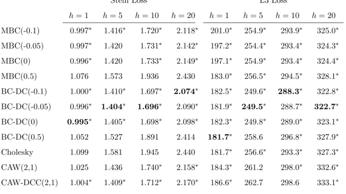
Having shown the usefulness of bias correction, we now turn to a comparison of bias- corrected forecasts of the proposed models along with the CAW and CAW-DCC specification for which a correction is not needed. The corresponding Frobenius risks are shown in the left part of Table 5. The boldface numbers, which indicate the best-performing model for each horizon, show that the BC-DC specification withδ ∈ {−0.1,−0.05} emerges as favorable for all horizons.
The asterisks indicate models contained in the 90% model confidence set for a given horizon h. The MBC-RCov forecasts are contained only for a few specific values of δ. For one-step forecasts, only the matrix square root transformed (δ = 0.5) and untransformed (δ = 1)
forecasts cannot be rejected. For some other horizons, no MBC-RCov specification (h= 5) or only those with negative δ (h = 20) resist a rejection. Neither the matrix logarithm (δ = 0) nor the semiparametric estimates ofδ provide a reasonable performance which is robust with respect to the chosen horizon. The BC-DC model forecasts are elements of the MCS for a wide range of transformation parameters including the estimates from section 5 as well as δ = 0.
This holds for all considered forecast horizons. A comparison to the Wishart models reveals that despite their larger risk, both models cannot be rejected by the MCS approach except for the two-weeks horizonh= 10.
These conclusions about superiority change when the density forecasts are considered. We evaluate the forecasts by the logarithmic scoring rule; see, e.g., Gneiting et al. (2008),
LD{s}T0,h=−logfr{s}(rT0+h|IT0), (25) computing negative logarithms of the density forecast fr{s}, evaluated at the realized daily returns h periods ahead. The logarithmic rule is a strictly proper scoring rule, rewarding careful and honest assessments (Gneiting and Raftery; 2007). It is local in the sense that no point of fr{s} other than the realized return is evaluated, which is also an intuitively and computationally appealing property.
The results are given in the right part of Table 5. Here, the MBC-RCov with δ ≈ 0 outperforms the BC-DC model; significantly forh = 1 as the MCS consists of only one spec- ification there. For larger horizons, the differences are less pronounced and both models with transformation parameters close to zero seem appropriate.
To understand this outcome, note that the whole density of XT0+h given XT0 is involved in computing the conditional return density forecasts. The matrix logarithmic model stands out from its competitors in yielding relatively close-to-Gaussian residuals, as has been seen in section 3. Since we use the truncated normal distribution in our simulation ofXT(i)0+h, the different model rankings with respect to covariance forecasts and return density forecasts can be understood in light of this finding.
Also the Wishart models are rejected using the log density metric. We regard this as evidence that the Gaussianity assumption for transformed realized covariances provides a better approximation than the Wishart specification — at least when it comes to forecasting the return distribution.
To conclude the baseline results, the BC-DC model with small negative δ outperforms in terms of covariance matrix forecasting, while the MBC-RCov model withδ ≈0 emerges when the aim is forecasting the return density. The Wishart models are outperformed significantly in the latter case.
6.3 Robustness regarding model specification
Up to now, the results for MBC-RCov and BC-DC forecasts are based on a simple diago- nal VARMA(2,1) specification. We check whether our conclusions with regard to the data transformations remain intact for other models which have been used for volatility dynamics.
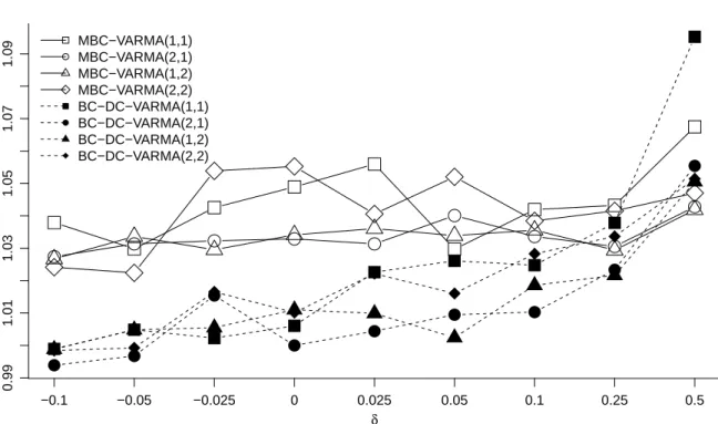
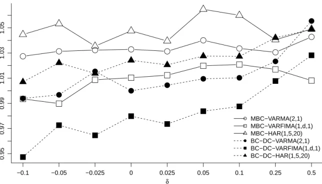
We first assess whether the choice of VARMA order matters for our conclusion. To this end, we compute forecasts and risks also for other specifications. The result for the Frobenius loss and h = 10 is exemplarily shown in Figure 2 and mirrors the result for other horizons.
To make the figures comparable, here and henceforth, the risks are plotted as a fraction of a common benchmark, the BC-DC model with VARMA(2,1) dynamics and δ = 0. It turns out that the VARMA(2,1) specification is among the best choices for most of the different transformation parameters. Importantly, the conclusion about favorable transforms does not interfere with the choice of model orders.
Daily financial volatility is often associated with a long memory behaviour, so we also include such models to our robustness checks. As a first alternative, we consider the heteroge- neous autoregressive model of Corsi (2009). Lags of yit(δ), averaged over 1, 5 and 20 trading days in the process
yit(δ) =ci+αi1yi,t−1(δ) +αi5
1 5
5
X
j=1
yi,t−j(δ)
+αi20
1 20
20
X
j=1
yi,t−j(δ)
+uit (26) introduce long-memory-like persistence. The parameters are estimated by least squares. In contrast, Chiriac and Voev (2011) use a flexible fractionally integrated vector ARMA (VARFIMA) specification with “real” long memory behavior. We also follow their approach but do not re- strict the memory parameter to be the same across series, and hence estimate series-specific parametersθi = (di, αi1, . . . , αip, φi1, . . . , φiq, µi) of
(1−αi1L−. . .−αipLp)(1−L)di(yit(δ)−µi) = (1 +φi1L+. . .+φiqLq)uit. (27) Again, correlation between the series is introduced only through the noise covariance matrix
Σu. Like Chiriac and Voev (2011) we setp=q = 1 which gives the same model complexity as in our benchmark VARMA(2,1).
Overall, the VARFIMA setup provides smaller forecast errors than the VARMA bench- mark, while the HAR is outperformed by both competitors; see the results in Figure 3. The excellent results for the ARFIMA model are in line with the results of Chiriac and Voev (2011).
Further gains may be attainable by considering more sophisticated models, e.g., taking possible dynamic spillovers, factor structures and structural breaks into account. While a comprehen- sive comparison of different dynamic specifications is beyond the scope of this paper, we direct attention to the relative benefits of the various transformations for a given model. The relative rankings remain remarkably unchanged, independently of the dynamic specification. Again, the BC-DC model with small negativeδj stands out.
Lastly, we compare our transformation-based approach to other models of the conditional Wishart family. To this end, we conduct a comparison of several diagonal CAW(p,q) models and CAW-DCC(p,q) models with different orders p and q. Additionally, the component mod- els proposed by Jin and Maheu (2013) are considered. Regarding the latter, we estimate a Wishart Additive Component (CAW-ACOMP) model. The distributional assumption (19) is complemented by
St=CC0+
K
X
j=1
BjΓt,lj, Bj =bjb0j, Γt,l= 1 l
l−1
X
i=0
Xt−i, (28)
where denotes the elementwise (Hadamard) product and, analogously to the HAR model, past averages of the covariances enter the conditional mean equation in a linear manner.
Similarly, such lower frequency components are also involved in the Wishart Multiplicative Component (CAW-MCOMP) model
St=
1
Y
j=K
Γ
γj 2
t,lj
CC0
K
Y
j=1
Γ
γj 2
t,lj
, (29) which we also assess in our study. As for the HAR model, we set K = 3 and average over l1 = 1, l2 = 5 and l3 = 20 past observations. In accordance with all other Wishart models considered so far, the parameters are estimated by maximum likelihood for all rolling samples.
The results which are shown in Figure 4 for the Frobenius loss are clear-cut. None of the models outperforms the BC-DC benchmark, irrespective of the forecasting horizon. This is indicated by the relative risks that are above one for all models. In contrast, the ranking
among the Wishart models varies with the horizon. At least for the smaller horizons, the chosen benchmark orders p = 2 and q = 1 correspond to well-performing models. The component models show an ambiguous figure. The additive model does well for most horizons, but the multiplicative approach is worthwhile only for rather long-term forecasts (h= 20).
Overall, the robustness checks find that the results of the baseline setup remain qualitatively unchanged also when other dynamic models, both for the Box-Cox models and for the Wishart family, are taken into account. Among the considered alternatives, long memory BC-DC models are the most relevant direction for improvements.
6.4 Robustness regarding loss function
So far we have focussed on the Frobenius norm of the forecast error when evaluating the covariance matrix forecasts. In the matrix case, there are several other loss functions which may be appropriate for different practical forecasting situations; see, e.g., Laurent et al. (2013) for a discussion. In our out-of-sample study, we additionally consider the Stein distance
LST0,h= trh
XT−10+h|T0XT0+hi
−log
XT−10+h|T0XT0+h
−k, (30) and the asymmetric loss
L3T0,h= 1 6trh
XT30+h|T0−XT30+h
i− 1 2trh
XT20+h|T0(XT0+h−XT0+h|T0)i
, (31)
which is used by Laurent et al. (2011). Forecast comparisons based on LF, LS and L3 may differ becauseLS penalizes underpredictions more heavily thanLF while overpredictions are more influential with theL3 loss, see Laurent et al. (2011), section 2.3. Additionally, the loss functions differ in their relative importance of high versus low volatility periods since only the Stein distance is homogeneous of order 0 and hence scale invariant.
The results of the evaluation with the Frobenius norm is replicated using both the LS and the L3 norms. Again, as Table 6 reveals, the BC-DC models perform better than their MBC-RCov counterparts and their forecasting superiority is not rejected with zero or small negative transformation parameter. The CAW models are statistically rejected in some cases, even if the power of the MCS procedure appears small for the L3 loss.
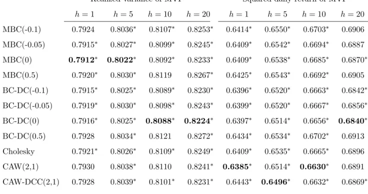
A reasonable loss function may also be chosen to involve the economic cost of prediction errors. A risk-averse investor may be interested in the variance of an ex-ante minimum-variance
portfolio (MVP) which is computed from the covariance matrix forecast. Using the realized variance of the MVP as the ex-post loss, we therefore consider
LM VT0,h=w0XT0+hw, where w= (ι0XT0+h|T0ι)−1XT0+h|T0ι, (32) where ι = (1, . . . ,1)0. Alternatively, the squared daily return w0rT0+hr0T0+hw of the ex-ante MVP is used instead of the realized variance.
Table 7 shows rather inconclusive results. The discriminating power is weak for these two losses, so that many models are included in the model confidence sets. Notably, however, BC-DC withδ = 0 outperforms in three out of eight horizon-loss combinations and is always included in the MCS.
To summarize, the forecasting results are unchanged if other dynamic models are considered and reveal relatively little ambiguity also with alternative loss functions. Overall, the Box-Cox dynamic correlation specification with log variances (δ = 0) seems to be a good and robust choice in practice. It is close to the best performing model for most horizons and with regard to many of the evaluation criteria. The MBC-RCov model, however, has a superior forecasting performance for specific criteria such as predictive densities. Further research appears fruitful to further clarify these facts, e.g., in light of datasets for different asset classes.
7 Conclusion
We have proposed two new approaches to multivariate realized volatility modeling and applied them to US stock market data. The empirical results, including an out-of-sample forecasting comparison, seem promising, also in comparison to the main competitors, the conditional autoregressive Wishart model of Golosnoy et al. (2012) and several variants thereof. Our assessment of various transformation parameters supports a convenient special case of our Box-Cox approaches: the use of standard linear time series models to a multivariate time series of log realized variances and z-transformed correlations. Its appropriateness can be easily checked for a specific dataset using the inferential methods introduced in this paper.
The present study leaves significant questions for further research. With a focus on forecast- ing, investigating more advanced dynamic specifications appears worthwhile, possibly including dynamic spillovers and structural changes along with the long memory dynamics briefly consid- ered in this paper. Additionally, in applications to data sets of higher dimensions, our approach
allows the assessment of cross-sectional properties such as factor structures in a methodolog- ically and computationally straightforward setup. In addition to the realized volatility setup with utilization of intraday data, our models are also relevant for the study of multivariate stochastic volatility based on a latent covariance matrix specification.