Regensburger
DISKUSSIONSBEITRÄGE zur Wirtschaftswissenschaft
University of Regensburg Working Papers in Business, Economics and Management Information Systems
Capturing the Interaction of Trend, Cycle, Expectations and Risk Premia in the US Term Structure
Max Soloschenko*, Enzo Weber**
April 22, 2014 Nr. 475
JEL Classification: C32, C58, E43, G12
Keywords: unobserved components, expectation hypothesis, cointegration, identification, risk premium
* University of Regensburg, Department of Economics and Econometrics, 93040 Regensburg, Germany.
max_soloschenko@web.de.
** University of Regensburg, Department of Economics and Econometrics, 93040 Regensburg, Germany.
enzo.weber@wiwi.uni-regensburg.de, phone: +49 941 943 1952, and Institute for Employment Research (IAB), IOS Regensburg.
Capturing the Interaction of Trend, Cycle, Expectations and Risk Premia in the US Term Structure
Max Soloschenko* Enzo Weber†
ABSTRACT
This paper deals with simultaneous interactions between the determinants of the US yield curve. For this purpose, we derive a multivariate unobserved components model based on the expectation hypothesis. The influencing factors of the term structure that arise from the structural model are a common stochastic trend, the cyclical part of the short rate and maturity-dependent term premiums in the longer rates. We establish a significant influence of both permanent and transitory innovations on the US term structure and find pronounced spillovers between the shocks of the term structure determinants. An interesting result depicts a key role of the spillovers of structural mid-term rate cycle shocks in the formation of the risk premiums.
JEL codes: C32, C58, E43, G12,
Keywords: unobserved components, expectation hypothesis, cointegration, identification, risk premium.
* University of Regensburg (E-mail: max_soloschenko@web.de)
† University of Regensburg, IOS Regensburg and Institute for Employment Research (IAB) (E-mail: enzo.weber@wiwi.uni-regensburg.de)
INTRODUCTION 1
1 INTRODUCTION
There exists a broad range of theories and empirical models designed to analyse the term structure of interest rates. These make use of a multitude of observed and unobserved factors that may influence the term structure – such as risk premiums, inflation expectations and monetary policy. The interactions between these influencing factors have, however, received little attention in the relevant literature. Nevertheless, for both policy makers and market participants, knowledge about such interactions can provide valuable insights into market mechanisms.
We specify a multivariate model of the US yield curve, consisting of 1-month, 3-year and 10- year interest rates, which covers the short-, mid-, and long-term horizons. This framework focuses on capturing the simultaneous causality structure between the components of the term structure model – trend, cycle, expectations of future short rates and risk premiums. Within this framework we can measure whether the determining factors are affected purely by their own innovations or if spillovers also play a significant role. Moreover, due to the flexible specification of the structural model, it will be possible to test the coefficient restrictions implied by the expectation hypothesis of the term structure (EHT).
In order to analyse the US yield curve, this paper combines theoretical and empirical frameworks. The EHT serves as a starting point, representing long-term rates as an average of the expected future short-term rates. Further, we combine the EHT with time-varying risk premiums. From an econometric point of view, we decompose the short rate into a permanent and a transitory unobserved component (UC). Then, using this stochastic short rate specification, we derive the processes for the longer-maturity rates. The influencing factors of the term structure that arise from the structural model are a common stochastic trend, the transitory or cyclical part of the short rate and maturity-dependent term premiums in the longer rates. The first component determines the level of the yield curve, meaning that trend shocks shift all interest rates. The second factor, the cyclical component of the short rate, captures the individual alignment of the interest rates or the slope of the yield curve. The same applies to the risk premium components affecting the longer-maturity rates. The term premium components denote the horizon-specific compensation for the risks related to an investment in longer-maturity bonds (cf. Gürkaynak and Wright 2012). These interpretations link the first two components to the “level” and “slope” factors known from affine term
INTRODUCTION 2 structure models (cf. Duffie and Kan 1996, Dai and Singleton 2000, Duffee 2002 amongst others). In contrast to this literature, our framework explicitly aims to decompose interest rates into trend and cycle components. Thus, in this paper, the determinants of the short- and long-term yields merge into a multivariate simultaneous UC model with cointegration;
compare also Schleicher (2003), Morley (2007) or Sinclair (2009). Our analysis focuses on capturing the simultaneous interactions between the innovations of the term structure components. For this purpose, we decompose the errors of the UCs in such a way that each can be influenced by both its own structural shocks and those of the other factors. As a consequence, each determinant is allowed to be hit at the same time by structural trend as well as cycle shocks. Moreover, the model framework has been extended by volatility regimes in order to take into account the heteroscedasticity and also to strengthen identification of the model (cf. Sentana and Fiorentini 2001, Rigobon 2003, Weber 2011).
The results suggest that both types of shocks, permanent and transitory, have considerable influence on the US term structure. We also establish strong spillovers between the yield curve determinants. A prime example is the structural shock to the mid-term rate cycle, the spillovers of which affect the cycle component of the short rate noticeably and play a key role in the formation of the risk premiums. This can be explained by the fact that the uncertainties contained in the mid-term rate are also immediately relevant for the longer horizon.
Moreover, we find that the structural short rate cycle shock – which can be related to the influence of monetary policy – affects the short rate through both a permanent and a transitory channel, although its effect is more pronounced on the short end of the yield curve. The trend component (or level factor) is affected by its own structural shock and the aforementioned spillover of the structural short rate cycle shock. Thus, the risk premia have no effect on the level of the term structure. In our analysis, we apply a generalised model, which does not impose a priori restrictions from EHT on the coefficients. Indeed, we find that empirically, these restrictions cannot be confirmed.
The paper is organised as follows: it begins with a structural UC model of cointegration based on the EHT. Here the identification issues are also addressed in greater detail. The specification and empirical application of the structural framework is presented in the subsequent section, which deals additionally with the interpretation of the outcomes and discusses some potential macroeconomic implications arising from the structural model. The final section summarises the analysis and provides promising directions for future research.
THE MODEL 3
2 THE MODEL
2.1 MODEL DEVELOPMENT
We start with the pure EHT which states that under the no-arbitrage condition a single n- period fixed-interest investment should yield the same return as a series of n successive one- period investments. Further, we extended the framework by maturity-dependent time-varying risk premiums ct(n), which express agents' risk aversion. In linearised form the EHT can be written as
) ( 1
0 )
( 1 n
t n
i
i t t n
t Er c
R n
, (1)
where Rt(n) denotes the interest rate of maturity n1 and rt of maturity one (n1). Thus, the long-term rate equals the average of the future expected one-period interest rates (forward rates). The operator Et expresses rational expectations given all available information at a time t. The risk premium ct(n) is assumed to follow an AR(p) process: (n)(L)ct(n) t(n). This time-varying specification can capture both cases, stationary and non-stationary term premia. Since the present specification implies Et(ct(n))0, the equations for the long-term rates will be later extended by a maturity-specific constant in order to capture the mean of the respective risk premium.
The process for the short-term (one-period) rate rt is represented as the sum of two unobservable components: a stochastic trend t and a cyclical component ct(1) (see e.g. Stock and Watson 1988):
) 1 ( t t
t c
r
. (2)The individual components are specified as follows:
t t
t
1 , t ~N(0,2), (3)) 1 ( ) 1 ( ) 1
( (L)ct t
, t(1) ~N(0,2(1)). (4)
THE MODEL 4 Thus, the trend follows a random walk and the transitory part is an AR(2) process.1 In modulus, all roots of the lag polynomial (1)(L)11(1)L2(1)L2 lie outside the unit circle.
The linkages of the shocks to the unobserved components will be treated below.
Based on the EHT and the stochastic specification for the short rate we can derive the processes for the long rates Rt(n). These are obtained by substituting equations (2) through (4) into (1), applying the expectations operator and rearranging terms. For the first three yields this can be illustrated as follows:
) 2 ( ) 1 (
1 ) 1 ( ) 2 1 ( ) 1 ( ) 1
2 ( ) 2 ( 1 )
2 (
2 2
) 1 2(
1
t t t
t t
t t t
t r Er c c c c
R ,
) 3 ( ) 1 (
1 ) 1 ( 2 ) 1 ( 1 ) 1 ( ) 2 1 ( ) 1 ( 2 )2 1 ( 1 ) 1 ( ) 1
3 ( ) 3 ( 2 1
) 3 (
3 3
) 1 3(
1
t t t
t t
t t t t t
t r Er Er c c c c
R ,
2(1) 1(1) 2(1) (1)
)3 1 ( 1 )2 1 ( 1 ) 1 ( ) 1
4 ( ) 4 ( 3 2
1 )
4 (
4
2 ) 1
4( 1
t t
t t t t t t t t
t r Er Er Er c c
R
(11) (4)
) 1 ( 2 )2 1 ( 1 ) 1 ( 2 ) 1 ( 1 )2 1 ( 2 ) 1 ( 2
4 ct ct
, (5)
where (n)denotes a maturity specific constant. From (5) it is clear that the coefficients of ct(1) and ct(1)1 are the functions of the AR polynomial from (4) and the maturity n, which leads to the general form:
) ( ) 1 (
1 ) 1 ( 2 ) 1 ( 1 ) 1 ( ) 1 ( 2 ) 1 ( 1 )
( )
(n n t ( , , ) t ( , , ) t tn
t f n c g n c c
R , (6)
where the functions f(.) and g(.) denote factor loadings. Moreover, similar to Startz and Tsang (2010), for real roots the factor loadings can be expressed as functions of the roots of the characteristic equation shown in (4):
(1)
2 2 2
1 1 1
2 1 )
( ) (
) ( 1
) 1 ( 1 )
1 ( 1 1
t n n
t n n
t c
n R n
n
1 The empirical suitability of the AR order of two will be verified.
THE MODEL 5
) ( ) 1 (
1 1 1 2
2 2
1 2 1
) ( 2
) 1 ( 1 )
1 (
1 n
t t n n
c n c
n
n
.
(7)
where i(n), i1,2, denotes the effect of the short-term cycle component on the long-term rate. Thus, the EHT has the following implications for the unobserved components: firstly, the trend component influences all yields with the same strength (i.e., one), regardless of their maturity. It reflects the fact that shocks to a component that is permanent are expected to remain in all future short rates and, thus, also in their mean from (1). Consequently, t shifts all interest rates parallel upwards or downwards and can thus be identified as a level factor.
Secondly, since each shock on the rt cycle is transitory, its impact on the average of the short rates decays with rising n. This implies declining values of i(n). Logically, the cycle can be seen as a slope factor. This interpretation is in line with the affine term structure literature e.g.
Duffie and Kan (1996), Duffee (2002), Kim and Orphanides (2005), Kim and Wright (2005), Diebold and Li (2006).
For the empirical analysis of the term structure we specify a trivariate system, which contains a medium-term (36 months) and a long-term (120 months) yield besides the 1-month rate:
The structural framework from (8) through (10) denotes a generalised version of the theoretical model from (7). This representation enables to avoid any parametric restrictions from the outset and allows the data to determine the respective contributions of trend and cycle. For the trend this is achieved by introducing and .2 These coefficients measure the fraction of the common permanent component in the respective long-term rates, which will equal one in the case of the EHT. Moreover, from the outset we set no EHT restrictions on the four (n)s.
2 For the empirical analysis the permanent component will be extended to random walk with drift, since the data reveals clear trend behaviour within the selected time period.
) 1 ( )
1 (
t t
t c
r
, (8)) 36 ( ) 1 (
1 ) 36 ( 2 ) 1 ( ) 36 ( 1 )
36 ( ) 36 (
t t t
t
t c c c
R
, (9)) 120 ( ) 1 (
1 ) 120 ( 2 ) 1 ( ) 120 ( 1 )
120 ( ) 120 (
t t t
t
t c c c
R
. (10)THE MODEL 6 The major innovation of the current paper lies in its examination of the interactions between the determining factors of the term structure. In the present model, these factors are the trend, short rate cycle and the maturity-specific, time-variable term premiums. We introduce a novel structure that captures the simultaneous interactions between the unobserved components. This extension decomposes the shocks t, t(1),t(36) and t(120) into structural innovations, compare also Weber (2011):
Thus, the components innovations from t are the composites of the structural innovations (henceforth: composite shocks). ~ , t ~t(1), ~t(36)and ~t(120)from the vector ~ denote structural t uncorrelated shocks of the common trend and three cycles (henceforth: structural shocks).
This structure allows for correlation between the components and at the same time decomposes the interaction between them. Accordingly, the common trend and the three cycles can be hit by trend- as well as cycle-specific shocks. The off-diagonal elements are spillover coefficients and describe the simultaneous interaction between the four unobserved components, t, ct(1), ct(36)and ct(120). The coefficients of the components-specific shocks are normalised by kii 0, i1,2,3,4.
As will be shown below in Figure 1, the data under consideration include a high volatility regime in the period from late 1979 to late 1982, commonly related to the Volcker period.
This is also in line with the variance break point suggested by Startz and Tsang (2010) or Weber and Wolters (2013). Moreover, since the subprime crisis led to an historically low interest rate level, it would be appropriate to verify a potential change in the variance level for this period. We capture heteroscedasticity as follows: our approach considers several regimes (with different volatilities) for the data generating process of the structural shocks from (11).
The structural variances of (say) the first regime are normalised to 1: Var(~t |tQ1). Qq denotes a set of time points that belongs to the qth regime (where q1,...,s) and s indicates the number of volatility regimes. The variances of further regimes (Var(~t|tQl), where
t t
t t
t t
K t
t t
t
k k k k
k k k k
k k k k
k k k k
~ ) 120 (
) 36 (
) 1 (
44 43 42 41
34 33 32 31
24 23 22 21
14 13 12 11
) 120 (
) 36 (
) 1 (
~
~
~
~
. (11)
THE MODEL 7
s
l 2,..., ) are parameters that need to be estimated. Should variance break(s) have indeed taken place, at least some values will be significantly different from one.
2.2 REDUCED FORM AND IDENTIFICATION
For the model to be identified, enough information must be extracted from the reduced form in order to recover the structural parameters. The reduced form of the structural model is deduced by substituting the specifications of the respective unobserved components into equations (8) through (10), taking first differences or solving for cointegrating relationships and rearranging terms. One obtains the vector autoregressive integrated moving average (VARIMA) representation given in (12).3 Then, this structural model VARIMA must be matched with its reduced form VARIMA representation (13) given by virtue of Granger's lemma (Granger and Newbold 1977):4
) (
) (
) ( ) ( 0
0 0
0
0 )
( ) ( 0
0 0
0 0
) ( ) ( 0
0
0 0
0 )
( ) ( 0
0 0
0 0
) (
) 1 ( ) 120 (
) 1 ( ) 36 (
) 120 (
) 36 (
) 1 (
120 1
36 1 120
1 36
1 1
t t
t t
t t t
r R
r R
R R r
L L
L L L
L L
L L
3 For simplicity we set (n)0 in the formal derivation.
4 For more on identification of the correlated multivariate UC models see Schleicher (2003), Morley (2007), Sinclair (2009) and Soloschenko and Weber (2013).
(1)1120 ) 120 ( 2
36 ) 36 ( 2
120 ) 120 ( 2
36 ) 36 ( 2
) 120 (
) 36 (
) 1 (
1 120
) 120 ( 1
1 36
) 36 ( 1
1 120
) 120 ( 1
1 36
) 36 ( 1 120
1 36 1
1
) (
) (
) (
) ( 0
) ( 0
) ( ) (
0 ) ( ) ( ) (
) ( 0
) (
0 ) ( )
(
0 0
0 0
) ( ) (
) ( ) (
) (
t
t t t t
L L L L
L L
L L
L L
L L
L L
L L
L
, (12)
(120)
) 36 (
) 1 (
53 52
51
43 42
41
33 32
31
23 22
21
13 12
11
) ( )
( )
(
) ( )
( )
(
) ( )
( )
(
) ( )
( )
(
) ( )
( )
(
t t t
L L
L
L L
L
L L
L
L L
L
L L
L
. (13)
EMPIRICAL PART 8
The reduced form innovations t(j) consist of the composite shocks in (12), which are linear combinations of the structural shocks. For p2, the structural model leads to a VARIMA(4,1,4) process. The coefficient matrix from (13) is a matrix-polynomial, which consists of individual MA lag polynomials (L) and (L); the latter result as linear combinations of the former (cf. Morley 2007, Soloschenko and Weber 2013). The polynomials dk(L) are normalised by setting the first element to one if d k and zero if
k
d , where d,k1,2,3.
The last two rows identify the common trend coefficients and . The AR coefficients of the three cyclical components i(j) (where j1,36,120 and i1,2) are directly identified by the autoregressive parameters from (13). Thus, in the two regime case, there are a further 24 parameters to be identified – the 16 spillover coefficients from the K-matrix, four (n) coefficients and the four structural variances of the second regime, or in general 204
s1
. As mentioned above, in order to capture heteroscedasticity we specify the variance breaks from the outset. Consequently, each further regime increases the number of unknown coefficients by four per break. On the other hand, additional identifying autocovariance equations from the MA part of (13) are provided for all s regimes separately. Then, in order to check identification of the structural model, one has to equate autocovariance functions of the right-hand side of (12) and (13): ()q and ()q, where 04, q1,2 and for4
(
)q (
)q 0. To sum up, the MA part of (13) delivers five autocovariance matrices per regime, which provide six parameters from the symmetric matrix (0)q and nine from each of the remaining four matrices. This provides s
69(2p)
determining equations to identify the coefficients from the structural model. Comparing these terms, identification requires 8s(19p). Thus, for s2 and p1 the structural model would be already (over-)identified.3 EMPIRICAL PART
3.1 DATA
Our time series consists of monthly observations of the US certificate of deposit rate (for
1
n ) and constant maturity bond yields (for n36,120) obtained from the Federal Reserve.
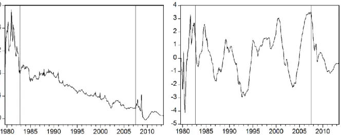
EMPIRICAL PART 9 This allows us to cover long-, mid-, and short-term horizons. Our sample starts with the beginning of Volcker's chairmanship in August 1979 and ends in June 2013. All three time series are plotted in Figure 1. The vertical lines denote the potential breaks in structural variances, which will be addressed below in greater detail:
FIG. 1: Development of the 1-month, 3-year and 10-year US interest rates.
The three time series in Figure 1 trace a similar path and display a trend pattern. At the beginning (up until the first vertical line) the data reveals strong variations, which are only moderate or low for the middle or last period, respectively. During the subprime crisis (the period from the second vertical line onwards), the short-term rate reached an historic low.
Moreover, between the end of 2008 and late 2012, the difference between the short and long- term rates rose considerably.
3.2 MODEL SPECIFICATION
The persistence of the time series is investigated by the ADF and KPSS tests, see Table 1.
Both tests confirm the presence of unit roots in the data. The ADF test clearly confirms the null of a unit root for the maturities of 1 and 36 months and only (marginally) rejects for the long rate at the 5% level. The number of cointegration relations and stochastic trends in the system is verified by Johansen trace tests. For the cointegration analysis the VAR lag length was set to two according to the Schwarz criterion. Moreover, we allowed for a constant and a linear trend in the cointegration equations. Two cointegration relations were found between
EMPIRICAL PART 10 the three interest rates, since the Johansen trace test rejects the null of no cointegration and of at most one cointegration equation at the 1% level.
n ADFa) KPSSb)
Lags of differences t-statistic 5% critical value LM-statistic 5% critical value
1 11 -2.72 -3.42 0.16 0.14
36 2 -3.26 -3.42 0.14 0.14
120 2 -3.48 -3.42 0.22 0.14
a) t-statistic is given for the null of “unit root”; Lag length determined by Modifiedc) Schwarz criterion with max. lags of 12;
all models with constant and linear trend. b) Tests the null of stationarity; KPSS bandwidth selection: Newey-West.
c) corrected for serial correlation.
TAB. 1: Unit root (ADF) and stationarity (KPSS) tests.
In the relevant literature, the end of Volcker disinflation period in the early 80s is associated with a volatility shift in the US economic and interest rate data (cf. Kim and Nelson 1999, Startz and Tsang 2010, Weber and Wolters 2013) and is also related to changes in monetary policy strategy (Thornton 2008). We set a break in the structural variances in October 1982, which is supported by the largest likelihood in a breakpoint search. As shown in Figure 1, the second potential volatility shift can be found in the period from mid-2007 onwards. Since July 2007 is often used as the beginning of the recent financial crisis, this date was selected as a potential break point. This allows for an analysis of the impact of the crisis on the term structure and its contemporaneous interactions. Moreover, the estimation of the structural model with an AR(3) specification for the unobserved cycle components could not deliver significant point estimates for the third lag coefficients. Thus, we stay with the lag length of two for the empirical analysis.
Since the data in Figure 1 reveals trend behavior, we let the permanent component follow a random walk with drift.5 In this context, note that we allow for general weights of t in (9) and (10). These weights apply both to the common stochastic trend and to the drift. Since this is potentially too restrictive for the data at hand, we integrated additional deterministic trends in (9) and (10). This generalizes the model, which still contains the original setup as a special case. The ADF, KPSS and Johansen trace tests were performed using Eviews 5 statistical software, while the structural model was estimated in GAUSS 9.
5 This has only one implication for the theoretical model shown in (5) – (7): the maturity dependent constant now also depends on the drift.
EMPIRICAL PART 11
3.3 ESTIMATION AND RESULTS
The estimated parameters from the structural model, as well as the eight respective variances of the two additional regimes, are presented in equations (14) to (22).6 Because of the potential distortion of Wald-type tests (e.g. Dufour 1997, Nelson and Startz 2007), LR tests were performed in order to verify the significance of the coefficients. The respective LR test statistics are given in parentheses.7
Term structure equations:
Components equations:
The variances of the second regime:
The variances of the third regime:
6 This output is determined through the successive elimination of the insignificant point estimates, where the omitted coefficients are individually and jointly insignificant. In this context, the insignificance of
k32 and k42 is not surprising, since the influence of the short-term cycle on the mid- and long-term rates is modelled separately.
7 The LR test statistic is chi-square distributed with 1 degree of freedom under the null. The critical values are 2.71 for the 10% level, 3.84 for the 5% level and 6.63 for the 1% level. For the four structural variances of the second and third regime the usual significance levels are unlikely to hold true in the present case, since under the null hypothesis, the variances are on the boundary of the admissible parameter space.
) 1 ( )
1 (
t t
t c
r
, (14)) 36 ( ) 1 ( ) 1 11 . 1 ( ) 1 ( ) 97 . 4 ( )
42 . 8 ( ) 32 . 14 ( ) 69 . 16 ( ) 36
( 7.542 0.018 0.339 t 0.754 t 0.217 t t
t t c c c
R , (15)
) 120 ( ) 1 ( ) 1 99 . 1 ( ) 1 ( ) 26 . 3 ( ) 62 . 4 ( ) 60 . 7 ( ) 60 . 12 ( ) 120
( 8.742 0.017 0.240 t 0.308 t 0.071 t t
t t c c c
R , (16)
t
t t
t t
t t
(120)
) ( ) 36 ( ) ( ) 1 ( ) 53 . 4 ( ) 21 . 240 1 ( ) 75 . 5 (
0 ~ 0 ~
966~ .
~ 0 074 . 1 028
.
0
, (17)
(1)
) 120 ( ) 03 . 7 ( ) 36 ( ) 99 . 23 ( ) 1 ( ) 69 . 3 ( )
05 . 6 ( ) 1 ( ) 2 07 . 66 ( ) 1 ( ) 1 17 . 70 ( ) 1
( 1.750 0.762 0.268~ 0.602~ 0.186~ 0.023~
t
t t
t t
t t
t c c
c
, (18)
(36)
) 120 ( ) 19 . 6 ( ) 36 ( ) 53 . 394 ( ) 1 ( ) ( ) 89 . 7 ( ) 36 ( ) 2 51 . 30 ( ) 36 ( ) 1 68 . 54 ( ) 36
( 1.226 0.310 0.258~ 0~ 0.448~ 0.037~
t
t t
t t t
t
t c c
c
, (19)
(120)
) 120 ( ) 55 . 431 ( ) 36 ( ) 65 . 29 ( ) 1 ( ) ( ) 39 . 5 ( ) 120 ( ) 2 85 . 33 ( ) 120 ( ) 1 61 . 57 ( ) 120
( 1.169 0.236 0.236~ 0 ~ 0.456~ 0.153~
t
t t
t t t
t
t c c
c
, (20)
) 96 . 2 ( 2
~2 0.039
,) 05 . 4 ( 2
~(1)2 0.014
,) 86 . 4 ( 2
~(36)2 0.194
,
) 03 . 12 ( 2
~(120)2 0.466
, (21)) 61 . 47 ( 2
~3 0.140
,) ( 2
~(1)3
0
,) 82 . 12 ( 2
~(36)3 0.111
,) 66 . 24 ( 2
~(120)31.178
. (22)EMPIRICAL PART 12 As can be seen above, the estimates of the impact coefficients are significant at the 10% level.
The LR test clearly confirms the significance of the estimated structural variances of further regimes and clearly rejects the null of no break.8 The structural model implied by the EHT (cf.
equation (7)) is rejected by the LR test at the 1% level. Furthermore, the EHT constraints set only on the cointegration coefficients 1 are not supported by the data either. Thus, as it follows from (15) and (16), the weight of the common permanent component decreases with rising maturity. Despite the rejection of EHT restrictions on i(n), (where i1,2), the data confirms a declining pattern of the parameter values with rising n. This means that also for the generalised model, the influence of the short rate cycle declines with rising maturity.
Moreover, as LR test statistics indicates, there is no significant impact of the lagged cycle on the mid- and long-term rates. In general, all three cycles exhibit quite persistent behaviour, although the persistence of the short rate cycle is larger than that of both risk premiums. The persistence of the risk premiums established here rises with n and is similar to the findings of Weber and Wolters (2013).
The overall volatility of the components depends on the variances of the composite disturbances, which are shown in Table 3.
Regime
2
t
2t(1) 2(3 6)t
2(1 2 0)t
1 (1979M8 – 1982M10) 2.087 0.469 0.269 0.287
2 (1982M10 – 2007M7) 0.058 0.015 0.042 0.053
3 (2007M7 – 2013M6) 0.161 0.014 0.033 0.058
TAB. 2: Variances of the composite shocks.
From the Table 2 it is obvious that the volatilities of all composite shocks are at their highest within the first regime. Nevertheless, 21
t
is more than four times as high as the volatilities of the three composite cycle shocks. Thus, in the first regime, the 1-month rate exhibits the highest variability, since its composite cycle shock reveals the second largest volatility and the impact of the trend component on this rate is the highest among all yields. In the second regime, all composite shock volatilities have clearly declined compared to the first regime, which is due to the strong decrease in the variability of all structural shocks shown in (21).
However, the structural (and thus also composite) trend and short rate cycle shocks were most (harshly) affected, which is seen in a corresponding drop in structural volatilities by more than
8 The variances in (21) and (22) display no proportional breaks (cf. Weber 2011). This means that the necessary identification condition is indeed fulfilled.
EMPIRICAL PART 13 96% and 98%, respectively. These results are similar to the outcome obtained by Rudebusch and Wu (2007). In the third regime, the composite variances of the short and middle rate cycle shocks (2(1)3 and 2(3 6)3) have declined slightly, while the variability of the composite trend ( 23
t
) and long rate cycle shock (2(120)3) has risen. However, the almost threefold increase in
2
t3
(from 0.058 to 0.161) is driven by the threefold raise in ~ volatility (from 0.039 to 0.14) t combined with the large parameter value of k111.074. In contrast, the strong increase in structural long rate cycle volatility from 0.466 to 1.178 led to only a slight rise in 2(120)3. The main reason for this is the small impact coefficient k44 0.153.
Since we estimate simultaneous interactions between the components, it is of interest to assess the causality directions within the term structure. The estimated causality structure is summarised in equation (23), where the zeros are the coefficients eliminated due to individual and joint insignificance (i.e., they are no identifying restrictions). The effect of the structural trend shock on the trend component is about five times stronger than on the three cycle components, where the impact of ~ on the short rate cycle and both risk premiums is t approximately equal and negative. The structural mid-term rate cycle shock (~(36)
t ) assumes a decisive role within the three transitory components, since its influence on the short and long rate cycle (k23 and k43) is higher than the reverse effects (k32 and k34). Further, the lack of influence of ~t(1) on the middle and long rate cycle components is consistent with the fact that the implications of the EHT mechanism for the middle and long rates are modelled separately, cf. equations (9) and (10). Thus, the structural short rate cycle shock (~(1)
t ) has a simultaneous spillover effect only on the permanent component. Since the structural innovations of mid- and long-term transitory components have no contemporaneous effects on the trend, there are only two structural shocks which can affect the level of the term structure. The spillover effects of both term premium shocks (~t(36) and ~t(120)) on the short rate cycle reveal opposite signs and different intensity.