Regensburger
DISKUSSIONSBEITRÄGE zur Wirtschaftswissenschaft
University of Regensburg Working Papers in Business, Economics and Management Information Systems
A hat matrix for monotonicity constrained B-spline and P-spline regression
Kathrin Kagerer March, 05 2015
Nr. 484
JEL Classification: C14, C52
Key Words: Spline, monotonicity, penalty, hat matrix, regression, Monte Carlo simulation.
A hat matrix for monotonicity constrained B-spline and P-spline regression
Kathrin Kagerer∗
March 5, 2015
Summary. Splines constitute an interesting way to flexibly estimate a nonlinear re- lationship between several covariates and a response variable using linear regression techniques. The popularity of splines is due to their easy application and hence the low computational costs since their basis functions can be added to the regression model like usual covariates. As long as no inequality constraints and penalties are imposed on the estimation, the degrees of freedom of the model estimation can be determined straightforwardly as the number of estimated parameters. This paper derives a for- mula for computing the hat matrix of a penalized and inequality constrained splines estimator. Its trace gives the degrees of freedom of the model estimation which are necessary for the calculation of several information criteria that can be used e.g. for specifying the parameters for the spline or for model selection.
Key words. Spline, monotonicity, penalty, hat matrix, regression, Monte Carlo sim- ulation.
∗Most of the work was done as research assistant at the Chair of Econometrics, Faculty of Business, Eco- nomics and Management Information Systems, University of Regensburg, 93040 Regensburg, Germany.
1 Introduction
Compared to classical parametric models, nonparametric models have the advantage of a flexible functional form that is determined by the available data. With increasing comput- ing power the opportunities for nonparametric methods have improved and hence these methods are applied more and more. Though estimating models with a spline component basically corresponds to estimating a linear model, optimization methods are required when inequality constraints such as monotonicity are incorporated. Further, for estimat- ing spline models with monotonicity constraints, the degrees of freedom of the estimated model are not equal to the number of estimated parameters like it is for non-constrained parametric models. The degrees of freedom of a model estimation are required for example when information criteria like the Akaike or Schwarz criterion are applied for model se- lection. In this paper, a formula is presented to calculate the hat matrix of the estimated spline regression with monotonicity constraints and with or without additional penalty terms. The trace of this hat matrix then gives the degrees of freedom of the estimation like in Ruppert et al. (2003).
The remainder of this paper is organized as follows: Section 2 summarizes the splines specifications used in this paper and derives for each the hat matrix / smoothing matrix.
In a Monte Carlo study, the hat matrix is computed for estimations for data from different DGPs in Section 3 and an empirical example using the LIDAR data set is presented in Section 4. Section 5 concludes.
2 Splines and their hat matrix
2.1 Splines with penalties and monotonicity constraints
A spline can be used to approximate other functions (e.g. Ruppert et al., 2003, de Boor, 2001, or Dierckx, 1993 as general references for splines). It consists of piecewise polynomial functions which are connected at knots and satisfy certain continuity conditions at these knots. The order of the piecewise polynomial functions is determined by the order k of the spline. The knot sequenceκ= (κ−(k−1), . . . , κm+k) consists ofm+ 2knon-decreasing knot positions κj,j =−(k−1), . . . , m+k, where κ0 and κm+1 are the boundary knots that usually coincide with the bounds of the interval of interest, i.e. in the case of a scalar covariatex these areκ = min(x) and κ = max(x ). A splinescan be constructed
as a linear combination of basis functions. Using B-spline basis functionsBjκ,k, the spline is
s(·) =
m
X
j=−(k−1)
αjBjκ,k(·). (1)
For a definition of the B-spline basis functions see e.g. de Boor (2001, Chapter IX) or Schumaker (1981, Chapter 3). Each of the basis functionsBjκ,k is positive on the interval (κj, κj+k) and zero outside and the unweighted sum of the B-spline basis functions (i.e.
αj = 1 for all j) is 1 on [κ0, κm+1].
For regression purposes, splines can be used to estimate an unknown sufficiently smooth regression curve. Consider the bivariate functional relationship y = f(x) +u with
E(y|x) =f(x), (2)
where the regression functionf is to be estimated using spline regression, i.e. minimizing
n
X
i=1
yi−f˜(xi)2
=
n
X
i=1
yi−
m
X
j=−(k−1)
˜
αjBjκ,k(xi)
2
(3) with respect to them+kparameters ˜αj for a given samplei= 1, . . . , n.
Restricting the estimated parameters ˆαj such that they are in non-decreasing order, ˆ
αj ≤αˆj+1, j =−(k−1), . . . , m−1, (4)
ensures a monotone increasing estimated spline function and analogously, a decreasing function results for non-increasing parameters (e.g. Dierckx, 1993, Section 7.1). Fork≥4, this restriction is not necessary to obtain a monotone function, but it is a sufficient con- dition and is easy to implement in the used software.
Cubic splines (k= 4) are commonly used in practice (e.g. Bollaerts et al., 2006, Eilers
& Marx, 1996). They are easy to handle, exhibit a good fit and can be subject to several constraints as for example monotonicity or convexity (cf. Dierckx, 1993, Sections 3.2, 7.1).
Hence, cubic splines are also applied here.
Together with the knot sequence, the order of the spline fully determines the functions Bjκ,k of the B-spline basis. Eilers & Marx (1996) and Ruppert et al. (2003, Section 3.4) state some studies with an automatic choice of the knot sequence (i.e. the number and
location of the knots) which, however, is computationally expensive. But if the knot sequence is restricted to be equidistant, only the number of knots has to be chosen. Using many knots can result in a rough fit, while using only few knots may not reflect the conditional relationship (2) well. Hence, Eilers & Marx (1996) propose the use of quite many equidistant knots while penalizing a rough fit (P-splines). This is achieved for example by avoiding large second-order differences of the estimated parameters ˆαj, i.e.
by penalizing large ∆2α˜j = ˜αj −2 ˜αj−1 + ˜αj−2. The objective function of the resulting minimization problem then is
n
X
i=1
yi−
m
X
j=−(k−1)
˜
αjBjκ,k(xi)
2
+λ
m
X
j=−(k−1)+2
(∆2α˜j)2, (5)
whereλis the smoothing parameter which controls the amount of smoothing and has to be chosen by the researcher (see below). Note that for λ = 0 the unpenalized fit as in Equation (3) results and forλ→ ∞ the fit is given by a straight line fork= 4 (cf. Eilers
& Marx, 1996, with cubic splines and a penalty on the second-order differences of the estimated parameters). Still the number of knots has to be specified, though this is not that influential (see Ruppert et al., 2003, Sections 5.1, 5.5). For example, Ruppert (2002) proposes to use roughly
min(n/4,35) (6)
inner knots as a rule of thumb.
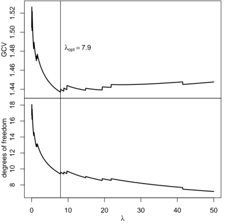
Now only the smoothing parameterλis left to be specified. It can be chosen for exam- ple by the (generalized) cross validation criterion (CV, GCV) or the Akaike information criterion (AIC) (e.g. summarized in Ruppert et al., 2003, Section 5.3). Several of these criteria are based on the elements of the diagonal of the hat matrix of the estimation.
Ruppert et al. (2003, Section 3.13) use the trace of the hat matrix of a penalized spline estimation as the equivalent to the degrees of freedom in linear models. For linear models, the degrees of freedom (df) are given by the number of parameters which in this case equals the trace of the hat matrix. Section 2.2 explains how to obtain the hat matrix for the spline estimators considered in this section.
For more details on spline estimation using the same notation see Kagerer (2013).
That work also covers the general case with one or more than one covariate which is considered in the next section.
2.2 A hat matrix for monotonicity constrained P-splines The hat matrixHof the minimization problem minf˜Pn
i=1(yi−f˜(xi))2withq×1 covariate vectorxi is defined to be the matrix for which ˆy=Hy. In case of a linear regression, i.e.
minα˜Pn
i=1(yi−xiα)˜ 2, withX=
xT1 · · · xTi · · · xTn T
, the hat matrix is given by
H=X(XTX)−1XT. (7)
For penalized estimations with a general symmetric penalty matrixD(for an example see Equation (11) below) wherePn
i=1(yi−xiα)˜ 2+λα˜TDα˜ is minimized with respect to
˜
α, the hat matrix can be determined as
Hλ =X(XTX+λD)−1XT (8) (e.g. Ruppert et al., 2003, Section 3.10).
For regression problems with general inequality constraints but without penalty, i.e.
minα˜Pn
i=1(yi−xiα)˜ 2 subject toCα˜ ≥0 (for an example see Equation (12) below), the hat matrix can be derived from the work of Paula (1999) and is given by
Hconstr =X I−(XTX)−1CTR(CR(XTX)−1CTR)−1CR
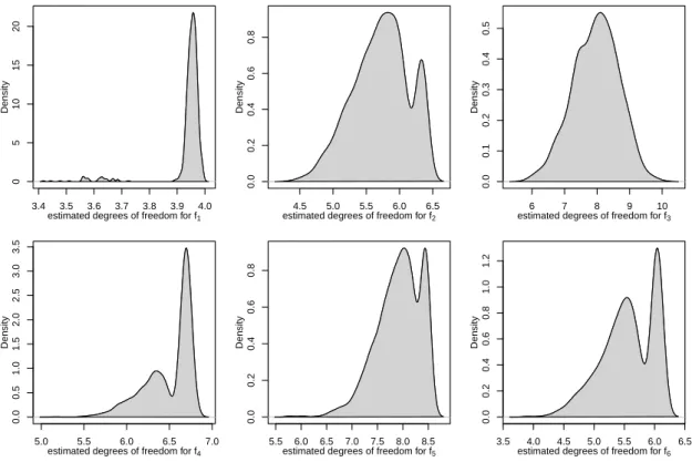
(XTX)−1XT, (9) where the q×r matrix CR contains ther rows of Csatisfying Cˆα =0 (cf. Paula, 1993, 1999). Since ˆα is a random variable, it is also random which rows of C satisfyCαˆ =0, henceCR and with itHconstr and its trace are random. This can also be observed in the simulation in Section 3 (e.g. Figure 5) and is also discussed in the empirical Section 4.
Penalized estimations with inequality constraints are obtained by minimizingPn i=1(yi− xiα)˜ 2 +λ˜αTDα˜ subject to C˜α ≥ 0 with respect to ˜α. Since the penalized estima- tion without constraints can be interpreted as ordinary least-squares problem with X∗ =
XT √
λ(D1/2)T T
and y∗ =
yT 0T T
(e.g. Eilers & Marx, 1996), these two hat ma- trices can be combined, resulting in the hat matrix for inequality constrained penalized estimations:
Hλ,constr =X I−(XTX+λD)−1CTR(CR(XTX+λD)−1CTR)−1CR
(XTX+λD)−1XT. (10) Note that for the hat matrices from the constrained estimations (9) and (10), CR is empty if the inequality constraint on Cαˆ is not necessary (i.e. none of the entries ofCαˆ is zero) and hence, the hat matrices reduce to the unconstrained case in (7) and (8).
Applying the properties of the trace operator, the trace of the hat matrix reduces to q(i.e. the number of estimated parameters) in case of the unconstrained unpenalized esti- mation (hat matrix (7)) and toq−rin case of the constrained but unpenalized estimation (hat matrix (9)). Hence for minα˜ Pn
i=1(yi−xiα)˜ 2 subject to Cα˜ ≥ 0, the degrees of freedom of the estimation equal the number of estimated parameters minus the number of rows of the constraint matrix C for which Cˆα = 0 holds. For the case of penalized estimations, the trace of the hat matrices (8) and (10) can not be simplified in an analog way and have to be determined after having estimated the model with the given data.
For penalized monotonicity constrained spline estimations ((5) with constraint (4)) with equidistant knots for a scalar covariatex, the (i, j)-th entry of then×(m+k) matrixX isBκ,kj−k(xi). The penalty matrixDis the matrix for whichPm
j=−(k−1)+2(∆2α˜j)2 = ˜αTDα˜ holds and hence is given by
D=
1−2 1
−2 5−4 1 1−4 6−4 ·
1−4 6 · · 1−4 · · 1
1 · · −4 1
· · 6−4 1
· −4 5−2 1−2 1
. (11)
Note that the penalty matrix can also be obtained for non-equidistant knot sequences (cf.
Kagerer, 2013).
The constraint matrix C required to satisfy the constraint (4) which results in a monotonically increasing fit is
C=
−1 1
−1 1
−1 1
... ...
(12)
and for a monotone decreasing fit it has to be multiplied by−1.
3 Monte Carlo simulation
3.1 Data generating processes
In this section only bivariate data generating processes (DGPs) are considered, i.e.
y=f(x) +u.
For all DGPs, the scalar covariate xand the errors u are assumed to be distributed as x∼U(0,1), u|x∼N(0, σ2).
To be able to use the same knot sequence for all replications, x is rescaled such that mini(xi) = 0 and maxi(xi) = 1 for each sample.
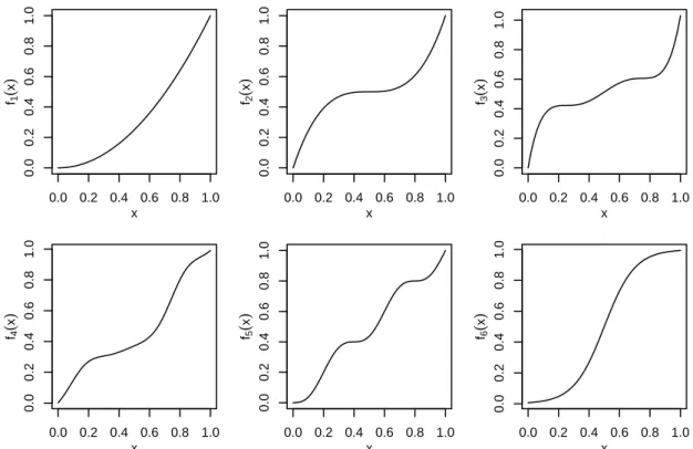
Six different regression functionsf are studied:
f1(x) =x2,
f2(x) = 4 (x−0.5)3+ 0.5,
f3(x) = 34.1x5−85.3x4+ 78.23x3−32x2+ 6x, f4(x) =
5
X
j=−3
αjBjκ,4(x)−0.2 forαT = 2 2 7 7 8 9 16 16 20 /14, f5(x) =x−sin(5π x)/16,
f6(x) = exp(10(x−0.5)) 1 + exp(10(x−0.5)).
The functions f1, f2 and f3 are polynomial functions of different degrees, f4 is a cubic spline, f5 is the sine function with higher periodicity and a trend and f6 is the CDF of the logistic distribution with parameters a = 0.5 and b = 0.1. All functions are chosen such that they are monotonically increasing on the interval [0,1]. Further, they are (ap- proximately) scaled on the interval [0,1], i.e. f(x) ∈ [0,1] for x ∈ [0,1], hence the same error variance σ2 is appropriate for all DGPs and is chosen to equal σ2 = 0.09. Figure 1 presents the respective functions and Figure 2 shows one simulated sample for each DGP.
For all estimations the open source software R (R Core Team, 2014, version 3.1.2, 32 bit) is used. The spline regressions are based on the base package splines and the constraint is implemented using the function pcls from the mgcv package from Wood (2014).
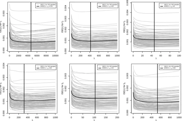
3.2 Simulation results
For each replicationr = 1, . . . , R, R = 1000, of the Monte Carlo simulation, a sample of size n = 500 is drawn for x and u and the corresponding y for the regression functions f1 tof6 are calculated. According to Equation (6), the knot sequence for the spline basis κ contains m = 35 equidistant inner knots and is subject to the constraint (4) for all functions f1 to f6. For each function the smoothing parameter λ has to be chosen. In the simulation the true functionf is known. Hence,λ can be selected for each of the six functions f from Section 3.1 by minimizing the mean integrated squared error (M ISE).