Regensburger
DISKUSSIONSBEITRÄGE zur Wirtschaftswissenschaft
University of Regensburg Working Papers in Business, Economics and Management Information Systems
Long- versus Medium-Run Identification in Fractionally Integrated VAR Models
Rolf Tschernig
, Enzo Weber
, Roland Weigand
December 2013
Nr. 476
JEL Classification: C32, C50
Key Words: Structural vector autoregression, long-run restriction, finite-horizon
identification, fractional integration, impulse response function.
*Rolf Tschernig holds the chair of Econometrics at the Department of Economics and Econometrics at the University of Regensburg, 93040 Regensburg, Germany.
Phone: +49-941-943-2737, E-mail: rolf.tschernig[at]wiwi.uni-regensburg.de
Enzo Weber holds the chair of Empirical Economics, especially Macroeconometrics and Labour Markets at the Department of Economics and Econometrics at the University of Regensburg, 93040 Regensburg, Germany, and is head of the research department Forecasts and Structural Analysis of the Institute for Employment Research (IAB), 90478 Nuremberg, Germany.
Phone: +49 -911-179-7643, E-mail: enzo.weber[at]iab.de
Long- versus medium-run identification in fractionally integrated VAR models
Rolf Tscherniga, Enzo Webera,b,c, and Roland Weigand∗b
aUniversity of Regensburg, Department of Economics, Universit¨atsstraße 31, D-93040 Regensburg, Germany
bInstitute for Employment Research (IAB), Regensburger Straße 104, D-90478 Nuremberg, Germany
cInstitute for East and Southeast European Studies, Landshuter Straße 4, D-93047 Regensburg, Germany
December 2013
Abstract. We state that long-run restrictions that identify structural shocks in VAR models with unit roots lose their original interpretation if the fractional integration order of the affected variable is below one. For such fractionally integrated models we consider a medium-run approach that employs restrictions on variance contributions over finite horizons. We show for alternative identification schemes that letting the horizon tend to infinity is equivalent to imposing the restriction of Blanchard and Quah (1989) introduced for the unit-root case.
JEL classification. C32, C50.
Keywords. Structural vector autoregression, long-run restriction, finite-horizon identifica- tion, fractional integration, impulse response function.
∗Corresponding author. Tel.: +49 911 179 3291.
E-Mail addresses:
Rolf.Tschernig@wiwi.uni-regensburg.de (R. Tschernig), Enzo.Weber@iab.de (E. Weber),
Roland.Weigand@iab.de (R. Weigand)
1 Introduction
Correct specification of integration orders is essential for valid inference in structural vector autoregressive (SVAR1) models, in particular, if identification of the structural shocks is related to their long-run effects. Therefore, the literature considered fractional time series models where the orders of integration may take on real (instead of integer) values and are estimated along with the other model parameters.
Recent results suggest that macroeconomic variables such as GDP or inflation may have integration orders smaller than one; see, e.g., Caporale and Gil-Alana (2013) or Gil-Alana (2011). This means that in multivariate fractional integration models, no shock could have an infinitely long-living effect on these variables, regardless of structural restrictions.
As a remedy we suggest the use of medium-run constraints for identification, which was considered in standard SVARs by Uhlig (2004) and Francis et al. (2013) as an alternative to long-run restrictions. We propose several approaches which constrain the variance contribution of selected shocks over a prespecified range of periods. For these finite-horizon criteria we show that by letting the number of periods tend to infinity they become formally identical to the computationally straightforward Blanchard and Quah (1989) condition. We thus provide an economic interpretation of the latter and justify its use in a fractional context.
2 Fractional SVARs and identification
2.1 The model
In order to avoid the restriction of integer integration orders for structural VAR analysis, fractionally integrated vector autoregressive (FIVAR) models have been used; see, e.g., Capo- rale and Gil-Alana (2011), Gil-Alana and Moreno (2009) or Lovcha (2009). Tschernig et al.
(2013) introduced additional flexibility for the short-run dynamics by a fractional lag operator.
The subsequent analysis will be based on the popular FIVAR model, noting that the results straightforwardly carry over to the more flexible model of Tschernig et al. (2013) as well. We assume that the bivariate time seriesxt= (x1t, x2t)0 is generated by
A(L)∆(L;d)xt=Bεt, t= 1,2, . . . , (1) where L is the lag or backshift operator (Lxt = xt−1) and ∆(L;d) := diag(∆d1,∆d2) holds the fractional difference operators ∆dj = (1−L)dj of real orders d1 and d2 (see, e.g., Baillie, 1996). Starting values are set to zero, i.e., xt =0 for t <1 although this assumption can be relaxed along the lines of Johansen (2008).
1Abbreviations used in the text: (S)VAR: (Structural) vector autoregression, FIVAR: Fractionally inte- grated vector autoregression, LRR: Long-run restriction, LRRS: Long-run restricted shock, LRUS: Long-run unrestricted shock
Analogously to standard non-cointegrated VAR models with unit roots, the fractionally differenced series (∆d1x1,t ∆d2x2,t)0 follows a stable VAR model with all roots of A(L) = I−A1L−. . .−ApLp outside the unit circle. In our structural setup, εt∼ IID(0;I) is the vector of economic shocks and the impact matrixB holds their contemporaneous effects.
2.2 Long-run and finite-horizon identification schemes
Identification restrictions are needed to uniquely recover the elements of the impact matrix B from the reduced-form error covariance matrix Ω = Var(ut) = BB0, where ut = Bεt
is the reduced-form disturbance term. To this end, Blanchard and Quah (1989) introduced the concept of long-run restrictions which exclude an infinitely long-lasting impact of selected shocks on a specific variable. In a setup with d1 = d2 = 1, denote Ξ(z) := P∞
j=0Ξjzj = A(z)−1B. The effect of a shock inεton xt+h in the distant future,h→ ∞, is given byΞ(1).
Identification of B can be obtained by constraining the permanent effect of, say, ε2,t on the first variablex1,t using the long-run restriction (LRR)
Ξ(1) =A(1)−1B = ξ11(1) 0 ξ21(1) ξ22(1)
!
. (2)
We keep this ordering of shocks and refer to ε1,t as the long-run unrestricted shock (LRUS), whileε2,t is called the long-run restricted shock (LRRS). Below we will show that in fractional models the LRR (2) loses its original interpretation but features the meaning of a medium-run restriction in the limiting case.
Letxt=Θ0εt+Θ1εt−1+Θ2εt−2+. . . denote the vector moving average representation of model (1), and denote byθij,h theijth element ofΘh, i.e. the impulse responses of theith variable to thejth structural shock at horizonh.2 Shocks tox1,t can have ever lasting effects on future realizations of this variable only if d1 ≥ 1. Formally, as established by Kokoszka and Taqqu (1995), the impulse responses generally evolve at a rate of order hd1−1 and thus converge to zero at a hyperbolic rate ifd1 <1. The impact ofany shock tox1,t vanishes with an increasing horizon so that no long-run effect in the terminology of Blanchard and Quah (1989) exists. The economic interpretation of LRR (2) is no longer obvious in this context.
To clarify this interpretation we apply an approach focussing on specified finite horizons and show how it can approximate the long-term behavior. To quantify the influence of the structural shocks for a given horizon, note that the forecast error ofxi,t+h,i∈ {1,2}, based on known coefficients and information up to periodtis given byPh−1
s=0
P2
j=1θij,sεj,t+h−s. Consider the forecast error variance
Vart(xi,t+h) =
h−1
X
s=0
θi1,s2 +θ2i2,s
=
h−1
X
s=0
θ2i1,s+
h−1
X
j=0
θ2i2,s, i= 1,2, (3)
2Chung (2001) discusses computation of impulse responses and their properties in the vector ARFIMA model while Do et al. (2013) introduce conceptually different generalized impulse responses in our FIVAR setup.
which can be decomposed into one variance component due to the LRUS,ε1,t, and one due to the LRRS,ε2,t. Thus, the share of the h-step forecast variance of variableidue toεj,t is given by
ωij,h =
Ph−1 s=0θ2ij,s
Vart(xi,t+h). (4)
In order to require a small impact of the LRRS on the behavior of the first variable h periods ahead, we consider three identification schemes which draw on restricting these variance shares or a variant thereof. We first choose an identification procedure that directly minimizes the forecast error variance share of the LRRS, i.e. FIN1
minB ω12,h s.t. BB0 =Ω. (5)
Since minimizing the contribution of the restricted shock amounts to maximizing the share of the unrestricted one, in our bivariate model this is identical to the constraint brought forward by Francis et al. (2013).
While economic theory hardly gives any guidance regarding an appropriate value of h, one may instead have an interval of horizons in mind which will be considered relevant. Then it would be reasonable to focus on a rangeh∈[l;u], over which the LRRS should have minimal impact. Using the average forecast error variance contribution (4) for identification yields FIN2
minB
1 u−l+ 1
u
X
h=l
ω12,h s.t. BB0 =Ω. (6)
If a shockε2,t has a large effect on x1,t over the first few periods, this is also reflected by the longer-term forecast error variance since short-horizon impulse responses enter FIN1 (5) and FIN2 (6) through the sum in (3). The interpretation of the LRRS as having a restricted effect over longer horizons may suffer from this property. In order to avoid this problem we modify FIN1 and obtain FIN3
minB
Ph i=lθ212,i
Vart(x1,t+h) s.t. BB0 =Ω, (7)
where now the variance share of exclusively the successive h−l shocks, ε2,t+1, . . . , ε2,t+h−l, contributing to ax1,t+h is minimized. The restriction proposed by Uhlig (2004) is obtained as a special case by settingl=hfor FIN3. The computation of all three finite horizon restrictions is described in Appendix A.
3 Relation between long-run and finite-horizon restrictions
3.1 The long and the medium run in fractional models
Without the typical interpretation, but still referred to as the LRR in the following, restriction (2) can be likewise imposed in the fractional model. Regardless ofB, the “long-run covariance
matrix”A(1)−1Ω[A(1)0]−1 is a function of reduced form parameters only. Using the Cholesky decomposition, this matrix can be uniquely written as Ξ(1)Ξ(1)0 due to the triangularity imposed on Ξ(1). The impact matrix B is then straightforwardly calculated as A(1)Ξ(1) which is exactly the same as in standard integrated VAR models.
The effect of the LRR in the fractional setting is not obvious: Tschernig et al. (2013) show that after technically imposing (2), one may write the first variable as
x1,t= [∆−d1ξ11(1) + ∆1−d1ξ11∗ (L)] [ε1,tI(t≥1)]
| {z }
θ11,0ε1,t+θ11,1ε1,t−1+...+θ11,t−1ε1,1
+ ∆1−d1ξ∗12(L) [ε2,tI(t≥1)]
| {z }
θ12,0ε2,t+θ12,1ε2,t−1+...+θ12,t−1ε2,1
, (8)
where theξ1j∗ (L), j = 1,2,are polynomials generating I(0) processes. This implies that θ11,h andθ12,h evolve at different rates for large horizons. Whileθ11,h∼hd1−1 is typical for impulse responses of I(d1) processes (see Chung, 2001), we observe a reduced rateθ12,h∼hd1−2 for the responses to the LRRS.
Hence, the LRR (2) and the finite-horizon restrictions yield qualitatively different results with respect to the rate of decay of the impulse responses: Only the LRR (2) affects the memory property of the LRRS-driven component of x1,t (the second term in (8)). In contrast, since ξ12(1)6= 0 for the finite-horizon conditions FIN1 (5), FIN2 (6) and FIN3 (7), these restrictions do not lead to differing rates ofθ11,h and θ12,h.
However, the rate at which the impulse responses θ12,h evolve is also the fundamental determinant of variance shares over longer horizons. Consequently, for the case d1 >0.5, we establish that identification by the restrictions FIN1 (5) and FIN3 (7) yields the same result as LRR (2) ifh→ ∞, while FIN2 (6) is equivalent for u→ ∞.
To see the asymptotic equivalence between the LRR and the finite horizon restrictions, let a scalarβ ∈[−1; 1] index the identification scheme (see (A.1) in the Appendix) so thatξ12(1;β) explicitly depends onβ. Letting the horizonhtend to infinity, it is shown in Appendix B that the objective function of FIN1 (5) fulfills
ω12,h−→ξ12(1;β)2
Γ(d1)2(2d1−1) lim
h→∞h1−2d1Vart(x1,t+h) −1
ash→ ∞. (9) The latter expression is minimized by taking β as to satisfy the LRR (2) because then ξ12(1;β) = 0 while the other terms are strictly positive. The same limit results for FIN2 and FIN3, since the difference between their objective functions and ω12,h is negligible for large horizonsu and h, respectively.
3.2 Practical implications
We assess the practical relevance of the previous result and the proximity of different identifying conditions for various values ofu and h for a stylized process with reduced form
"
1 0 0 1
!
− 0 −0.5 0 0.5
! L
# ∆0.7 0 0 ∆1.7
!
xt=ut, Ω = 1 0 0 1
!
. (10)
0 5 10 15 20 25 30
−0.20.00.20.40.6
Horizon
Impulse Response
FIN1
LRRh=1000h=100 h=20 h=5
0 5 10 15 20 25 30
−0.20.00.20.40.6
Horizon
Impulse Response
FIN2
LRRu=1000, l=0u=50, l=0 u=15, l=0 u=5, l=0
0 5 10 15 20 25 30
−0.20.00.20.40.6
Horizon
Impulse Response
FIN3
LRRh=1000, l=5h=50, l=5 h=15, l=5 h=5, l=5
0 5 10 15 20 25 30
−0.20.00.20.40.6
Horizon
Impulse Response
FIN2
LRRu=1000, l=5u=50, l=5 u=15, l=5 u=5, l=5
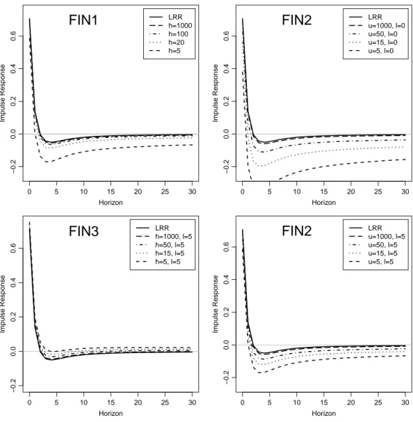
Figure 1: Impulse response function of the first variable to the second shock (LRRS) for the FIVAR process (10) and different identification restrictions imposed.
The integration orders are chosen according to the application to GDP and prices in Tschernig et al. (2013). The upper left panel of Figure 1 shows how the impulse response function of the first variable to the second shock (LRRS) depends onhfor the finite-horizon restriction FIN1 (5). With increasing horizon h, the FIN1-based impulse responses approach those resulting from the LRR. For h = 100 and larger the differences are negligible. Likewise, the impulse responses of shocks identified by FIN2 (6) and FIN3 (7), shown in the other three panels, also reveal that with growingu both restrictions yield results closer to the LRR (2), especially for the latter restriction and with larger values of l. While here the impulse responses become negative before they converge to zero, this behaviour could be avoided in the more flexible model of Tschernig et al. (2013), for which our results also hold.
In practice, the restriction LRR is thus justified and applicable not only with the long run defined by infinitely long horizons. If identification is meant to focus on the medium run but
with rather large horizons (in the present example, say, 50 upwards), the LRR can be taken as a good and technically straightforward approximation.
References
Baillie, R. T., 1996. Long memory processes and fractional integration in econometrics. Journal of Econometrics 73, 5–59.
Blanchard, O. and Quah, D., 1989. The dynamic effects of aggregate demand and supply disturbances. The American Economic Review 79, 655–673.
Caporale, G. and Gil-Alana, L. A., 2013. Long memory in US real output per capita. Empirical Economics 44, 591–611.
Caporale, G. M. and Gil-Alana, L. A., 2011. Fractional integration and impulse responses: a bivariate application to real output in the USA and four Scandinavian countries. Journal of Applied Statistics 38, 71–85.
Chung, C., 2001. Calculating and analyzing impulse responses for the vector ARFIMA model.
Economics Letters 71, 17–25.
Davidson, J., 1994. Stochastic limit theory. Oxford University Press.
Do, H. X., Brooks, R. D., and Treepongkaruna, S., 2013. Generalized impulse response analysis in a fractionally integrated vector autoregressive model. Economics Letters 118, 462–465.
Francis, N., Owyang, M. T., Roush, J. E., and DiCecio, R., 2013. A flexible finite-horizon alternative to long-run restrictions with an application to technology shocks. The Review of Economics and Statistics, forthcoming.
Gil-Alana, L. A., 2011. Inflation in South Africa. A long memory approach. Economics Letters 111, 207–209.
Gil-Alana, L. A. and Moreno, A., 2009. Technology shocks and hours worked: A fractional integration perspective. Macroeconomic Dynamics 13, 580 – 604.
Johansen, S., 2008. A representation theory for a class of vector autoregressive models for fractional processes. Econometric Theory 24, 651–676.
Kokoszka, P. S. and Taqqu, M. S., 1995. Fractional ARIMA with stable innovations. Stochastic Processes and their Applications 60, 19–47.
Lovcha, J., 2009. Hours worked - productivity puzzle: A seasonal fractional integration ap- proach. Unpublished manuscript.
L¨utkepohl, H., 1996. Handbook of matrices. Wiley & Sons.
Schotman, P. C., Tschernig, R., and Budek, J., 2008. Long memory and the term structure of risk. Journal of Financial Econometrics 2, 1–37.
Tschernig, R., Weber, E., and Weigand, R., 2013. Long-run identification in a fractionally integrated system. Journal of Business and Economic Statistics 31, 438-450.
Uhlig, H., 2004. Do technology shocks lead to a fall in total hours worked? Journal of the European Economic Association 2, 361–371.
A Computation of the impact matrix
For the computation of the impact matrixBsatisfying the finite-horizon restrictions FIN1 (5), FIN2 (6) and FIN3 (7), in the given setup any identification scheme (up to sign differences) can be indexed by a single numberβ ∈[−1; 1]. Here we use
B=P D= p11 0 p21 p22
! p1−β2 β
−β p 1−β2
!
, (A.1)
whereP is lower triangular and satisfies P P0 =Ω, whileD is orthonormal by construction.
Note that Vart(xi,t+h),i= 1,2, is independent ofβ and consider the variance component in (3) that is attributed to shock j. Denoting the reduced form MA coefficient matrices by Φh =ΘhB−1 and the unit basis vector with 1 in the ith row by ei, the impulse response of variableito shockj at horizon his given by
θij,h=e0iΦhP Dej =e0iΦhP dj, whered1 =
p1−β2
−β
!
, d2= β
p1−β2
! .
Hence, theh-step forecast variance shares are obtained by ωij,h =
Ph−1
s=0d0jP0Φ0seie0iΦsP dj
Vart(xi,t+h) =d0jVihdj. (A.2)
Since Vih is positive semidefinite and symmetric by construction, it can be represented as Vih=λ1v1v10+λ2v2v20 (L¨utkepohl, 1996, Section 9.13.3, Result (2)), whereλ1≥λ2 denote the nonnegative eigenvalues andv1,v2 the corresponding orthonormal eigenvectors, respectively.
It follows thatωij,h =λ1(d0jv1)2+λ2(d0jv2)2 with 0≤(d0jv1)2,(d0jv2)2 ≤ 1, where the latter property is due to orthonormality ofdj,v1 and v2.
Since both eigenvalues are nonnegative, the minimum ofω12,his obtained and thus restric- tion FIN1 (5) fulfilled ford1 =v1 and d2=v2. The impact matrix is computed as B=P D.
Analogously, FIN2 can be imposed by replacing Vih by the average ¯Vi,lu = u−l+11 Pu s=lVis, and FIN3 by using ˜Vi,lh=Ph−1
s=l P0Φ0seie0iΦsP instead.
B Proof of limit results
To obtain the result (9) note that from Chung (2001, Corollary 2) it follows that the squared impulse responses satisfy
θ12,j2 (β) = ξ12(1;β)2
Γ(d1)2 j2d1−2+o(j2d1−2).
Further, Schotman et al. (2008, eq. A20) state that Vart(x1,t+h) = Ch2d1−1+o(h2d1−1) with C >0, which does not depend on β.
Define
Xh(β) :=h1−2d1
h
X
j=1
θ12,j2 (β), Yh:=h1−2d1Vart(x1,t+h) and likewiseY∞:= limh→∞Yh >0. By Schotman et al. (2008, eq. A19) Pk
i=1iak−(a+1) k→∞−→
(a+ 1)−1 and therefore
h→∞lim Xh(β) = ξ12(1;β)2 Γ(d1)2
1
2d1−1. (B.1)
The result (9) follows fromω12,h=Xh(β)/Yh.
The same limit holds for FIN3 (7) with fixedl and h→ ∞because h1−2d1
h
X
j=1
θ212,j(β)−h1−2d1
h
X
j=l
θ212,j(β) =h1−2d1
l−1
X
j=1
θ212,j(β) =O(h1−2d1) =o(1).
The objective of FIN2 (6) is (u −l+ 1)−1Pu
h=lω12,h = u−1Pu
h=1ω12,h+o(1). Using Davidson (1994, Theorem 2.26), it satisfies
u→∞lim 1 u
u
X
h=1
ω12,h= lim
h→∞ω12,h as was claimed in the text.