Regensburger DISKUSSIONSBEITRÄGE zur Wirtschaftswissenschaft

(1)

Regensburger

DISKUSSIONSBEITRÄGE zur Wirtschaftswissenschaft

University of Regensburg Working Papers in Business, Economics and Management Information Systems

GDP-Employment Decoupling and the Productivity Puzzle in Germany

Sabine Klinger^*, Enzo Weber^**

April 27, 2015

Nr. 485

JEL Classification: E24, E32, J23, J24, C32

Keywords: decoupling, productivity puzzle, unobserved components, time-varying coefficient, Verdoorn´s law

* University of Regensburg, Department of Economics and Econometrics, 93040 Regensburg, Germany.

sabine.klinger@iab.de, and Institute for Employment Research (IAB).

** University of Regensburg, Department of Economics and Econometrics, 93040 Regensburg, Germany.

enzo.weber@wiwi.uni-regensburg.de, and Institute for Employment Research (IAB), IOS Regensburg.

(2)

GDP-Employment Decoupling and the Productivity Puzzle in Germany

Sabine Klinger (Institute for Employment Research (IAB), Nuremberg) Enzo Weber (Institute for Employment Research (IAB), Nuremberg, University of Regensburg and IOS Regensburg)

Abstract

This paper investigates the productivity puzzle in Germany. We focus on the time- varying relationship between German output and employment growth, in particular their decoupling in recent years. We estimate a correlated unobserved components model that allows for both persistent and cyclical time variation in the employment impact of GDP as well as an autonomous employment component capturing other factors than real output. As one result, we measure a permanent decline in GDP impact on employment as well as pronounced effects of the autonomous employment component in the recent years. The development of the estimated impact parameters depends on structural change, but also on labour availability and business expectations. Beyond GDP, a high labour supply, tightness as well as moderate wages and working time reductions boosted employment growth.

JEL classification: E24, E32, J23, J24, C32

Keywords: decoupling, productivity puzzle, unobserved components, time-varying coefficient, Verdoorn´s law

Acknowledgement

The authors would like to thank Jürgen Wiemers for valuable programming support.

Furthermore, we are grateful for comments to Christian Merkl as well as participants at the SNDE Symposium in Oslo, the ZEW Conference on Recent Developments in Mac- roeconomics in Mannheim, at the IAB-Bundesbank Conference Labour Markets and the Economic Crisis in Eltville, at the Applied Economics and Econometrics Seminar of the University of Mannheim, at the LMU Macro Research / CESifo Seminar, and at the Econometric Seminar of IAB and University of Regensburg.

(3)

1 Introduction

A few years after the acute phase of the Great Recession, models are more and more able to explain the driving mechanisms of the crisis and its spread-out (Christiano et al.

2014 as an example). Some of the effects turned out to be sustainable and revitalize the awareness of parameter instability (Ng/Wright 2013). Such permanent effects of the crisis are discussed in two main directions, unemployment hysteresis or Okun´s Law (Daly/Marks 2014, Canarella 2013, Pissarides 2013, Owyang/Sekhposyan 2012) and the productivity puzzle (Blundell et al. 2014, Barnett et al. 2014, Ball 2014). Our paper contributes to understanding the latter.

Output per worker unexpectedly rose during the Great Recession in the U.S. (Lucchet- ta/Paradiso 2014), whereas it fell and hardly recovered in Europe, e.g. in Great Britain or Germany. In general, the data do not fit the idea of a clear positive correlation between the growth rates of real output and per capita productivity (Verdoorn 1949). This result could be viewed from the supply side, analysing the production function and shocks to total factor productivity, capital intensity, and input utilization (Barnett et al.

2014, Pessoa/van Reenen 2013). Complementing these studies, we take a labour demand perspective and investigate the response of employment to output changes. We focus on Germany as a useful subject to study the productivity puzzle. Germany is the largest European economy with the reputation of being a highly productive location due to a comparatively large and high quality industrial sector. Moreover, after decades of sclerosis, its labour market experienced an internationally recognized upswing and performed extraordinarily well in the Great Recession.

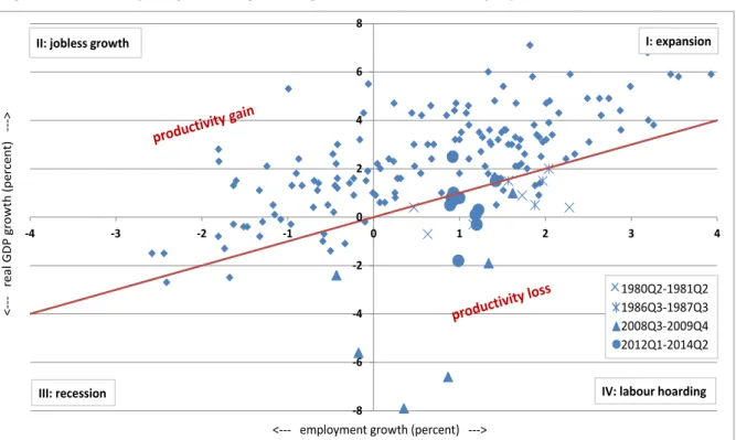
Figure 1 illustrates that expanding per capita labour productivity used to be the typical pattern in Germany; most observations lie above the line that indicates equal growth rates of GDP and employment. Productivity loss helped to absorb economic slumps as in 1980/81 and 1986/87, but such phases were exceptions – until the Great Recession.

The sharpest drop in GDP for decades caused hardly any reaction in employment. And not only did the Great Recession mark a sharp drop in productivity. Beyond the V- shape recovery, it also marks the beginning of a general slow-down in productivity growth. Further on, from 2011 to 2013, the Euro zone recession forced the German economy on fragile growth with utterly weak investment. Nevertheless, employers con- tinued to hire on balance. This behaviour was especially pronounced in the industrial sector.

At first glance, the rising trend in employment despite poor economic performance comes as a surprise. In order to shed light on the backgrounds, we address the following questions: a) How did the GDP-employment relation develop and is the development driven by structural or cyclical forces? b) How much do GDP growth and change

(4)

in GDP impact contribute to employment growth? Does the German labour market de- couple from GDP growth? c) Which are the determinants of time-variation in the GDP- employment relation? Or more pronouncedly, why do firms sometimes increase their staff despite poor economic performance and sometimes not?

Figure 1: Year-on-year percentage change of real GDP and employment, 1971 to 2014

Source: Destatis.

The first two questions are pursued by an analysis of the time-varying relation between employment and GDP growth. We study the German productivity puzzle from the perspective that labour demand is driven by output on the goods market. In that sense, the puzzle could arise from higher employment intensity of GDP (hypothesis 1) or from an overlay of the (less than) usual relationship by non-GDP factors (hypothesis 2). We estimate a time-varying coefficient whereby an increase of that parameter would confirm hypothesis 1, and a fall would confirm hypothesis 2.

Thereby, changes in the labour market reaction could be due to structural or cyclical reasons. “Structural” means a permanent consequence of shocks like the Great Re- cession or institutional or sectoral change. “Cyclical” means transitory impact changes due to the asymmetry of the business cycle as such (see e. g. Friedman´s plucking model in Friedman 1993, Kim/Nelson 1999a; Sinclair 2010) and due to asymmetric responses of the labour market to the cycle. Such asymmetry is found in Okun´s law, the relation between GDP and unemployment, as unemployment reacts more strongly to recessions than to expansions (e. g. Cevik et al. 2013, Holmes/Silverstone 2006, Silvapulle et al. 2004). These studies differentiate regimes but do not distinguish between cyclical and structural forces. Pereira (2013), Sinclair (2009), and Weber (1995)

-8 -6 -4 -2 0 2 4 6 8

-4 -3 -2 -1 0 1 2 3 4

<---real GDP growth (percent) --->

<--- employment growth (percent) --->

II: jobless growth I: expansion

III: recession IV: labour hoarding

1980Q2-1981Q2 1986Q3-1987Q3 2008Q3-2009Q4 2012Q1-2014Q2

(5)

consider trend and cycle of unemployment and GDP but do not consider asymmetric responses. Our paper bridges the gap in that we analyse parameter instability with respect to its permanent or transitory causes and separate the time-varying GDP effect from further driving forces of employment.

In order to distinguish between permanent and transitory effects, we estimate a time- varying parameter model and augment the previous literature (e.g. Kim/Nelson 1999b, Tucci 1995) by adding a cyclical component to the usual random walk. Thus, we con- struct a full unobserved components (UC) model (see e. g. Morley et al. 2003, Mor- ley/Piger 2012) for the TVP. This goes well beyond rolling window regressions as in Owyang/Sekhposyan (2012) and allows for high model flexibility, particularly with respect to whether the labour market reactions to GDP growth occur due to permanent or transitory reasons. Moreover, we apply a new identification strategy for the unobserved states as well as correlation of shocks in our UC-TVP model.

The third question regarding the determinants of the time variation points to developments beyond productivity which might solve the puzzle. Based on a search & matching framework we figure out potential explanatory variables. Among them, labour market tightness and the labour force established records recently as unemployment in Germany is the lowest and immigration is the highest since the early 1990s. Wage moderation and the spread of the service sector are further noticeable developments.

Some of them were influenced by the severe labour market reforms that came into force between 2003 and 2005. We check their contribution to explain the unforeseen rise in employment econometrically.

These are the main results: Labour productivity per capita has been falling since the Great Recession because weak GDP growth as the driver of employment growth was partially substituted by autonomous factors. Thereby, the reduction in GDP impact on employment growth is permanent, and the elasticity still remains at only half of the long-run average (which we estimate at 0.4, somewhat smaller than previous estimates in Leon-Ledesma 2000, Oelgemöller 2013). Furthermore, we find strong cyclical effects in the GDP-elasticity of employment. The development of the time-varying parameters depends on structural change and also on labour availability and business expectations. As determinants beyond GDP have gained importance in the labour market, recent employment growth would not have been possible if immigration and tightness had not been that high and if wage moderation and working time reductions had not taken place.

The details of our research are organized as follows: The next section provides a de- scription of our unobserved components model for the GDP-employment relation and sketch our identification and estimation strategy. The subsequent section presents the

(6)

results. Section 4 explains factors to rationalize time-variation and tests their relevance econometrically. Section 5 provides robustness checks. Finally, we summarize and conclude.

2 A correlated unobserved components model for time- varying GDP impact on employment

2.1 Before we start

As a starting point, consider a macroeconomic production function, for example of Cobb-Douglas type, Y_t A_tK_t^E_t^. Output Y depends on total factor productivity A, capital K, and employment E. Labour productivity is given as output per employed worker Y_t /E_t . Verdoorn (1949) states that this relation does not only depend on shocks to the production technology but also on output itself because higher output growth induces higher labour division and specialisation. This statement can be rein- terpreted as a dependence of employment on output growth (Kaldor 1966); we therefore name the parameter connecting the two “Verdoorn coefficient”.¹

A change in the relation of employment and GDP growth may imply a change in the effect of GDP on employment. This employment intensity of GDP growth could vary for structural as well as for cyclical reasons. However, the implication of varying GDP impact on employment is not mandatory. Certainly, the labour market is subject to a multi- tude of shocks that affect employment apart from current GDP fluctuations. These shocks may overlay and mask the real GDP impact. For instance, improvements of labour market institutions might reduce unemployment by faster matching independent- ly of the state of the business cycle. In this sense, e.g. Klinger/Rothe (2012) confirm the effectiveness of the Hartz reforms, but do not find a more than usual business cycle effect on matches. We therefore seek to disentangle the GDP impact on employment – which shows whether employment intensity of GDP growth has changed – and an autonomous component that may affect the empirical Y-E-relation separately from GDP growth or its impact.

The differentiation is essential: A high Verdoorn coefficient is beneficial during expansions but bears employment risks if the economy enters a recession. In contrast, autonomous labour market influences are principally not subject to such switches driven

1 In some studies (e.g. Blundell et al. 2014, Barnett et al. 2014), this relation is augmented to working hours. Our focus is on employment (as in Lucchetta/Paradiso 2014, Pessoa/van Reenen 2013). However, we consider working time in the empirical section as a relevant driving force.

(7)

by the business cycle. Moreover, it is also interesting for its own right to measure in how far labour markets are GDP-determined and in how far they follow influences from other sources. This leads us to a better understanding of the reasons and implications of the observations in the GDP growth–employment growth–space in Figure 1.

2.2 Model set-up

Kaldor´s representation of Verdoorn´s idea is a linear relationship between employment growth e_t and GDP growth y_t (equation 1). Empirical macro models regularly find the labour market lagging behind the development of GDP. Thus, we include q lags of GDP growth into the equation which implies q+1 Verdoorn coefficients _it^,^i=0,…,q,

t=1,…,T. Moreover, we include the autonomous component c_t^a that captures the time series dynamics of employment growth beyond GDP-dependent components. d92q1 represents a dummy variable for the German reunification. v_t is a white noise error term that avoids unsystematic effects being captured by the UCs.

(1) _t^a _t

q

i

i t it

t y c d q v

e 



   

  ₁ ₂ 92 1

0





Time variation is introduced by letting each Verdoorn coefficient consist of a stochastic trend _itand a cyclical component c_it (equation 2). Thus, the impact of GDP growth on employment growth may vary for permanent or transitory reasons. This is a crucial fea- ture since time variation can be governed by various factors such as structural or institutional change on the one hand and the regular asymmetry that has been found e.g. in Okun´s law on the other hand.

(2) _it_it c_it

The trends are modelled as random walks with drift _i and shocks _it (equation 3).

This allows for persistent stochastic change in the Verdoorn coefficients. Equation (4) specifies the transitory components as stationary autoregressions, which can capture various dynamic patterns. All roots of the lag polynomials in modulus lie outside the unit circle. We follow the standard UC approach (e.g. Morley et al. 2003, Sinclair 2009) and specify an AR(2), which is sufficient to enable cyclical fluctuations. Therein, _ij ⁽^{j =}

1, 2)are the autoregressive coefficients and _it are the cycle shocks.

(3)



_it 



_i



_i_,_t_1



_it

(4) c_it _i₁c_i_,_t_₁ _i₂c_i_,_t_₂ _it

(8)

A similar specification is used for the autonomous component (equation 5). While its persistence is not restricted a priori, this component empirically turns out to be stationary and is thus referred to as a cycle.

(5) _t^a

p

k a

k t a k a

t c

c 

 





 

1

In general, there is no reason to assume that the different UCs are independent of each other. Therefore, all trend shocks and all cycle shocks – including that of the autonomous cycle – are allowed to correlate. Such a correlated UC model in general provides a flexible framework avoiding assumptions not appropriate for the data at hand.

Equation (6) gives the covariance matrix for the residual vector

 

^

 _ot _qt _ot _qt _t^a _t

t v

u        .

(6)

 

















 

2 2 2

2

0 0

0

0 0 0

0

1 1 0

1 0 0 0

v t

t

a a q a

a q

a

u u E













 











As Figure 1 suggested, the Great Recession seems extraordinary with regard to the drop in GDP as well as the modest reaction of the German labour market. In order to specify the model flexibly enough to account for this extraordinary development, we allow the variances of all trend and cycle shocks of the TVP to break during that period, i.e. in the four quarters of negative GDP growth from 2008Q2 until 2009Q1. Particular- ly, this enables changes in the components of a size that is preferred by the data. Even more flexibility is achieved if we allow for similar behaviour through all recessions.

Thus, we include additional variance breaks in all economic downturns according to Schirwitz (2009). In the absence of an official business cycle dating in Germany, Schirwitz (2009) provides a comprehensive business cycle chronology based on several methods. This will be our preferred model; as a robustness check, we will limit our- selves to the one variance break during the Great Recession.

Although different trends and cycles of the TVP occur for each GDP lag, we suggest a summary in order to get an idea of the total impact of a GDP shock in a certain period.

Concretely, we summarize all trends _it, cycles c_it, and complete coefficients _it into one single trend 



^q 

i it i

t 0



,



, cycle 



^q 

i it i

t c

c 0 , , and Verdoorn coefficient



 

 ^q

i it i

t 0



,



. Thereby, the state value at time t reflects the total impact of a GDP growth shock at time t. It takes into account that the impact of this shock spreads out

(9)

until t+q. The summarized states will be the endogenous variables in the second-step regressions that investigate economic explanations for the development of the GDP impact on employment.

2.3 Technical issues 2.3.1 Identification

The challenge regarding identification is the need to recover multiple UCs from just one model equation. We begin with some intuition for why the specified model can be identified. In fact, all UCs can be uniquely determined: We distinguish the shocks to the Verdoorn coefficients by their persistence (permanent vs. transitory), the Verdoorn cycles from the autonomous cycle by the dependence on GDP of the former, and the autonomous cycle from the white noise shock by their autoregressive structure. Thus, all latent components have distinct characteristics.

Formally, we treat identification of our UC model by comparing the structural to the reduced form. Skipping the deterministic part for simplicity, the structural form of the model reads as follows:

(7) _t

a a t I

i

i t i

it I

i

i t it I

i

i t i

t v

y L y L

y L

e L 

 

 







 

 

) ( )

( 1

1 ₀ ₀

0







Therein, _i(L) (i=0,…,q) and _a(L)give the lag polynomials of the stationary TVP components as well as the autonomous cycle.

Next we derive the reduced form (equation 8). Therefore, equation (7) is multiplied by all lag polynomials including (1-L).

(8)

t a

q

i i a

t q

i i q

i

i t it a

q

i i i

i q

i

i t it a

q

i i q

i

i t i a q

i i t

a q

i i

v L L

L L

L

y L L

L

y L L

e L L

L





































































 







 





 



 



) 1 ( ) ( ) ( )

1 ( ) (

) 1 ( ) ( ) (

) ( ) (

) ( ) ( )

1 ( ) ( ) (

0 0

0 0,

*

0 0

0

*







The right hand-side of equation (8) consists of several MA terms. Some of their stochastic shocks are multiplied by time-varying GDP growth. This leads to heteroscedastic shocks on employment defined as _it_,_s _ity_s and _it_,_s _ity_s, which still have mean zero but non-constant conditional variances. I. e., a shock to the Verdoorn coeffi-

(10)

cient translates the stronger into employment, the larger current GDP changes. For identification, we can make use of an enriched set of information delivered by this heteroscedastic structure (compare Weber 2011). The reduced form is finally obtained by applying Granger´s Lemma (Granger/Morris 1976): The linear combination of the different MA terms results in a new composite MA term with the maximum lag length of the single MA components P(q1)2 p1^.

The autoregressive components as well as the drifts from the UC model can be gained directly from the reduced form, as can be seen from equation (8). The variances and covariances of the UC shocks must be recovered from the MA part, compare Morley et al. (2003). The heteroscedastic innovations on the RHS of equation (8) lead to time- varying autocovariances in the reduced form as well. Some information about the structure of this time variation is provided by the structural form: The (q1)2 p2^non- zero autocovariances consist of components that depend on either y_t__j^or y_t__j__iy_t__j (i=0,…,q and j=0,…,P+1) or do not depend on yt at all. Thus, we gain many pieces of information out of one autocovariance instead of just one. Consequently, we obtain more identifying equations than unknowns have to be estimated (29 variances and covariances of the UC shocks). Furthermore, it can be shown numerically that the coefficient matrix from the equation system has full rank 29. Thus, the structural form is identified.

2.3.2 Data, model specification, and estimation

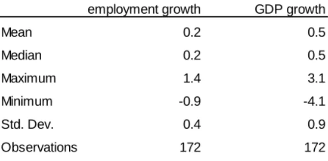
As far as the unobserved components model is concerned, we have very low data limi- tations. We use official seasonally adjusted qoq growth rates of real GDP and employment delivered by the German Federal Statistical Office from 1971Q1 to 2013Q4. Em- ployment covers all persons in dependent contracts regardless of their working time and professional status. The structural break of German reunification occurs in 1992Q1 and is captured by a special impulse dummy variable. Figure 2 shows the development of GDP and employment levels, Table 1 provides descriptives of the growth rates.

Table 1: Descriptive statistics, 1971Q1 to 2013Q4

Source: Destatis.

employment growth GDP growth

Mean 0.2 0.5

Median 0.2 0.5

Maximum 1.4 3.1

Minimum -0.9 -4.1

Std. Dev. 0.4 0.9

Observations 172 172

(11)

Figure 2: Level series of employment and GDP, 1971 to 2013

Source: Destatis. GDP is a price- and seasonally adjusted index with the base year changed at reunification (before: 1991=100, after: 2005=100).

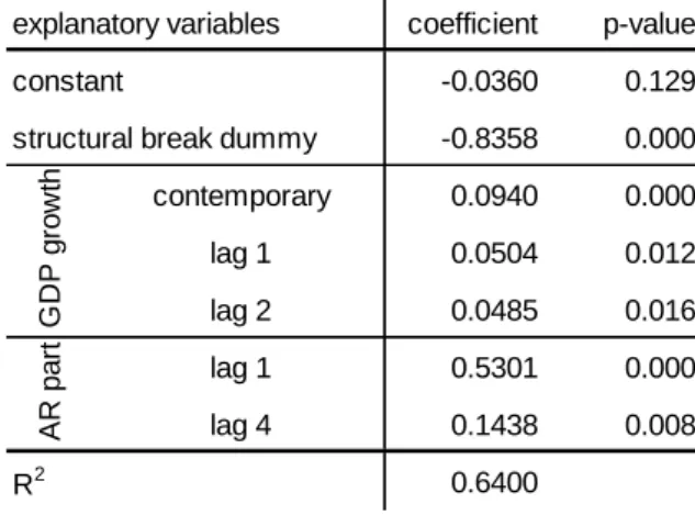
For the purpose of model specification, we first estimate the employment equation (1) as a constant parameter OLS regression, i. e. as a regression of employment growth on (lagged) GDP growth, own lags and deterministics (Table 2). Here, lag lengths could be chosen by the criteria of autocorrelation-free residuals and parameter signifi- cance. This provides us with a lag structure of GDP (q=2) and the autonomous component (p=4, with lags 2 and 3 being insignificant and dropped from the further analysis).

Moreover, we use the estimated constant Verdoorn coefficients as starting values for the TVP trends and the autoregressive coefficients as starting values for the autonomous cycle parameters. Starting values of the autoregressive coefficients in the TVP cycles as well as the trend and cycle shock variances are gained from an intensive grid search. As usual, the starting values of the covariances and cycles are set to zero.

Table 2: Constant parameter OLS regression of employment growth 20 40 60 80 100 120

15 000 20 000 25 000 30 000 35 000 40 000

1971 1976 1981 1986 1991 1996 2001 2006 2011

index points

1000 persons

Employment (left axis) GDP (right axis)

explanatory variables coefficient p-value

constant -0.0360 0.129

structural break dummy -0.8358 0.000

contemporary 0.0940 0.000

lag 1 0.0504 0.012

lag 2 0.0485 0.016

lag 1 0.5301 0.000

lag 4 0.1438 0.008

R² 0.6400

GDP growthAR part

(12)

We cast the model into state space form and apply maximum likelihood via numerical optimisation to estimate the parameters. Thereby, the likelihood function is constructed using the prediction error decomposition from the Kalman filter.

Residual diagnostics show that the model specification including the cycle lag lengths is a reasonable choice. We could neither reject the null hypothesis of no residual autocorrelation (Q-Test) nor the null hypotheses of no ARCH(1) effects (F-Test, Table 3).

Table 3: Model specification: autocorrelation and heteroscedasticity tests

3 Results: Time variation in the GDP-employment relation

3.1 Inspecting trend and cycle of GDP impact on employment

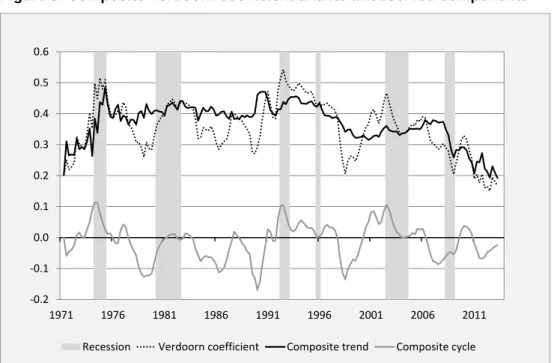
The estimated states of the TVP-UCs are given in Figure 3. The employment impact of GDP is positive all over the horizon. It experiences, however, trend increases and especially decreases as well as a pronounced cycle. The recessions according to Schir- witz (2009) are given in grey shade.

After a sharp increase around the time of the oil crisis, the trend in the Verdoorn coefficient kept a level of nearly 0.4 with slight fluctuations. The early 1990s saw a short increase². Afterwards, the trend decreased slowly until millennium. With the emergence of the new economy bubble it flattened again but slightly increased in the upswing before the Great Recession. The German labour market was announced for its mild response to the Great Recession (e. g. Burda/Hunt 2011), and Figure 3 reveals one of the reasons: trend impact of GDP dropped sharply such that the fall in GDP growth (by -4.1 % in the first quarter of 2009) was hardly passed through to employment. The total Verdoorn coefficient reached its first all-time low at this time. We emphasize that it is the trend that reacted to the crisis, not the cycle – even though the model would allow the latter to pick up a transitory recession effect. Nevertheless, a permanent reaction occurred, and the trend has not recovered ever since. Consequently, GDP impact has been at its lowest value for the whole period since 2011, when the Eurozone recession started to unfold. Section 4 will uncover economic reasons for this development.

2 This is not due to statistical effects from the German reunification – these effects occur in 1992 and are captured by a separate dummy variable in the measurement equation.

residual diagnostics p-value no AC until lag 1 0.288 no AC until lag 4 0.568 no ARCH until lag 1 0.708

(13)

Figure 3: Composite Verdoorn coefficient and its unobserved components

We conclude that the developments of GDP and employment growth decoupled to some extent. At least, the relationship is the loosest throughout the past 40 years.

Additional insight is gained from the new specification of a transitory TVP component (the result from a model without cycle is shown in the robustness section):

- The more flexible model demonstrates that the data prefer a permanent decline of the Verdoorn coefficient in 2009, indeed.

- There is a regular pattern related to GDP recessions.

- The cycle causes much higher variability of GDP impact on employment than would the trend alone.

- In specific phases, the cycle is as large as to change the classification of a recession and recovery as job-intensive or not.

We shortly elaborate on these issues. The cycle varies between -0.17 and +0.11. It is the main source of variation in the Verdoorn coefficient. The unconditional variance of shocks to c_t is more than twice as high as theunconditional variance of shocks to _t. The cycle exhibits six pronounced peaks, corresponding to an average cycle length of about seven years. The sum of the autoregressive coefficients of each single cycle

reveals that persistence (compare equation 4:

49 . 0

; 22 . 1

; 32 . 0

; 14 . 1

; 47 . 0

; 12 .

1 ₀₂ ₁₁ ₁₂ ₂₁ ₂₂

01          

 ). The composite

cycle peaks often coincide with the beginning of a recession. In four of the six recessions, we find the cycle dropping towards zero which implies that the transitory impact of a contraction on employment decreases. In other words, during recessions, the GDP impact on employment approaches its trend from above. This summary also holds for the beginning of the 1980s. However, as the cycle evolves from a negative value, it

-0.2 -0.1 0.0 0.1 0.2 0.3 0.4 0.5 0.6

1971 1976 1981 1986 1991 1996 2001 2006 2011

Recession Verdoorn coefficient Composite trend Composite cycle

(14)

rises during the first quarters of the recession and reaches its peak just then. The other outstanding case is the Great Recession. Although this was a phase of extraordinarily good labour market performance due to severe reforms as well as increased competi- tiveness of the German industry, the cycle does not show any extraordinary movement.

Over the whole horizon, the cycle and GDP growth (smoothed by a third-order moving average) correlate at -0.21; until the Great Recession the correlation was -0.38. The (moderate) negative empirical correlation reveals that German firms adjust employment modestly stronger to recessions than to expansions. This result is in line with the studies on asymmetry in Okun´s law.

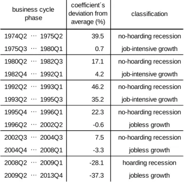
The sum of the TVP trend and cycle gives the total impact. Comparing this coefficient to its long-run average, we can classify the business cycle phases (pairs of recession and recovery) with regard to their specific employment reaction. For each phase, we calculate an average Verdoorn coefficient and its percent deviation from the long-run average. The sign of the deviation uncovers whether a recession came along with or without labour hoarding and whether the subsequent recovery was jobless or not. The absolute value of the deviation gives a hint on the strength of hoarding and job-intensity (Table 4).

Table 4: Business cycle classification by means of percent deviation of the Verdoorn coefficient from its long-run average

The recession and recovery shortly after reunification had the largest impact on employment. Since then, the damaging effect of recessions has declined but at the same time, recoveries started to become jobless. GDP growth did no longer translate into employment growth. The Great Recession and the recovery thereafter push this devel-

classification

1974Q2 … 1975Q2 39.5 no-hoarding recession 1975Q3 … 1980Q1 0.7 job-intensive growth 1980Q2 … 1982Q3 17.1 no-hoarding recession 1982Q4 … 1992Q1 4.2 job-intensive growth 1992Q2 … 1993Q1 46.2 no-hoarding recession 1993Q2 … 1995Q3 35.2 job-intensive growth 1995Q4 … 1996Q1 22.3 no-hoarding recession

1996Q2 … 2002Q2 -0.6 jobless growth

2002Q3 … 2004Q3 7.5 no-hoarding recession

2004Q4 … 2008Q1 -3.3 jobless growth

2008Q2 … 2009Q1 -28.1 hoarding recession 2009Q2 … 2013Q4 -37.3 jobless growth

business cycle phase

coefficient´s deviation from

average (%)

(15)

opment into extremes: The recession is classified as the only hoarding recession since the 1970s while the recovery thereafter seems to be outstandingly poor with regard to its transmission onto the labour market. The classification for the latest data is strongly driven by the drop in the coefficient´s trend. By contrast, the high trend as well as a positive coefficient cycle account for the strong employment reaction in the first half of the 1990s. Before reunification, the high trend was instead compensated by a comparatively large negative cycle. In other words, the employment effect of the expansion during the 1980s would have been substantially larger if its permanent component alone had been responsible for the impact. By contrast, the recession following the new economy bubble would have cost less jobs if the positive cycle had not turned it into a no-hoarding recession.

At first glance, the classification seems to contradict the impression in Figure 1: there, the economy did not only adjust to the Great Recession by productivity loss but to the recessions of the 1980s as well. Moreover, companies bear productivity loss in the current situation as well. The explanation is that the non-GDP component must be added to complete the picture. In fact, the autonomous employment cycle contributed to protecting employment in the recessions of the 1980s. By the same token, determinants beyond GDP must have gained importance in explaining the employment growth that occurred during the recent years.

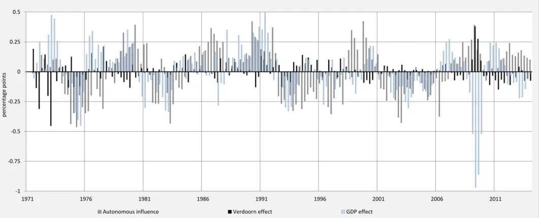
3.2 The role of GDP and autonomous drivers in employment growth The estimated Verdoorn coefficients allow us to decompose predicted employment growth (eˆ_t) into four components (equation 9): Three of them are related to GDP growth – first, the normal or sample average state; second, the Verdoorn effect that arises from mean-deviations of _it; and third, the GDP effect evaluated at an average Verdoorn coefficient. Finally, the autonomous effect presents the employment growth component beyond GDP.

(9) ˆ

   

( )

0 0

0

cons c

y y y

y

e _t^a

I

i

i t i t i I

i

i t i it I

i

i t i

t







 



  

  

 







  

The average effect is estimated at 0.17 – if the Verdoorn coefficient as well as GDP growth equal their sample means, employment will grow by 0.17 percent in each quarter, other influences being zero. Empirically, however, these other influences were not zero; they are depicted in Figure 4.

(16)

Figure 4: Decomposition of GDP and non-GDP impact on employment growth

-1 -0.75 -0.5 -0.25 0 0.25 0.5

1971 1976 1981 1986 1991 1996 2001 2006 2011

percentage points

Autonomous influence Verdoorn effect GDP effect

(17)

The decomposition shows a clear autonomous component with pronounced cycles (grey bars). It further reveals a high cyclicality of the GDP effect (light bars). Thus, much of employment growth volatility can be traced back to these fluctuations. Moreo- ver, the two effects exhibit a slight positive correlation and thus seem to go hand in hand on average – but not uniformly.

Above all, the picture is markedly different during the Great Recession and thereafter.

The extreme drop in the GDP effect was compensated commonly by the Verdoorn and the autonomous effects. Thus, the resilience of the German labour market during the Great Recession resulted from two factors. On the one hand, companies stopped translating GDP into employment decisions, i.e. they practiced typical labour hoarding.

On the other hand, institutional and structural change, particularly following the Hartz reforms, improved the functioning of the labour market and exerted positive effects on employment even through the crisis. For example, in the service sector, which was not severely hit by the crisis, employment steadily rose.

During the recovery from the crisis, the positive GDP effect is larger than the negative Verdoorn effect. However, if the Verdoorn coefficient had not fallen permanently, employment would have grown at higher rates. In 2011 to 2013, during the Euro zone recession, employment kept on rising mostly because of autonomous effects. Thereby, the autonomous component is not larger than before, but the positive correlation with the GDP effect is interrupted. Thus, during the latest years, factors beyond GDP did not support but substituted GDP as a determinant of employment growth, at least in large parts.

4 Explaining time variation by economic indicators

4.1 Variable selection

So far, we explain the productivity puzzle as a partial replacement of GDP impact on employment by factors beyond GDP that boost employment. In the following we dis- cuss potential sources of this time variation in the Verdoorn coefficient and the autonomous cycle. Variable selection is motivated by two fundamentals: first, a partial theoretical model of search & matching with endogenous separations (Pissarides 2000, Fujita/Ramey 2012) and second, an empirical sketch that detects remarkable developments of some of these key labour market variables.

The law of motion for employment is determined by matches M that raise employment, and separations S deteriorating employment (equation 10). Thus, any influence on these flow variables will affect employment change, the dependent variable in the first stage of the analysis.

(18)

(10) E_t M_tS_t

Matches are inflows into employment from any source. They are formed by the job finding rate multiplied by the number of job seekers. Thereby, the job finding rate is repre- sented by a matching function, often of Cobb-Douglas type and with constant returns to scale (Petrongolo/Pissarides 2001, equation 11). The latter assumption ensures that vacancies V and job seekers J can be summarized into labour market tightness

t t

t V /J

 . With matching efficiency m and elasticity of the job finding rate with respect to job seekers  , matches are given by

(11) M_t m_t



_t¹^^J_t

Separations consist of a group of exogenous dismissals or quits (as in the DSGE model by Christiano et al. 2014, for example) and a group of endogenously dismissed workers (e. g. Fujita/Ramey 2012, see our equation 12). Exogenous separations occur with separation rate s. Endogenous separations occur because i) a worker´s productivity is hit by an idiosyncratic shock with arrival rate



that leads to a new productivity below reservation productivity with probability G(R) or ii) reservation productivity changes such that a fraction of workers (Et-1(Rt) / Et-1) falls below even if they do not face a productivity shock (expressed by the complementary probability (1



)E_t_₁).

(12) S_t sE_t_₁



1s



G(R_t)E_t_₁(1)E_t_₁(R_t)



Reservation productivity is regularly derived from the endogenous job destruction condition (Pissarides 2000). A job is destroyed if its value is zero, i.e. if its return (productivity minus wages) is too low. We rewrite the job destruction condition without substi- tuting wages³:

(13) ⁰^ ^ ⁽ ⁾^ _



¹



^⁽ ^ ⁾^⁽ ⁽ ⁾^ ⁽ ⁾⁾



⁽ ⁾

R

n dG R w n w R n r p

R w

pR 



In sum, employment change would depend on the following factors, which we will investigate empirically: aggregate productivity (or output change) and job productivity, tightness, number of job seekers, matching efficiency, wages, and – in our model just for the deterministics – exogenous separation rate, productivity shock arrival rate and discount rate.

3 Typically, wages are replaced by the sharing rule of how a filled job´s surplus is distributed among the firm and the worker. This sharing rule would introduce more unknown parameters into our model which are hard to operationalize empirically, for example bargaining power.

Aiming at a macro-model, we prefer to stick to wages.

(19)

Aggregate output was dealt with on the first stage of the analysis. The theoretical con- siderations confirm that higher output boosts employment as it raises the return of a job and decreases reservation productivity. The other variables directly influence autonomous employment growth. Though, some of them could also influence the time-varying impact parameter because they may raise incentives to exploit GDP growth more or less intensively in terms of employment. This is subject to empirical investigation.

The aspect of labour hoarding – adjusting productivity, not employment to GDP – is captured in the integral of equation (13) without considering potential rehiring (Pissar- ides 2000, 44 f.): Firms keep unproductive jobs because further productivity shocks will arrive with probability



and might raise the job productivity to a new level n above reservation. In that case, the firm could start to exploit productivity immediately without searching for a new worker. The probability that a shock leads to job productivity below reservation (G(R)) would be conditioned on agents´ expectations if they possess relevant information about the future shock. If companies expect an economic recovery arriving soon they are likely to be more prone to labour hoarding. We check this kind of information by including an indicator of business expectations into our model.

Another rationale for labour hoarding (Bentolila/Bertola 1990; Horning 1994) is hardly mirrored in the search & matching model due to the free entry condition⁴: a tight labour market makes it time-consuming and costly to fill vacancies. The value of rehiring in comparison to the value of hoarding would increase incentives to reduce separations.

And it may also pay to enact precautionary hiring when tightness and hiring costs are high. We check these arguments empirically, including tightness as a measure of labour scarcity into the regression. The robustness section will provide further evidence on this kind of reasoning; it also mitigates worries about potential endogeneity.

While tightness is often referred to as vacancies over unemployed, we consider job seekers, or the labour force potential. This allows employment to grow from other sources than unemployment, especially from outside the labour force. The influential role of an increased labour force in explaining the UK productivity puzzle has been shown by Blundell et al. (2014). A high labour supply could reduce the incentive to hoard labour but increase the opportunity to recruit workers.

Matching efficiency summarizes factors that influence the functionality on the labour market, precisely how fast vacancies can be filled and unemployed find a job. The la-

4 With free entry and exit, the value of an additional vacancy is zero. But if there are frictions to market exit and if the market is still adjusting towards equilibrium, hiring costs matter for the value of the vacancy.

(20)

bour market reforms that came into force between 2003 and 2005 addressed search intensity, market flexibility and transparency. Previous research found that they contributed to a substantial (permanent) increase of matching efficiency (e.g.

Klinger/Weber 2014, Krebs/Scheffel 2013).

Wages determine the return of a job and therefore negatively influence job creation.

Moreover, they influence reservation productivity which has a direct positive impact on separations as well as an indirect effect via the probability that a new shock will de- grade job productivity below reservation. For instance, wage development reflects em- ployees´ shrinking bargaining power as trade union coverage has decreased and outside options worsened due to the Hartz Reforms (compare Dustmann et al. 2014, Krebs/Scheffel 2013 for Germany; Blundell et al. 2014, Gregg et al. 2014 for UK).

Any parameter in the model may differ by economic sector. As an illustrative example, the reservation productivity shall be smaller in services and higher in industries simply because of the technological infrastructure. Such heterogeneity makes the GDP impact on employment depend on the economic structure. This refers not only to persistent sectoral growth paths (Palley 1993) but also to transitory shifts stemming from the evo- lution of the production chain or factor substitution over the business cycle (Silvapulle et al. 2004).

We augment the variable list for the autonomous cycle by working time. This bridges the gap between productivity per capita, which is in our focus, and productivity per hour. Working time per employee is a substitute for employment to meet the demand for a certain volume of work.

4.2 The empirical model and data

To capture economic heterogeneity, we control for shares of sectoral gross value added. Perfect collinearity is avoided by skipping one sector (manufacturing). The service sector beyond trade/gastronomy/logistics and financial services/insurance contains business, public, information & communication as well as other services. Data is provided by the German Federal Statistical Office.

Labour market tightness is calculated as vacancies over unemployed, both published by the Federal Employment Agency. Starting after the labour market reforms until 2012, tightness had risen up to 17 vacancies per 100 unemployed while the average is 11 vacancies per 100 unemployed. The 2012 value was only exceeded in the late sev- enties and early nineties. Since then, tightness has been slightly shrinking.

Job seekers are captured by labour force potential, a business-cycle independent measure of potential labour supply, taking demography, migration, and participation

(21)

into account. The sharp increase in immigration – a balance of more than 400,000 people as in 2013 has not been observed since the early 1990s – as well as rising participation rates of women and older people outperformed the demographic decline in recent years. Labour force potential is calculated by the Institute for Employment Re- search (IAB) with yearly frequency; we interpolated the data.

Business expectations are an indicator based on regular survey responses of 7,000 enterprises on whether they anticipate their situation during the next six months to be more favourable, unchanged, or more unfavourable; it is calculated by the ifo Institute.

Wages have experienced a remarkable moderation since the end of the 1990s which was further sharpened after the labour market reforms. Meanwhile, they have started to rise again. We use total labour costs per hour including social contributions, published by the Federal Statistical Office.

Working time according to IAB data has been decreasing by trend, mainly due to an increase in the part-time ratio but also due to reductions in weekly working time negoti- ated in collective bargaining. Our measure also contains short-time work, a scheme widely used during the Great Recession to adjust labour without mass layoffs.

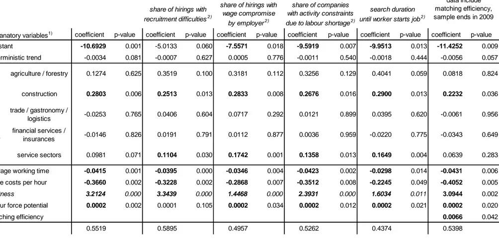
To summarize, the vector x_t contains the explanatory variables: shares of agriculture, construction, trade/gastronomy/logistics, finance and services in total gross value added, business expectations, tightness and labour force. Moreover, a second vector z_t equals x_t with business expectations excluded (as the autonomous cycle does not include GDP-related influences) and wages as well as working time included. The role of institutional change is checked in the robustness section because we have to rely on an own estimate of matching efficiency (Klinger/Weber 2014) which is only available at a shorter horizon.

Nonstationary series in the trend equation establish a cointegration relation. In the cycle equations, nonstationary series were differenced or captured by an explicit trend.

As described above, a large Verdoorn coefficient means high employment growth or high employment losses, depending on the sign of GDP growth. Thus, we allow the explanatory variables to have different impact on the trend and cycle of the Verdoorn coefficient (equations 14 and 15), depending on the sign of GDP growth. Beyond inter- cept and trend, we formulate the second-step regression models as

(14)



_t 



x_tD_tⁿ



*x_t(1D_tⁿ)



_t^

(15) c_t 



x_tD_tⁿ 



*x_t(1D_tⁿ)



_t^c (no differences for expectations and

tightness)

(22)

(16) c_t^a 



z_t 



_t^c^a (no differences for tightness and trend-stationary labour force potential)





 , and

denote the respective parameter vectors.



_tⁱ are white noise error terms.

The dummy variable D is set to 1 for negative GDP growth rates.







 

0 0

0 1

t n t

t if y

y D if

The parameters can be estimated by OLS using Newey-West standard errors for infer- ence. Data availability restricts us to run those regressions from 1992 onwards.

4.3 Results

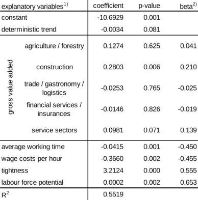
The results for the TVP second-step regressions are given in Table 5. The asymmetry due to positive / negative GDP growth proves especially reasonable with respect to the short-run TVP cycle. Most of the parameters change their sign, too, when GDP growth changes its sign. Regarding the long-run component of the coefficient, however, hardly any parameter changes its sign with respect to increasing / decreasing GDP. This finding is consistent with the idea of a permanent component: it does not routinely adjust to GDP changes. Once the effect is established, it continues to be effective in a similar manner over a long period. The details are interpreted in the following.

First, with respect to changes of the sectoral composition of the economy, we find that a persistent increase in the importance of the service sector (compared to manufacturing) by 1 percentage point in gross value added leads to a permanently lower GDP impact on employment by 0.04. This effect is temporarily strengthened (by 0.08) if an upswing comes through relatively higher service gross value added. By contrast, an importance gain in trade/gastronomy/logistics implies a permanently larger employment intensity of GDP growth by 0.04.⁵

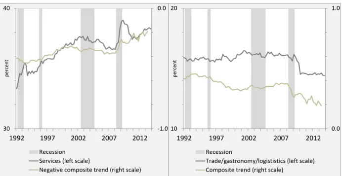
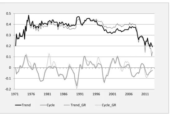
Figure 5 underlines the role of structural change. Employment volatility has always been stronger in industrial sectors. With the rise of the service economy, consequently, the GDP-employment relationship has become looser. This development was especially pronounced in the 1990s (compare Bachmann/Burda 2010 on the decisive role of sectoral change for the German labour market at that time) and during the Great Re- cession. Moreover, the share of the sector trade/gastronomy/logistics did not recover from the crisis – which seems to be one reason behind the drop in the TVP trend. Ob-

5 Furthermore, agriculture has a significant effect. However, the empirical relevance is low due to the small variations in this variable.

(23)

viously, while in Germany the Great Recession was quickly overcome, it left an imprint in the structure of the economy.

Table 5: OLS regressions for the time-varying Verdoorn coefficient

Figure 5: Trend of Verdoorn coefficient and the shares of gross value added of services as well as trade/gastronomy/logistics

Source: Federal Statistical Office, own calculation and estimation.

explanatory variables¹⁾ GDP growth coefficient p-value coefficient p-value

constant 1.0897 0.244 0.0705 0.528

deterministic trend -0.0008 0.334 -0.0006 0.018

> 0 -0.1177 0.000 -0.0228 0.836

< 0 0.0540 0.197 0.3374 0.147

> 0 -0.0005 0.949 -0.0539 0.202