DISKUSSIONSBEITRÄGE zur Wirtschaftswissenschaft
University of Regensburg Working Papers in Business, Economics and Management Information Systems
Decomposing Beveridge curve dynamics by correlated unobserved components
Sabine Klinger*, Enzo Weber**
May 9, 2014 Nr. 480
JEL Classification: C32, E24, E32, J2, J69
Keywords: Beveridge curve, worker flows, tightness, unobserved components, Hartz reforms
* University of Regensburg, Department of Economics and Econometrics, 93040 Regensburg, Germany.
sabine.klinger@iab.de, and Institute for Employment Research (IAB).
** University of Regensburg, Department of Economics and Econometrics, 93040 Regensburg, Germany.
enzo.weber@wiwi.uni-regensburg.de, and Institute for Employment Research (IAB), IOS Regensburg.
by correlated unobserved components
Sabine Klingera,b, Enzo Webera,b
a) Institute for Employment Research, Regensburger Straße 104, 90478 Nuremberg, Germany (sabine.klinger@iab.de, enzo.weber@iab.de)
b) University of Regensburg, Institute for Empirical Economic Research, Universitätsstraße 31, 93053 Regensburg, Germany
Abstract
Between 1979 and 2009, the German labour market moved along a Beveridge curve with changing slope that used to shift outwards but shifted inwards after severe labour market reforms had come into force. We analyse these dynamics and focus on the macroeconomic outcome of the reforms. For that purpose, we construct a new empirical model that links equilibrium unemployment theory to a flexible unobserved components model: we
disentangle permanent and transitory components of matching efficiency and separation rate as well as unemployment and vacancies. Cointegration and identification are addressed. We find that matching efficiency and separation rate each account for about half of the inward shift. Thereby, the increase in trend matching efficiency is extraordinary and testifies to a permanent improvement on the labour market. Its visibility, however, was retarded by an overlay with a structural increase in tightness.
Keywords: Beveridge curve, worker flows, tightness, unobserved components, Hartz reforms JEL: C32, E24, E32, J2, J69
Corresponding author:
Dr. Sabine Klinger, Institute for Employment Research, Federal Employment Agency, Regensburger Str. 104/We 115b, 90478 Nuremberg, Germany, sabine.klinger@iab.de, phone 0049-911-1793255.
1 Introduction
Economists used to describe the German labour market by rigidity, sclerosis and hysteresis as labour market flows were much lower than in the United States and unemployment became persistent over time (Blanchard/Summers 1986, Nickell 1997). Consequently, the German Beveridge curve (BC) – the downward sloping relationship between vacancies and
unemployment – shifted outwards. After a set of severe labour market reforms had come into force in 2003 to 2005, things started to change. The BC shifted inwards for the first time in decades. Following the standard interpretation (see the BC as a tool of macroeconomic policy analysis in Abraham/Katz (1986) and Blanchard/Diamond (1989)), this inward shift indicates a structural improvement of the functioning of the labour market. By contrast, the Great Recession 2008/09 just caused a limited and seemingly ordinary movement along the curve.1 We analyse the dynamics of the BC (see also Barnichon/Figura 2011, 2012, Bouvet 2012, Daly et al. 2012) with special focus on the macroeconomic outcome of the labour market reforms. For that purpose, we construct a new empirical labour market model. It directly connects to theory and allows us to address important issues with respect to the German BC:
We will find out about the empirical relevance of the theoretical driving forces of BC shifts and movements along the curve, foremost matching efficiency, the separation rate and labour market tightness. Thereby, it is of special interest – also from a policy perspective – whether these driving forces changed for structural or cyclical reasons, i.e. whether the functioning of the labour market improved permanently or just temporarily. This question gains special importance as common wisdom – shifts of the BC reflect structural change whereas movements along the curve are cyclical – will be challenged by our results (compare also Börsch-Supan 1991, Kosfeld et al. 2008, Fujita/Ramey 2009 or Davis et al. 2010).
1 This is in striking contrast to the development of the U.S. labour market, for instance, where unemployment rose sharply, long-term unemployment doubled, and the BC shifted outwards (Benati/Lubik 2014, Lubik 2013, Daly et al. 2012, Sala et al. 2013).
Furthermore, we seek to uncover how driving forces and labour market variables interact and how different permanent and cyclical processes interfere in the development of the BC (Blanchard 1997).
In our setup, we combine the theoretical framework of the BC and equilibrium unemployment with the flexibility of a correlated unobserved components model (for the latter, compare Morley et al. 2003). Particularly, we integrate a matching function into an unobserved
components framework (compare Dixon et al. 2014, Sedláček 2014). The model disentangles each of the key variables (unemployment, vacancies) and each of the shifting parameters (matching efficiency, separation rate, employment) into their unobserved permanent and transitory components; see King (2005) for another application to labour market flows. The permanent component – a completely persistent stochastic trend – reflects structural change whereas the transitory component is a mean-reverting trend-deviation. This methodology is especially advantageous for several reasons: The theoretical BC as a steady state relation implies cointegration between the series involved. In our framework, we are able to
implement this common trend exactly for the long-run components. Thereby, the model can combine two features: on the theoretical side, we integrate the long-run equilibrium while on the empirical side we avoid the usual problem – see e. g. Elsby/Hobijn/Sahin (2013) – that observed unemployment might be a bad approximation for equilibrium unemployment.
Moreover, the model can represent complex interactions in the labour market by allowing for correlation between all trend and cycle shocks. Additionally, we can investigate whether the impact of unemployment and vacancies in the matching function differs with respect to trend or cycle.
As the main results we show that matching efficiency and separation rate each contributed for about 50 percent to the inward shift. While the separation rate has been more important in explaining shifts of the BC over the whole horizon, matching efficiency experienced an outstanding upturn in the aftermath of the labour market reforms. This adds to studies that
confirm the positive influence of the reforms on matching efficiency (Fahr/Sunde 2009, Klinger/Rothe 2012, Hertweck/Sigrist 2012). The functioning of the labour market improved for structural reasons, indeed: It is the permanent component of matching efficiency – besides the permanent component of the separation rate – that firms up the inward shift, but with delay. The reason for this delay is a contemporary increase in trend tightness: the number of the unemployed shrank due to higher matching efficiency and lower separation rate, and the number of vacancies increased as firms profited from higher market transparency, wage moderation, and worse outside options of the employees. This argument is confirmed by a positive correlation between shocks to the trend components of matching efficiency and tightness. Thus, the overlay of several labour market reactions to the reforms leads to two parallel movements: the BC shifted inwards and the position on the curve moved upwards.
Within the matching function, trend and cyclical unemployment are of similar importance for match formation whereas it is only the cyclical component of vacancies that plays a
significant role.
The remainder of the paper is organized as follows: In the next section, we shortly introduce the development of the empirical BC in Germany and describe why the so called Hartz reforms should have been able to improve the functioning of the labour market, i. e. induce the BC´s inward shift. Next, we summarize the theoretical and empirical literature on why BC components, especially matching efficiency and separation rate, should vary permanently or/and transitorily. Section 4 describes our model. Afterwards, we briefly address
identification and estimation strategies and the data. In section 7, we interpret the results on the unobserved components and present the extended matching function. Finally, we summarize the paper and draw conclusions.
2 The Beveridge curve and the Hartz Reforms
Sclerosis and hysteresis used to be remarkable characteristics of the German labour market.
Over decades, unemployment rose stepwise and became persistent. The BC displays this worsening labour market situation by several shifts outwards and movements downwards along the curve (Figure 1).
Figure 1: The German Beveridge curve, 1979 to 2009
Source: Federal Employment Agency, data manipulation see text. Bullets refer to January of indicated year.
In the early 1980s, the German labour market experienced a quick and sharp decline in vacancies and increase in unemployment which makes the impression of a movement along a BC to its lower right edge. Afterwards, the BC steepened considerably. Thus, already before the German reunification, it became harder to exploit an increasing number of vacancies to reduce unemployment. Reunification itself caused a substantial right shift as a high number of workers became unemployed in the course of the transition of Eastern Germany towards a market economy. (We already adjusted for purely statistical effects.) The outward shift cannot only be attributed to the direct effects of the transition as it kept on until 2005. Moreover, this shift can be similarly observed in all federal states of Germany (Bouvet 2012) – it is not a
1100 1150 1200 1250 1300 1350
1350 1400 1450 1500 1550
ln(vacancies)*100
ln(unemployment)*100 1980
1983 2009
2004 2001
1995 1992
1986 1989
1998 2007
purely Eastern German phenomenon but must be rationalized by structural, e. g. institutional reasons that prompt unemployment to persist.
Mass unemployment with a high share of long-term unemployment caused the government to launch the most serious labour market and social reforms in German post-war history. The so called Hartz reforms consisted of four laws and came into force in three waves between 2003 and 2005. It concerned many components which can be summarized into three main targets (Jacobi/Kluve 2007, Klinger/Rothe 2012):
- First, higher efficiency in placement services targeted on the interaction of supply and demand. The former public employment service was re-organized with the aim of providing market-conform placement services, increase transparency about vacancy and worker profiles and establish a market-segmentation with specific support.
- Second, increasing activation and personal responsibility targeted on labour supply.
The reforms increased the incentives to search for a job more intensively and to be ready to take concessions. The period of entitlement to unemployment benefits was shortened and means-tested unemployment assistance for people without claims against unemployment insurance was lowered. Further reform components in that category are a stricter definition of reasonable work, implementing sanctions and target agreements regarding search effort as well as a new kind of start-up subsidy.
- Third, labour demand was to be boosted by allowing for higher flexibility, for example with respect to temporary agency work, employment protection legislation and
marginal employment.
These features are considered to improve the BC position (Bouvet 2012). Moreover, labour demand was stimulated by a moderate wage development as the outside options of employees worsened through the reforms (Krebs/Scheffel 2013). Starting in late 2006, the BC shifted inwards for the first time in decades.
The inward shift came to an end in late 2008 when the Great Recession hit the German labour market. Its response to a drop of GDP by more than 5 percent was notedly moderate. Labour demand did not drop as much as might have been expected based on the experience from previous recessions. This calls for another or a new structural effect that could have overlaid the crisis period and that does not show up in a shift of the BC but in a just modest movement along the curve.
3 Trend and cycle of Beveridge curve components
The BC is theoretically derived in the labour market model popularized by
Mortensen/Pissarides (1994) and surveyed in Pissarides (2000). The law of motion of
unemployment and the matching function lead to the BC as a downward sloping steady-state relation between vacancies and unemployment (see Figure 2).
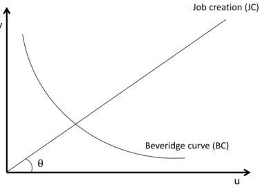
Figure 2: The stylized Beveridge curve
Source: Pissarides (2000), 20.
The exact position on the BC is marked by the intersection with the job creation curve (JCC).
Its rotations are reflected by changes in labour market tightness θ (vacancies over unemployment, the angle in Figure 2). An upper-left position on the curve indicates a relatively high number of vacancies and a relatively low number of unemployed. Then, the
v
u Job creation (JC)
Beveridge curve (BC)
labour market is tight, and firms may find it difficult to fill vacancies. The opposite holds in lower-right positions on the BC.
Two of the variables forming the intercept are matching efficiency, i. e. the efficiency component of the job finding rate that includes search intensity as well as public and private job placement, and the separation rate (see the model in section 4). In our analysis, the hazard rates give the probabilities of either finding a job out of unemployment or losing or quitting one´s job and transitioning into unemployment. Thus, one can regard them as chances and risks in the labour market. Changes to them cause shifts of the Beveridge curve.
Following common wisdom (e. g. Blanchard/Diamond 1989 and the subsequent literature), shifts of the BC are ascribed to changes in labour market trends caused by changes in institutions, technology, the sectoral composition of the economy, or demography. These shifts of the BC imply a change in the permanent component of unemployment, often named
“structural”. On the other hand, cyclical variation as a consequence of fluctuating productivity rotates the job creation curve (JCC) such that movements along the BC were considered to be cyclical.
This traditional view is not beyond doubt, however. Several authors put forward arguments that issue the cyclicality of matching efficiency, for example (Börsch-Supan 1991, Kosfeld et al. 2008, Fujita/Ramey 2009, Davis et al. 2010). In line with those authors we argue that basically all determinants of Beveridge curve dynamics may vary for permanent and transitory reasons. In other words: Shifts could occur not only for structural but also for cyclical reasons. Movements along the curve could occur not only for cyclical but also for structural reasons. We give important examples in the following.
To begin with, trends in matching efficiency, separation rate, and tightness occur because of structural – institutional, demographic, technological, sectoral – change (compare
Blanchard/Diamond 1989, Börsch-Supan 1991, Blanchard/Wolfers 2000, Davis/Haltiwanger
2001, King/Morley 2007, Boeri 2011, Barnichon/Figura 2012, Bouvet 2012). The most remarkable change in German labour market institutions – the Hartz reforms that started a decade ago – has been described in the previous section. Their effect on matching efficiency was positively evaluated (Fahr/Sunde 2009, Klinger/Rothe 2012, Hertweck/Sigrist 2012).
Permanent effects on the separation rate have not yet been investigated directly. As a hint, Rebien/Kettner (2011) state that after the reforms employees have become more willing to make concessions regarding their working conditions. At the same time, the share of labour market transitions that happen and are reversed within just one month may have increased (Nordmeier 2012) which reconciles higher institutional flexibility with shrinking separation rate in the data.
Matching efficiency and separation rate are determinants of labour market tightness, IOW of the slope of the job creation curve (for a derivation see Cahuc/Zylberberg 2004). Thus, their permanent components are carried over to that part of the Beveridge curve dynamics that used to be described as cyclical. Furthermore, permanent wage moderation (and dispersion) may lead to higher profitability of filled vacancies. The consequence would be a trend increase in tightness which shows up as a permanent movement up the BC. Such developments of wages could stem from a lower degree of unionization or worsened outside options after the reforms (see Dustmann et al. 2014 and Scheffel/Krebs 2013 for relevance in Germany).
On the other hand, cycles in the separation rate and tightness are brought in as spillovers of cyclical fluctuations of productivity. Cycles in matching efficiency occur because firms and workers adjust their search behaviour to those productivity fluctuations: recruiting or search intensity is adjusted as competition for (good) workers or firms (Davis et al. 2010, Davis 2011) and the average job finding probability of the unemployed vary over the business cycle (heterogeneity hypothesis, see Darby et al. 1985, Barnichon/Figura 2013, Sedláček 2014).
Furthermore, cyclical variation in the search and matching model has induced a large amount of studies with regard to the unemployment volatility puzzle (e. g. Shimer 2005, Fujita/Ramey
2005, Hagedorn/Manovskii 2008, Pissarides 2009). As part of this – basically microeconomic – debate, the countercyclicality of the separation rate was shown to be substantial and
influential for unemployment dynamics (e. g. Fujita/Ramey 2009, Elsby et al. 2009, and for Germany Nordmeier 2012, Hertweck/Sigrist 2012).
As a consequence of the aforementioned arguments, we employ an empirical strategy to simultaneously identify potential trends and cycles in all determinants of BC dynamics.
4 The model
In this section we develop our labour market model that will serve to analyse the BC dynamics, especially concerning the Hartz reforms. We follow the search and matching literature regarding theoretical key features (Mortensen/Pissarides 1994, Pissarides 2000, Petrongolo/Pissarides 2001 on the matching function) and integrate them into a flexible unobserved components specification.
Initially, we focus on the long-run equilibrium relations on the labour market. In empirical work, such theoretical equilibria are often operationalised by (linear) relations between observed time series although these do not only contain long-run information and,
consequently, do not appropriately reflect the market being in equilibrium.
Elsby/Hobijn/Sahin (2013) and Nordmeier (2012) argue that especially on the German labour market actual unemployment may be an insufficient approximation of equilibrium
unemployment. We will circumvent these problems by explicitly anchoring the steady state to the (unobserved) permanent components because it is their structural interrelations that are uncovered by the economic equilibrium. Thus, they form the cointegrating relation.
Steady state unemployment is achieved in the long-run flow equilibrium, i. e. if equilibrium matches and equilibrium separations equate. Thereby, following Pissarides (2000) and Shimer (2005), matches M and separations S are defined as transitions between employment and unemployment.
(1) M S
All variables are given in logarithms. Econometrically, expression (1) implies cointegration between separations and matches if the observed series are I(1).
Matches are formed by unemployed persons from U who leave unemployment with a certain probability, the job finding rate f, which at least partly mirrors labour market institutions.
Similarly, separations can be referred to as employees from E losing or quitting their job with a certain probability, the separation rate s. Changes in the hazard rates reflect the economic behaviour of agents, e. g. firms´ decisions on how many people to employ or dismiss. By contrast, the flow variables are subject to mere level effects due to changes in the stocks of unemployment and employment. We therefore rewrite the flow equilibrium (1) in terms of the long-run components of the log-linearized hazard rates and respective stock variables. The long-run component of unemployment U can be seen as some measure of structural unemployment, in theory often connected to the concept of the NAIRU.
(2) f U sE
The model does not assume a constant labour force. Although our analysis focusses on transitions between unemployment and employment, the equilibrium relation (2) does not involve the assumption that employment rate and unemployment rate form a direct
relationship and add up to 1, not even with regard to the given long-run values. These stocks may well vary because of transitions into or from further labour market states as well as out of the labour force. Moreover, as soon as such further transitions induce composition effects that affect matching efficiency or separation rate, they will enter our analysis implicitly. Finally, as equation (2) just reinterprets the flow equilibrium (1) and as neither the stocks nor the hazard rates are stationary, all four filtered trend series share a cointegration relation.
Equation (2) is the first step for the derivation of the BC. The second step is provided by the matching function that explains job finding probability depending on unemployed U and vacancies V. We specify a log-linear Cobb-Douglas-type matching function.
(3) f m
1
U Vm denotes matching efficiency while α and β are elasticities of matches with respect to
unemployment and vacancies, respectively.
Integrating (3) into (2) and rearranging gives the BC as steady state combinations of vacancies and unemployment.
(4) V
s E m
U
1
Shifts of the BC are caused by changes of the intercept. Therefore, inward shifts occur if c. p.
the separation rate or employment shrink and if matching efficiency or the elasticity of matches with respect to vacancies rise. The slope of the BC is determined by the two match elasticities.
So far, the derivation of the BC relied on the long-run components of the constituting variables. In reality, however, those long-run components are not observable. Instead, empirical BCs consist of time series that include long-run (persistent) and short-run (transitory) components. To disentangle these components we develop a correlated
unobserved components model. Thereby, each variable is decomposed into a stochastic trend
that captures permanent effects and a stationary autoregression that captures transitory effects (the cycle c, see equations 5 to 8). The focus of our paper is on matching efficiency and separation rate as they mirror behaviour and institutions that (might) have changed after the labour market reforms. We aim at specifying the time-varying properties of these
parameters.
As matching efficiency itself is not observable, we include the unobserved components specification into an empirical matching function (with the job finding rate f, matching efficiency m, unemployment U, vacancies V, the respective elasticities α and β, and a white noise error term w):
(5) m
t m t t
t t t
t t
c m
w V U
m f
1) 1 1
(
The stock variables are lagged in order to ensure that we appropriately model the time pattern of the unemployed getting registered first and potentially induce an outflow afterwards. In line with the specification of matching efficiency, we also allow for a stochastic trend and a cycle in the separation rate; see equation (6). The same applies to employment and vacancies.
This flexible specification has the advantage that it lets the data speak when determining the nature of labour market processes.
(6)
V t V t t
E t E t t
s t s t t
c V
c E
c s
As an important feature of our model, the steady state Beveridge relation (4) summarizes five nonstationary variables into one equilibrium relation. Therefore, it implies cointegration: At most four stochastic trends can be independent. Consequently, we use the Beveridge relation to specify the permanent component of our remaining variable, unemployment2, as a
composite trend of employment, separation rate, matching efficiency, and vacancies (and besides control for a deterministic trend and an intercept); see equation (7). The specification of a common trend would not have been possible with a smoothing filter like HP. Our
approach achieves two important goals: First, we can appropriately integrate the restriction stemming from the BC into our model. Second, since this restriction applies only to the long-
2 Econometrically, choosing one of the other variables would just imply a linear transformation not altering the model.
run components, we do not have to rely on the poor approximation of equilibrium unemployment by the actual values – the cycle components are still unconstrained.
(7)
UtV t E t s t m t
t c
U
1
The inclusion of vacancies as an endogenous variable (see equation 6) closes the model. With unemployment and vacancies each consisting of a permanent and a transitory component, four separate elasticities of matches with respect to structural as well as cyclical unemployment and with respect to permanent as well as cyclical vacancies could be estimated from the matching function (5). We refer to this as extended matching function and elaborate on this issue in greater detail in section 7.3.
Furthermore, the inclusion of vacancies into the model helps to approximate a job creation curve, i. e. a specification for tightness and the equilibrium vacancy-unemployment-relation.
As explained above, we rely on a flexible unobserved components specification for this purpose. One could also think about a more direct translation of the job creation curve stemming from wage curve and labour demand (Cahuc/Zylberberg 2004, 530f.). However, this would raise the complexity of our empirical unobserved components model beyond the level that is still tractable. 3 Based on our general version, the unobserved components of tightness can be deduced from the information given in the system of equations (5) to (7):
(8)
U t V t t
E t s t m t V
t t
t t t
c c c
U V
1 1
The structural model further contains the specification of the unobserved components. Each trend component follows a random walk with drift.
3 Empirical job creation curves have hardly been provided in the literature. Daly et al. (2012) estimate a “long- run shape” based on a regression of the vacancy rate on the natural rate of unemployment by the U.S.
Congressional Budget Office.
(9) ti iti1ti for i = m, s, E, V Each cycle component is modeled as a stationary AR(p) process.
(10) ti
p
j i
j t i j i
t c
c
1
for i = m, s, E, V, U
All roots of the lag polynomials i(L)11iL...piLp in modulus lie outside the unit circle. Given this mean reverting property, the cycles explain transitory deviations from the trend.
Besides the matching shock wt the model includes four trend shocks tiand five cycle shocks
i
t. Unlike in conventional unobserved components studies, these are allowed to correlate with each other according to the covariance matrix in appendix 9.2 (compare Morley et al.
2003). This provides us with nine correlations between measurement and transition shocks and 36 further correlations among the transition shocks. These correlations uncover how intensely the developments on the labour market overlie and interfere with each other. This includes structural and cyclical effects as well as shifts of and movements along the BC.
Thereby, trend shocks – like institutional change – may affect the cycle and vice versa.
A few example hypotheses may underline the importance of allowing for correlated shocks:
(1) The correlation between the trends of matching efficiency and separation rate is supposed to be negative. As these parameters enter the intercept of the BC with different signs, a negative correlation of their trend components implies that permanent shocks such as structural reforms will shift the permanent part of the BC through both matching efficiency and separation rate. The effects do not compensate. (2) Their transitory components are also expected to be negatively correlated as the previous literature showed that matching
efficiency is rather procyclical whereas separation rate is countercyclical. (3) An overlay of structural and cyclical effects would be indicated by correlations between trend and cycle components. For example, higher trend matching efficiency after the reforms as shown by
Klinger/Rothe (2012) may have produced better matches such that a lower ratio of jobs becomes unproductive in recessions. In that case, it would be negatively correlated with the cyclical separation rate. (4) A positive correlation between trend matching efficiency and trend tightness could imply that a structural improvement of the functioning of the labour market induces an increase in labour demand shown as rising vacancies such that tightness rises, too. Then, the BC would shift inwards and move up at the same time.
A common result in the unobserved components literature is a negative within-correlation, meaning that the trend and the cycle components of matching efficiency (or any other variable) are negatively correlated (Morley et al. 2003, Sinclair 2009). It is intuitive to
rationalise this negative correlation starting from the permanent component: If the trend rises, the observed series takes a while to adjust to the new equilibrium path. The sluggish reaction induces a lag until full adjustment, i. e. a negative cycle in the meantime. One prominent example can be found in the real business cycle theory (Kydland/Prescott 1982), where permanent production shocks also operate as drivers of business cycles.
5 Identification and estimation
The structural form of our correlated unobserved components model contains elasticities of matches, drift terms, autoregressive coefficients, variances and covariances of the innovations as unknowns. Identification of such models, especially of the correlations, was treated for the univariate case in Morley et al. (2003) and for the multivariate case by Morley (2007) and Sinclair (2009). Identification requires the reduced form of the model to provide enough – estimable – information to deduce the structural unknowns. The reduced form of a correlated unobserved components model with trends and cycles of AR-order p is a VARIMA(p,1,p) (see appendix 9.1 for the exact derivation). It directly contains the autoregressive cycle coefficients in its AR part. The drifts can be extracted from the reduced-form intercept. All other parameters are merged into the MA part by means of Granger´s Lemma. Hence, the
system of equations stemming from the nonzero autocovariances of the MA part must be rich enough to derive this information. Thereby, the number of nonzero autocovariances is given by the lag order of the MA part which in turn depends on the lag order of the unobserved autoregressive cycles (see appendix 9.1).
Beyond the AR coefficients and drift terms, the number of unknowns in the structural form with r=4 trends and k=5 cycles amounts to 59: 4 match elasticities (see section 7.3) + (r+k+1) variances + (r2+k2+rk+r+k)/2 covariances. Comparing this number of unknowns to the pieces of information given by the autocovariances leads to the conclusion that in our setup 3
nonzero autocovariance matrices – thus a lag length of 2 – are necessary.
The lag length was chosen by empirical investigation. We conducted residual analyses on univariate auxiliary regressions. The null of no residual autocorrelation in LM tests could not be rejected for lag lengths of at least 3. Moreover, information criteria confirmed a reasonable fit to the data, even though the choice was not always uniform. In any case, with an empirical lag length of 3, the model is identified. This choice balances the need for parsimony in a complex model and sufficiently rich dynamics of the given variables.
For estimation purposes, the structural model is cast in state-space representation (see appendix 9.2). Maximum likelihood is applied to estimate the parameters of the matching function and all variances and covariances. Thereby, the likelihood function is constructed using the prediction error decomposition from the Kalman filter.
6 Data
To calculate the hazard rates, we use a 2 percent random sample of the Integrated Employment Biographies (IEB, Version 9.0), which is provided by the Institute for Employment Research (IAB) and allows to aggregate individual labour market states and transitions in between. The IEB covers all individuals in Germany who either have been employed subject to social security, have received unemployment benefits, have participated
in programs of active labour market policies (from 2000 on), or have officially been registered as job-seekers at the German Federal Employment Agency (from 2000 on); for data reports on earlier versions see Jacobebbinghaus/Seth 2007, Oberschachtsiek et al. 2009.
For every person in our dataset aged between 15 and 65 years we define the main
employment status at the 10th of each month from January 1979 to December 2009. If the employment status changes from one month to the next, we count this transition as an exit from one status and an entry into another status. To model such changes, a non-intersecting data set is required for each person. In the case of parallel spells, only the most important state is examined. The dominant status is selected using a priority list. Our ranking criteria are appointed by logical reasons combined with the priority for higher data quality. As a result, states associated with employment generally dominate unemployment and non-employment.
However, marginal employment ranks behind unemployment since it may only be used to add income to unemployment benefit within the legal restrictions. This rule ensures that
unemployment spells are not interrupted by just marginal employment. States related to the second labour market (job creation schemes in the public or quasi-public sector) and further training or qualification have higher priority than unemployment spells. Furthermore, short gaps between spells have to be filled off hand. We interpolate up to 14 days if the status before and after a gap was identical or if a gap up to 14 days precedes or follows an unemployment spell.
The job finding rate is calculated as ratio of transitions from unemployment into employment (subject to social security, second labour market – e.g. job creation schemes, marginal
employment) and unemployment in the preceding month. Similarly, the separation rate gives the relation of the reverse transitions to employment in the preceding month.
Data on the stock variables in our model are provided by the official statistics of the German Federal Statistical Office (employment subject to unemployment insurance) and the Federal Employment Agency (registered unemployment and vacancies).4
We adjust all series for seasonality by X12-ARIMA. In the few cases when the seasonal pattern was not appropriately captured by the standard procedure, we estimate these seasonal outlier effects in auxiliary regressions and adjust for them. Similarly, the structural breaks due to German reunification were eliminated. Augmented Dickey Fuller tests with structural breaks (level shifts due to reunification) as well as KPSS tests on the reunification adjusted series were conducted to check (non)stationarity (Table 1).
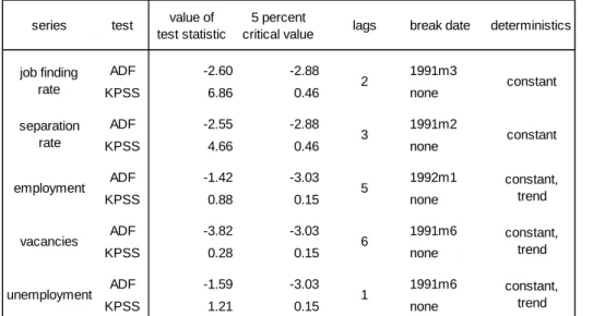
Table 1: Unit root tests
Note: ADF critical values according to Lanne et al. (2002), KPSS critical values according to Kwiatkowski et al.
(1992), KPSS test on reunification adjusted series.
KPSS rejects the null of stationarity for all series, and ADF does not reject the null of nonstationarity but for vacancies. We will allow for stochastic trends in all variables.
Vacancies might be a borderline case, but here the estimate of the trend variance could still become zero in our unobserved components framework.
4 In contrast to many other countries there are official monthly time series for the stock of voluntarily reported vacancies in Germany. This is the best approximation we can use. The series of total vacancies from the representative German job vacancy survey (Kettner et al. 2011) is too short and of too low frequency.
Corrections such as the relation of inflows of registered vacancies to all hires (Franz 2006, p. 106) do not consider structural or business cycle specialties of the vacancy reporting rate.
series test value of test statistic
5 percent
critical value lags break date deterministics
ADF -2.60 -2.88 1991m3
KPSS 6.86 0.46 none
ADF -2.55 -2.88 1991m2
KPSS 4.66 0.46 none
ADF -1.42 -3.03 1992m1
KPSS 0.88 0.15 none
ADF -3.82 -3.03 1991m6
KPSS 0.28 0.15 none
ADF -1.59 -3.03 1991m6
KPSS 1.21 0.15 none
constant, trend 1
job finding rate separation
rate
employment
vacancies
unemployment
5 constant,
trend constant,
trend 6
2 constant
3 constant
7 Results
7.1 States, innovations, and Beveridge curve dynamics
Correlated unobserved components models provide a very flexible framework without any a priori restrictions. Thus, they allow for a wide range of results that could not even
theoretically be achieved by more restrictive procedures. Within that range of results, two are frequently confirmed by the data: (1) a high negative correlation between trend and cycle of the decomposed series and (2) a trend component that is more volatile than the observed series itself (e. g. Morley et al. 2003, Sinclair 2009). This second feature is found for the unobserved components of matching efficiency, separation rate, and tightness (Figures 3 to 5).5 It reflects the multitude of shocks that cause persistent effects on the labour market. Also, it stands in contrast to the smooth trends resulting from standard – but also restrictive – filters like HP. Our results will lead us to a new perspective on the nature of movements along and shifts of the BC. Summarizing the co- or countermovement of the trends and cycles, we can conclude on permanent or transitory dynamics of the German BC, especially after the Hartz reforms.
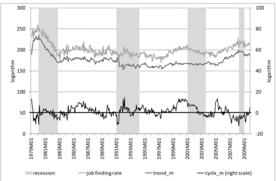
Figure 3 displays the job finding rate as well as trend and cycle of matching efficiency as estimated within the extended matching function.6 In the aftermath of the Hartz reforms, starting in 2003 and even more remarkably from 2005 on, the job finding rate increased considerably. The main reason for this improvement is an increase in matching efficiency which strongly supports empirical studies that state such a positive impact of the labour market reforms (Fahr/Sunde 2009, Klinger/Rothe 2012, Sala et al. 2013, Hertweck/Sigrist 2012). Our analysis moreover reveals that the increase took place in the permanent
5 Further results on variables not discussed in this section but included in the complete model specification are available from the authors on request.
6 Note that the trend constantly lies below the observed series due to the additional terms U and V on the right hand side of the matching function in equation (5).
component, in other words: labour market improvement after the reforms via matching efficiency was “structural”, indeed. A similar increase has never been observed before in the past 30 years. This is contrary to the economic upswing around the turn of the millennium, when the increase in the job finding rate was only temporary as the cyclical component rose while the trend stayed flat. Furthermore, the Great Recession at the turn of the years
2008/2009 did not lead to a sharp cyclical reaction but seems to mark the fading out of previous structural effects on matching efficiency.
Figure 3: Job finding rate and matching efficiency: observations, trend and cycle
Source: Institute for Employment Research and own estimation. Business cycle dating by ECRI.
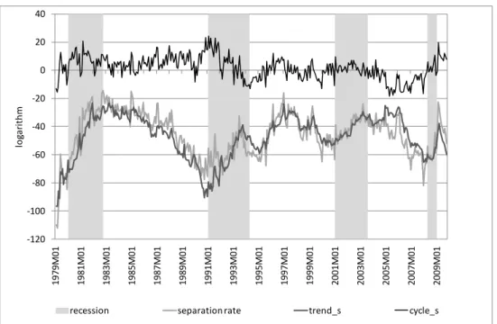
The separation rate plays a complementary role in explaining the BC´s inward shift after the labour market reforms. Its development is substantially driven by the trend (Figure 4);
increases during GDP recessions and decreases during GDP expansions were often caused by permanent shocks. After the labour market reforms, both trend and cycle caused the
separation rate to decrease, with the trend playing the major role. However, compared to historical developments, that trend decrease was not as outstanding as the jump in trend matching efficiency.
-20 0 20 40 60 80 100
0 50 100 150 200 250 300
1979M01 1981M01 1983M01 1985M01 1987M01 1989M01 1991M01 1993M01 1995M01 1997M01 1999M01 2001M01 2003M01 2005M01 2007M01 2009M01 logarithm
logarithm
recession job finding rate trend_m cycle_m (right scale)
Figure 4: Separation rate: observations, trend and cycle
Source: Institute for Employment Research and own estimation. Business cycle dating by ECRI.
Matching efficiency and separation rate determine the intercept of the BC with different signs.
In principle, they could compensate each other. But if they develop in opposite directions, as in the aftermath of the reforms, they strengthen each other´s effect on the shift of the BC.
In summary, the only inward shift of the German BC in the past 30 years took place mostly because the separation rate shrank and matching efficiency increased outstandingly, both for permanent reasons. Even though our analysis does not allow for a causal interpretation, this finding is a strong indicator for the effectiveness of the labour market reforms targeting exactly search effort and demand incentives. Economically, trend unemployment (compare equation (7)) shrank by 1.4 percent per month between its highest value in March 2005 and its lowest value in November 2008. The increase of trend matching efficiency and the decrease in trend separation rate each account for about half of that reduction (average growth
contribution -0.72 and -0.76 percentage points), whereas the influences of employment and vacancies were negligible at that time. Furthermore, we calculate average monthly changes for economic expansion years 1999/2000 and 2006-2008 when the remarkable BC inward shift took place. In the first phase, log trend unemployment shrank by 0.7 per month on
-120 -100 -80 -60 -40 -20 0 20 40
1979M01 1981M01 1983M01 1985M01 1987M01 1989M01 1991M01 1993M01 1995M01 1997M01 1999M01 2001M01 2003M01 2005M01 2007M01 2009M01
logarithm
recession separation rate trend_s cycle_s
average, in the second phase the monthly reduction was 1.2. The role of trend matching efficiency changes in these reductions increased from 31.8 percent in the first phase to 56.3 percent in the second phase while the importance of trend separation rate changes decreased from 94.1 to 58.8 percent.
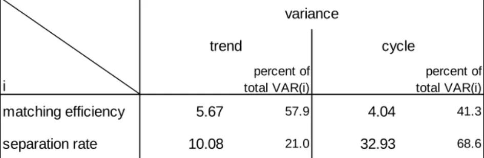
Considering the whole time span, the separation rate experienced more volatility and higher amplitudes than matching efficiency. After the early 1980s, BC shifts to the right were mainly caused by further increases in the structural separation rate whereas matching efficiency experienced rather limited changes. This connects to the studies by Fujita/Ramey (2009) or Hertweck/Sigrist (2012) that stress the importance of the separation rate for unemployment dynamics. This is proved by the variances of the shocks to trend and cycle separation rate that are much larger than those of the matching efficiency shocks (Table 2). Furthermore, the trend shock and the cycle shock of matching efficiency have similar variances whereas for the separation rate, the cycle shock variance is three times as large as the trend shock variance.
Table 2: Trend and cycle shock variances of matching efficiency and separation rate
Note: variance proportions of tightness larger than 100 because of negative covariance between trend and cycle.
It might appear puzzling that the shift of the BC became visible only in late 2006 although the shifting parameters already started to change in 2005. A similar seeming contradiction occurs in the early 1980s when the development of the BC may well be misinterpreted as movement along the curve although separation rate and matching efficiency changed tremendously. We can dissolve the conflict when considering the overlay of shifts on the one hand and
movements along the curve caused by – permanent or transitory – rotations of the job creation
percent of total VAR(i)
percent of total VAR(i)
matching efficiency 5.67 57.9 4.04 41.3
separation rate 10.08 21.0 32.93 68.6
i
variance
trend cycle
2s2m2E
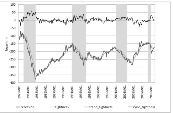
curve on the other. Notably, rotations of the job creation curve are reflected by changes in labour market tightness (compare Figure 2 in section 2). As Figure 5 shows, the trend of tightness is more volatile than the series calculated from the actual data. It also has a higher variance than the cycle. Consequently, rotations of the JCC occur mostly for permanent reasons. This is in line with business cycles driven by permanent productivity shocks (Morley et al. 2003, Weber 2011) and with the fact that structural change (sectors, technology) may come along with business cycle fluctuations (e. g. Caballero/Hammour 1994). The series of tightness adjusts sluggishly to trend shocks. This pattern creates a cycle with opposite sign during the time of adjustment (Morley et al. 2003) and implies a negative correlation between trend and cycle of tightness (see 7.2).
Figure 5: Tightness: observations, trend and cycle
Source: Federal Employment Agency and own estimation. Business cycle dating by ECRI.
Taking the development of trend matching efficiency, trend separation rate and trend tightness together, it becomes obvious that the steep increase in tightness after 2005 retarded the
appearance of the BC inward shift until tightness had reached its new persistent plateau.
Tightness rose so sharply because vacancies reacted quickly to the change in economic
-400 -350 -300 -250 -200 -150 -100 -50 0 50 100
1979M01 1981M01 1983M01 1985M01 1987M01 1989M01 1991M01 1993M01 1995M01 1997M01 1999M01 2001M01 2003M01 2005M01 2007M01 2009M01
logarithm
recession tightness trend_tightness cycle_tightness
conditions whereas it took unemployment some time to adjust to the new institutional framework. Besides this, deregulation in some segments led to an increase in demand for highly flexible labour such as short-term, fixed-term, part-time or temporary agency work. An increase in these kinds of jobs may inflate vacancies by a high turnover but not equivalently reduce unemployment. The slow adjustment of unemployment is confirmed by a negative correlation between its trend and cycle. By the same token, the flat downward slope of the BC in the early 1980s actually reflects permanent shifts to the right and movements down the curve at the same time.7
7.2 Correlations and labour market implications
The complex interactions on the labour market are elucidated by the several trend and cycle shocks correlations. Because of sluggish adjustment of time series to permanent shocks, most unobserved components studies estimate a negative correlation between trend and cycle of one and the same variable. In our application, this is only true for tightness whereas matching efficiency and separation rate show up with hardly any correlation between their trend and cycle shocks (Table 3). This accounts either for a very quick adjustment of the shifting parameters to changes in their trends or – which is more plausible with regard to the multiple sources of correlations in our multivariate model – for compensatory effects.
Table 3: Correlations between the shocks of the main unobserved states
7 Similarly, Fujita (2011) argues that increases in unemployment and drops in vacancies (movements along the curve, at first glance) come along with changes in separation rate and job finding rate – determinants of the intercept – as well as a hump-shaped vacancy development.
Matching efficiency and separation rate are negatively correlated in trends (-0.4) as well as in cycles (-1.0). With regard to the permanent components this correlation reveals that
institutional and structural change (or permanent productivity shocks) work through both channels in a similar way: the BC relocates through both shifting parameters into the same direction; the effects usually do not compensate each other, as would have been the case with positive correlation. Moreover, the two parameters follow an opposite cyclical pattern.
Trend separation rate and cyclical matching efficiency are correlated at 0.5 which suggests a time-consuming structural adjustment process on the labour market that is transitorily hidden by cyclical patterns. For example, when trend separations shrank in the aftermath of the reforms because labour demand increased and firms kept more of their staff, the pool of the unemployed does not get filled with just came-in unemployed that have good chances to leave quickly. As a result, matching efficiency shrinks, too, but only temporarily. In the long-run, instead, higher labour demand and the higher value of vacancies urges firms to search more intensively and hire people, which in the end raises permanent matching efficiency (see negative correlation above).
The correlations between the shifting parameters and tightness emphasize the overlay of shifts and movements along the curve, which was carved out in the previous subsection. The
correlations between trend tightness and trend matching efficiency at 0.6 as well as trend separation rate at -0.5 imply a permanent inward shift being accompanied by a permanent movement up the curve or vice versa. Exactly this was observed after the reforms.
trend_m trend_s trend_θ cycle_m cycle_s cycle_θ
trend_m 1 -0.42 0.55 0.01 -0.12 -0.42
trend_s 1 -0.53 0.52 0.14 0.62
trend_θ 1 0.40 -0.11 -0.82
cycle_m 1 -1.00 -0.68
cycle_s 1 0.18
cycle_θ 1
Economically, this can be explained by a common dependence of separations, vacancies, and unemployment on permanent changes of labour market institutions and productivity. Labour market institutions that change trend matching efficiency correspondingly change tightness as they influence vacancies via search costs and benefits of companies and unemployment via its duration.
7.3 The matching function
As announced in section 4, our model contains an extended matching function that may unfold different elasticities of matches with respect to the trends or cycles of unemployment and vacancies, an issue not considered in the literature so far. This section presents the
extended function, parameter estimates and interpretation. Equation (11) repeats the matching function with special regard to the unobserved components of unemployment and vacancies.
(11)
t
V t c V t U t c U t m
t m t
t c c c w
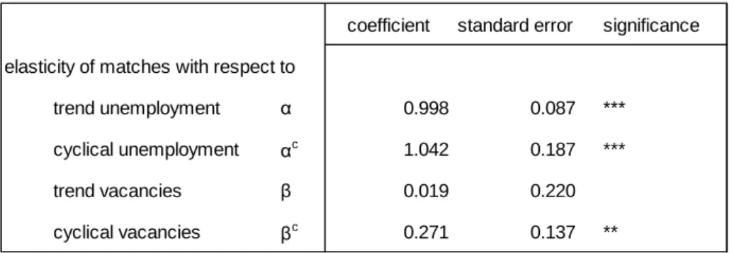
f 1 1 1 1 1 1 Parameter estimates are given in Table 4.
Table 4: Estimation results for the matching function
Significance levels: *** 1 percent, ** 5 percent.
Regarding unemployment, the generalization does not reveal different conclusions. The elasticities of matches with respect to both trend and cyclical unemployment are estimated at nearly 1 which is high compared to the summaries by Petrongolo/Pissarides (2001) or
Broersma/van Ours (1999). However, since we allowed for time-varying matching efficiency in our function, results are not directly comparable. Economically, an elasticity substantially
coefficient standard error significance elasticity of matches with respect to
trend unemployment α 0.998 0.087 ***
cyclical unemployment αc 1.042 0.187 ***
trend vacancies β 0.019 0.220
cyclical vacancies βc 0.271 0.137 **
smaller than 1 implies a disproportionately smaller reduction in matches when unemployment shrinks. This may not be plausible as a reduction in unemployment typically keeps merely bad risks within the pool. Matching function estimates for the group of the long-term unemployed by Klinger/Rothe (2012) came up with a very robust elasticity between 0.9 and 1, too.
In contrast to unemployment, the impact of vacancies in the extended matching function differs considerably between trend and cycle: trend vacancies are not significant; it is only the elasticity of matches with respect to cyclical vacancies that shows up with a significant
coefficient of 0.3. 8 This result resembles estimates of aggregate stock-flow matching functions that were rationalized by a systematic element in search (Coles/Smith 1998, Gregg/Petrongolo 2005, Fahr/Sunde 2009): unemployed already know the existing stock of vacancies but did not match. In the next round of applications, they will focus on newly incoming vacancies. Even though some people that just entered unemployment may match with old vacancies, this effect is not large enough to create a significant contribution of the stock of vacancies in the matching function.9 As these vacancies do not merge into matches, they become persistent and form at least part of the permanent component. Instead, inflows into vacancies have a significant impact with an elasticity usually estimated between 0.3 and 0.4. Those new vacancies are filled more easily, raise matches and, consequently, disappear – they are transitory. Given that such a procedure does not only refer to inflows but also holds for a proportion of our stock variable, this proportion of very short-term vacancies is likely to be part of our cyclical component.
8 In sum, our matching function then reveals slightly increasing returns to scale. Petrongolo/Pissarides (2001) also summarize studies that reject the null of constant returns. They argue as theoretical disadvantage, however, that increasing returns to scale are compatible with more than one equilibrium, one with high and one with low search activity.
9 Incidentally, this implies an elasticity of 1 for the stock of unemployment in constant returns to scale specifications as in Gregg/Petrongolo (2005).
8 Conclusions
The picture of the German BC between 1979 and 2009 shows movements along the curve with changing slope as well as many outward and one inward shift. As a reduced-form relationship, it reveals no insights into the drivers of these dynamics. Structural content is added to these descriptions by means of an unobserved components analysis, further considering cointegration between labour market variables. It disentangles each of the BC constituents into a permanent and a transitory series and allows analysing the time-varying properties of matching efficiency, separation rate, and tightness. Thereby, we gather information on the determinants of shifts of the BC, movements along the curve, and their interaction. This is especially valuable as the BC shifted inwards for the first time in decades after severe labour market reforms had come into force between 2003 and 2005. Thus, our analysis contributes to the macro-evaluation of that reform.
The inspection revealed the following main results: First, although the separation rate used to be the more pronounced factor in explaining BC dynamics over the whole time span, both separation rate and matching efficiency almost equally led to the inward shift after the reforms.
Second, the functioning of the labour market improved permanently, that is for structural reasons. The trend-cycle decomposition reveals an extraordinarily strong increase in trend matching efficiency which is in line with the aim of the Hartz reform to raise incentives for more intense job search as well as higher labour demand. The trend increase came to an end at the onset of the Great Recession.
Third, shifts as well as movements along the curve occur for permanent and transitory
reasons, usually at the same time. Thus, a sharp increase in trend tightness retarded the inward shift of the BC despite labour market functioning started to improve earlier.