Regensburger DISKUSSIONSBEITRÄGE zur Wirtschaftswissenschaft

(1)

Regensburger

DISKUSSIONSBEITRÄGE zur Wirtschaftswissenschaft

University of Regensburg Working Papers in Business, Economics and Management Information Systems

Your very private job agency: Job referrals based on residential location networks

Franziska Hawranek

^

and Norbert Schanne

^**

18.02.2015

Nr. 483

JEL Classification: C 31; D 83; E 24; J64

Key Words: Job referrals, Labor market, Neighborhood effects, Network effects, Social interactions

 Franziska Hawranek is a research assistant at the Department of Economics, Faculty of Business, Economics and Management Information Systems at the University of Regensburg, 93040 Regensburg, Germany

Phone: +49-941-943-5688, E-mail: franziska.hawranek@ur.de

** Norbert Schanne is a Senior Researcher at the Institute of Employment Research (IAB), Regional Research

(2)

Your very private job agency: Job referrals based on residential location networks

Franziska Hawranek^a,∗, Norbert Schanne^b

aUniversity of Regensburg, Universit¨atsstr. 31, 93053 Regensburg. Phone +49 941 943 5688

bInstitute for Employment Research (IAB), Regional Research Network IAB Hesse, Saonestr. 2-4, Frankfurt am Main, Germany. Phone +49 69 6670 519, Fax +49 69 6670

499

Abstract

This paper analyzes job referral effects that are based on residential location.

We use geo-referenced record data for the entire working population (liable to social security) and the corresponding establishments in the Rhine-Ruhr metropolitan area, which is Germany’s largest metropolitan area. We estimate the propensity of two persons to work at the same place when residing in the same neighborhood (reported with an accuracy of 500m×500m grid cells), and compare the effect to people living in adjacent neighborhoods. We find a significant increase in the probability of working together when living in the same neighborhood, which is stable across various specifications. We differentiate these referral effects for socioeconomic groups and find especially strong effects for migrant groups from former guest-worker countries and new EU countries.

Further, we are able to investigate a number of issues in order to deepen the insight on actual job referrals: distinguishing between the effects on working in the same neighborhood and working in the same establishment – probably the more accurate measure for job referrals – shows that the latter yield larger relative effects. Besides, we find that clusters in employment although having a significant positive effect play only a minor role for the magnitude of the referral effect. We find evidence that informal job markets play the biggest role in small firms and are least important in large firms. When we exclude short distance commuters, we find the same probabilities of working together, which reinforces our interpretation of this probability as a network effect.

Keywords: Job referrals, Labor market, Neighborhood effects, Network effects, Social interactions

∗Corresponding author

Email addresses: franziska.hawranek@ur.de(Franziska Hawranek), norbert.schanne@iab.de(Norbert Schanne)

(3)

1. Introduction

In social sciences the interest of interactions between individuals has increased: how do people influence one another and how can we measure this interaction? In labor economics, the importance of social interactions for the determination of labor market outcomes has drawn attention in the last years.

One aspect of social interactions is interaction on a very local level: how does sharing a residential neighborhood (and therefore facing the same institutions and infrastructure) affect labor market outcomes? The channels hereby can be diverse including e.g. spatial mismatch (Kain, 1968), discrimination, differences in access to resources (such as education, B´enabou (1994)) or differences in at- titudes and role models across neighborhoods (Jencks and Mayer, 1990). In this paper, we look at how residential neighborhoods can serve as a pool of information for an informal labor market and investigate the effect of job referrals through one’s residential location.

In particular, we analyze the relationship between living and working together in the context of job referrals in the Rhine-Ruhr metropolitan area. The Rhine- Ruhr is Germany’s largest and the EU’s second largest agglomeration, located in North Rhine-Westphalia. It is spread across 7,110 km² including big cities like Cologne, D¨usseldorf and Dortmund. The metropolitan area is home to over 11 million inhabitants and is especially interesting for urban analysis due to its densely populated nature and the economic diversity.¹

Our empirical framework is possible due to a novel data set covering geo-coded record data for the entire working population (liable to social security) and the corresponding establishments. As social interaction is not measurable directly with any kind of administrative data, we use a well-established approach to ap- proximate a local network effect: We estimate the propensity of two individuals to work at the same place when residing in the same neighborhood (reported with an accuracy of 500m×500m grid cells) with a linear probability model (LPM), and compare it to the propensity of two individuals residing in adjacent neighborhoods, conditional on a super-neighborhood fixed effect (where super- neighborhoods are all adjacent neighborhood grid cells). The empirical design follows Bayer et al. (2008).² We find very similar effects: Bayer et al. (2008) estimate that sharing the same immediate neighborhood raises the propensity

1Traditionally, the Rhine-Ruhr was specialized in heavy industry and mining. The struc- tural change in the 1960s lead to a specialization in the service sector. Until today, the area is economically contrasting with high unemployment rates in Dortmund and Gelsenkirchen on the one hand and the prospering Rhine area on the other hand. See figure A.3 in the Appendix.

2Bayer et al. (2008) use Census data for the Boston metropolitan area, which has 4.5 million inhabitants and is spread over 12,105km².

(4)

to work together by 0.12 percentage points, whereas the effect is 0.14 percentage points in our case. This translates into a relative increase in the probability of working in the same neighborhood of 8%. When analyzing the effect of working in the same firm we even find an increase in probability of about 30%.

We rule out several alternative explanations for this propensity effect,in particular a reverse direction of housing referrals amongst colleagues and the spurious arising of correlation due to the geography of workplaces and transportation infrastructure, by conducting a number of robustness checks. This makes us confident to interpret this effect as an indication for a job referral where information on an informal job market is circulated in one’s residential neighborhood.

To examine how different groups of workers make use of informal networks, we differentiate job referral effects by characteristics such as education, industry, nationality or age groups. The effects differ especially by ethnicity: compared to Germans, the propensity to work together when sharing the same neighborhood is highly increased, in particular for immigrants from new EU countries but also from the former guest-worker countries Spain and Italy.

To this point, we cannot say anything about who (within a pair) benefits from this local effect on one’s information set but focus on identifying the exist- ence and credibility of a residential referral effect. Our network effect clearly is an approximation for network activity and as presumably other forms of networks exist in an informal job market. The literature distinguishes three types of informal job market networks: networks of former colleagues or classmates (see e.g. Glitz (2013), Dustmann et al. (2011), Kramarz and Nordstr¨om Skans (2013), Marmaros and Sacerdote (2002) and Saygin et al. (2014)), family networks (see e.g. Kramarz and Nordstr¨om Skans (2013)), and residence based networks (see e.g. Bayer et al. (2008), Schmutte (2014), Hellerstein et al. (2011)).

We show that residence based networks play an important role, especially for low skilled and minority workers. Moreover, the effect of residence based networks can have important implications for spatially based policies: if networks for an informal job market exist in residential locations, they can potentially be used for unemployment policies and generate local spill overs.

The goal of this paper is first to look at how referral effects based on residential location may differ for a European country as opposed to US American data, given that institutional backgrounds and cultural conventions are quite different with respect to the labor market and job search. In addition, we are able to investigate a number of issues in order to shed further light on actual job referral effects: First, our data allows us to distinguish between the effects on working in the same neighborhood and working in the same establishment - probably the more accurate measure for job referrals. Second, an advantage of the data set we use is the overlapping structure of our reference groups, the so-

(5)

called super-neighborhoods. A crucial assumption for the identification of social interaction is that there is no sorting by unobservables within these reference groups. When conditioning on a fixed reference group as in Bayer et al. (2008) or Schmutte (2014), this assumption is less likely to hold as when using a rolling window design. Third, we analyze to what extent the findings are due to highly concentrated clusters of employment opportunities in central business districts, and find small positive bias in the referral to a neighborhood. Finally, we address to what extent people tend to work in their residential neighborhood, and whether the evidence in the literature is affected by inadequately accounting for short-distance commuting behavior. In contrast to previous work, we also incorporate data on commuting networks and find them not to be the driver of our measured interaction effect.

The remainder of the paper is structured as follows. Section 2 gives an overview on the related literature. Section 3 describes the data set we use for the Ger- man Rhine-Ruhr area. Section 4 presents the research design and the baseline model. In section 5 we discuss our results as well as robustness checks and further specifications. Section 7 concludes.

2. Literature Review

In this paper, we focus on social interactions in the form of network effects on an informal job market. As Montgomery (1991) points out, there is asym- metric information on the labor market. Employers cannot observe applicants’

true productivity, such that they have an incentive to rely on referrals from their own employees to reduce search costs and avoid adverse selection. Additionally, Topa (2001) shows that workers have an incentive to share information on avail- able jobs with their network while being employed, as this information sharing serves as an insurance for the state of unemployment. Hence, in equilibrium one should observe assortative matching of employees with their social networks. ? suggest, that one natural form of such a network for information exchange is the physically proximate space surrounding individuals, such as residential neighborhoods. Neighborhoods qualify as information transmission environments, because of the low transportation costs within neighborhoods (both monetary and time costs) and because of local institutions, where people can meet and interact, such as schools, churches or clubs. The work most related to ours is Bayer et al. (2008), who also estimate the propensity of working together, when living in the same as opposed to a nearby neighborhood. They use the 1990 U.S. Census of Population for the Boston metropolitan area and define census blocks as neighborhoods and census block groups as super-neighborhoods. We choose this paper as a point of departure, as the authors make a strong case

(6)

for identifying social interaction in a very specific way, given the assumption of no correlation in unobservables within super-neighborhoods. In contrast to Bayer et al. (2008), our data provides information on the exact establishments of workers. This specification reflects a referral effect much more realistically.

First, because theory as in Montgomery (1991) suggests that employers have an incentive to hire workers’ social contacts, which is why we would expect to observe workers from the same network at a firm level. Second, it is more likely that workers gather information on job openings in their own establishment rather than in the firm’s neighborhood.

Numerous other papers emphasize the importance of informal job markets like Ioannides and Datcher Loury (2004) and Corcoran et al. (1980) using US data.

Glitz (2013) and Dustmann et al. (2011) investigate the effects of coworker networks on labor market outcomes using German and Saygin et al. (2014) using Austrian record data. Glitz (2013) finds strong positive effects on own probability of working and wages, which indicates significant effects of social networks in the German labor force on labor market outcomes.

Ioannides and Datcher Loury (2004) summarize stylized facts on the usage of informal job search channels. About 15% of unemployed Americans use friends and acquaintances for job search.³ They report variation in the usage of such information channels among age and socioeconomic groups: e.g. woman and individuals with better education use friends and family less often whereas the findings for older people are opposing.⁴ Kramarz and Nordstr¨om Skans (2013) analyze how networks of families affect labor market outcomes. Following Gran- ovetter (1973), they distinguish between how strong ties, namely family and weak ties like classmates and neighbors affect the decisions of youths in Sweden⁵ who enter the labor market. They find that the effect of strong ties is important, but only significant if one parent is currently employed at the same plant. The effect is stronger for low educated youths, those with bad grades or bad training and for immigrants.

Pellizziari (2010) shows⁶that about 30% of Germans use personal contacts for finding a job whereas only about 15% of US Americans use such search chan-

3Using the PSID 1993, Ioannides and Datcher Loury (2004) find that 15.5 percent of unemployed and 8.5 percent of employed ask friends and relatives about potential job openings.

4Ports (1993) find increased usage of informal channels for 45-55 year-olds and 55-65 year- olds in 1992 respectively analyzing CPS data. On the contrary, e.g. Corcoran et al. (1980) report that usage of informal job market declines with age and/or work experience. Holzer (1987) finds that especially young people aged 16 to 23 rely on friends and relatives in 60-70%

of all jobs they actually attained (using data on search methods from the 1981 NLSY).

5They analyze this question using a population wide data set linking graduation records and family ties to longitudinal matched employer-employee data with information on the firms.

6The author uses the European Community Household Panel (ECHP) from 1994-2001 and the NLSY from 1979-2000

(7)

nels. This suggests that job referrals might play an even more important role in European countries as compared to in the US⁷.

Hellerstein et al. (2011) test for the presence and importance of residential networks (defined by census tracts) to determine the assignment of workers to establishments. They use a measure of workplace segregation by residential ori- gin and compare this to the share of co-workers that would come from the same neighborhood if workplaces were randomly assigned. They find a significant role of residence based networks using US 2000 Decennial Employer-Employee Database (DEED), which is especially strong for unskilled workers, minorities and workers in small establishments. Using a similar method and the same data, Hellerstein et al. (2014) investigate the outcome of residence-based labor market networks. They find a positive earnings effects and a lower turnover for workers more connected to their neighbors, especially if neighbors have the same race and hence interpret their results as evidence for productivity enhancing spillovers.

Schmutte (2014) also studies the effects of residence based networks on labor market outcomes like earnings. Identifying local interaction with the design of Bayer et al. (2008) as a first stage, he uses LEHD US employer-employee data to estimate an employer-specific wage premium. He finds that workers living in a neighborhood with high-quality networks are more likely to move to a better paying job. In particular, a one standard deviation increase in network quality is associated with a 25% increase in firm-specific wage premium on job change.

Overall, the evidence suggests that referral effects may differ between socioeconomic characteristics, which is why we will differentiate between industries, age groups, nationality and education categories.

3. Data

In this study we employ register data which are collected in the administrative processes of the German Federal Employment Agency (FEA, Bundesagentur f¨ur Arbeit) and maintained in the Integrated Employment Biographies (IEB) of the Institute of Employment Research (Institut f¨ur Arbeitsmarkt- und Berufs- forschung, IAB). The IEB cover all employed persons who pay statutory social security contributions, all recipients of benefits from unemployment security (according to Social Code III) or from basic life support (according to Social Code II), all participants in active labor market policy, as well as all persons who approach FEA for job-search support. Due to the parallel nature of the various data bases stemming from different processes, multiple spells may coex- ist for each person at the same time (e.g. because a person searches for a new

7The difference in data sources limits the exact comparability of these numbers.

(8)

job while being employed). If existing, the employment spell with the highest salary is defined as themain spell.

To ease computation we use data only for the Rhine-Ruhr region, Germany’s largest metropolitan area. It is a very densely populated area reflecting several aspects that also represent the whole of Germany. The area is diverse in its wealth and socioeconomic structure. It includes on the one hand prospering university cities like Bonn and on the other hand former heavy industry and mining centers, which have a high population of immigrants and also a high proportion of unemployment like Gelsenkirchen. The IAB Research Data Centre geo-coded both the work-place and the residential address corresponding to each person’s main spell at June 30th 2008 (see Scholz et al. (2012)). Each person is assigned to a quadratic grid cell of 500m length to warrant anonymity compulsory in social security data provision. We use these grid cells as our basic definition of a neighborhood.

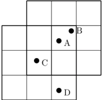
uC

uD uA

uB

Figure 1: Defining neighborhood by a regular grid

Figure 1 shows the structure of the neighborhood definition: According to the exact address, every individual is assigned to a grid cell (the small squares correspond to 500m×500m grid cells). Individuals A and B are immediate neighbors here, whereas C shares what we will further on call “super-neighborhood”

with A and B. D lives within a super-neighborhood of C but not with A and B.

In contrast to Bayer et al. (2008) who use predefined census blocks (neighborhoods) which belong to a fixed census block group (super-neighborhood), every grid cell (neighborhood) in our design is the centroid of a super-neighborhood and thus every grid cell belongs to several super-neighborhoods. Although the classification of neighborhoods and super-neighborhoods does not depend on geographic factors such as big roads or rivers, the flexible design guarantees an assignment for each grid cell to be the centroid of a super-neighborhood as well as part of the surrounding for all neighboring grid cells. We believe that this overlapping sampling scheme is an advantage as measured interaction is still

(9)

very local but the conditioning surrounding is flexible.⁸ It may frequently hap- pen that a person resides close to the outside border of the super-neighborhood when using a fixed definition as in Bayer et al. (2008). This can lead to scenarios, where the adjacent reference group or super-neighborhood would be closer to a person than the actual reference group the estimation strategy is conditioning on⁹ We use super-neighborhood fixed effects to deal with sorting on the basis of unobservables. As every grid cell belongs to 9 different super-neighborhoods, the influence of the remaining sorting within super-neighborhoods should be reduced substantially. Besides, using a neighborhood definition that is based on real distances rather than the number of people sharing a neighborhood (as it is the case for census blocks and census block groups) makes accounting for distances to workplaces and reflecting commuting behavior more realistic.

Within the geocoded IEB for Rhine-Ruhr, we observe roughly 4 million persons, dispersed across 21,509 grid cells, who are aged 15-65 and participate in the labor force (without self-employed, civil servants and members of the armed forces). Of these persons, roughly 3.5 million persons are employees. To get a file with individual data that is feasible for computation, we draw a 2% random sample from all employed persons and will further denote these individuals as i. They are combined with all persons residing within their own neighborhood or in one of the eight contiguous neighborhoods; we denote all possible neighbors asj and will further analyze pairsij, who reside in the same super- neighborhood. Compared to working with (possibly larger) samples for both individuals and neighbors, the one-sided sampling has the advantage to enable conclusions on job referrals in the population more easily (with one-dimensional sampling probabilities, respectively univariate rather than bivariate cumulated densities). All in all, we observe approximately 3.4 million persons living in one of the super-neighborhoods. Figure A.4 in the appendix shows the distribution of neighborhood and super-neighborhood sizes. The mass of the neighborhood- size distribution lies in the range between 150 and 700 persons per grid cell; the average neighborhood size is around 320. However, the average pair is observed in a neighborhood with more than 900 inhabitants because larger neighborhoods have a higher probability to be represented in the sample, and a person in a large neighborhood has more neighbors.

The geographic scale in the IEB data set differs from that in the role model paper. While Bayer et al. (2008) use census blocks (which on average measure

8This kind of mutually non-exclusive rolling-window delineation of super-neighborhoods is also a method of identifying neighborhood effects (Bramoull´e et al., 2009).

9If we would consider only the lower block of grid cells in figure 1 as a fixed reference group, e.g. individual B would have D in its reference group, but none in the adjacent grid cells on its right or above.

(10)

Legend

Municipalities Employment per grid cell

20 - 118 119 - 245 246 - 387 388 - 552 553 - 794 795 - 1235 1236 - 2256

0 5 10 20 30

Kilometers

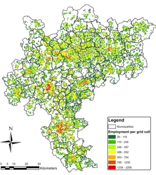
Figure 2: Employees in 500×500m grid cells in the Rhine-Ruhr metropolitan area

160m of length) as a definition for neighborhoods, our neighborhoods are considerably larger measuring 500m×500m. Nevertheless, we believe that this extent is small enough to guarantee the possibility of individuals actually interacting with each other. For example the edge length of a grid cell corresponds to the standard distance between bus stops for medium and highly populated urban areas (see K¨ohler and Bertocchi, 2010). It approximates a walking distance of five minutes. Social interaction in a residential neighborhood can occur through meeting at points such as sport clubs, churches or elementary schools¹⁰.

To illustrate the neighborhood sizes and the geographic extent of the data set,

10The whole Rhine-Ruhr area compasses 1,774 elementary schools, which differ in their dispersion: on the basis of municipalities (German “Kreise” and “kreisfreie St¨adte”), there is one elementary school per 2,522 inhabitants and a maximum 7,840 inhabitants per elementary school (data from the ministry of education in North Rhine-Westphalia at www.schulministerium.nrw.de). 2,522 inhabitants correspond to less than 1,100 employees when using the ratio of 35.9 Mio employees over 82 Mio inhabitants in Germany 2008 as an approximation. If we believe that e.g. parents meet when picking up their children and possibly form social contacts there, the extent of the draw area is larger than that of a residential neighborhood in our definition but smaller than a super-neighborhood.

(11)

figure 2 shows the dispersion of individuals in our sample in the Rhein-Ruhr area. Each dot represents a 500×500m grid cell and corresponds to our definition of a residential neighborhood. As figure 2 shows, the whole area is mostly densely populated. A comparison to figure A.3 in the appendix shows, that the most densely populated grid cells (the red areas) coincide with the area around Cologne in the South, D¨usseldorf in the West and Dortmund in the East.

In table 1 we compare groups in the population, in the sample, and in the neighborhoods and super-neighborhoods of the sampled persons. As table 1 shows, the 2% sample is almost identical to the population with respect to observable characteristics. The groups considered here correspond to the covariates in our estimations. The countries and groups of countries are the largest immigrant groups and those who traditionally came to Germany as guest-workers (southern European countries). Therefore we expect those groups to have formed particularly strong networks within Germany.

Table 1: Group sizes in population and sample

Group Population Sample Neighbors Super-neighbors

Male 0.5181 .5168 .5182 .5180

Age 15-24 0.0985 .0991 .0993 .0993

Age 25-34 0.2000 .2001 .2053 .2023

Age 35-54 0.5392 .5405 .5417 .5439

Age 55-65 0.1531 .1515 .1536 .1545

Unskilled 0.1485 .1477 .1509 .1493

Med. skilled 0.4750 .4780 .4722 .4752

Highskilled 0.0963 .0932 .0960 .0967

German 0.9032 .9018 .8992 .9023

Greek 0.0051 .0052 .0053 .0051

Italian 0.0086 .0083 .0089 .0086

Spanish 0.0019 .0021 .0020 .0020

Turkish 0.0352 .0355 .0372 .0357

Yugoslavian^a 0.0104 .0105 .0108 .0104

From new EU^a 0.0068 .0070 .0067 .0068

Other nationality 0.0288 .0296 .0298 .0290

Primary sector 0.0395 .0405 .0388 .0394

Manufacturing 0.1763 .1779 .1754 .1764

Construction 0.0458 .0455 .0455 .0457

TTC^b 0.2622 .2643 .2630 .2620

Business Services 0.1757 .1746 .1765 .1758

Other Services 0.3005 .2972 .3007 .3008

# employees 3,459,941 68,947 3,169,180 3,397,929

a: Yugoslavian covers immigrants from the territory of former Yugoslavia (including Slovenia and Croatia); these are not included in the group of immigrants from new EU members (which come from Estonia, Latvia, Lithuania, Poland, Czech Republic, Slovakia, Hungary, Bulgaria, Romania, Malta and Cyprus).

b: Trade, Transportation and Communication (TTC).

(12)

4. Empirical Design

Our goal is to compare the propensity of individuals working together for those living in the same neighborhood with individuals living close by. Our empirical design allows to identify a social interaction effect based on within super-neighborhood variation. The baseline model can be summarized as follows:

W_ijâ =ρs+α0Rⁿ_ij+εij witha= {n, f} (1) i and j denote individuals living in the same super-neighborhood (block of 9 grid cells, see figure 1) andW_ijâ is an indicator for both individuals sharing the same work place. W_ijâ takes on the values 0 or 100 so that parameters in the LPM directly represent changes in percentage points. We differentiateW_ijâ over a= {n, f}: first, we follow Bayer et al. (2008) and define the same work place as the neighborhood n where an individual works.¹¹ Second, we use exact information on the establishments, whereW_ij^f =100 if a pair of individuals works at the exact same firm. All specifications are estimated with heteroscedasticity and cluster robust standard errors¹². Rⁿ_ij is equal to 1 if bothi and j live in the same grid cell and zero otherwise. Therefore we can interpretα0, the social interaction effect, as the increase in probability of working together when sharing a neighborhood. ρs denotes a fixed effect for the super-neighborhood. It deals with sorting into residential location which leads to selection bias due to correlation in unobservable factors in neighborhoods (such as amenities or the access to public transportation), an important issue in the neighborhood effects literature. α₀can be identified as the social interaction effect given that the two key assumptions are fulfilled: First, social interaction within a neighborhood is a local phenomenon. Second, individuals are able to choose their residential location freely across super-neighborhoods but are randomly located within, such that there is no correlation in unobservable characteristics affecting both work place and residential location within a super-neighborhood.

To meet the requirement of the latter assumption, Bayer et al. (2008) argue that on a very local level, the housing market is comparably thin. When individuals are choosing their residential location, it may be hard to observe variation within super-neighborhoods, whereas it is easier to see this variation between

11A workplace area has size 1km×1km as to allow for more manufacturing establishments (which occupy more space than most services) to be in the same area.

12Following Angrist and Pischke (2009), including robust standard errors deals with most of the problems when applying an LPM. Additional to the more straight forward interpretation of LPM estimating e.g. a Probit model would make computation more difficult given the extent of the data set.

(13)

the larger super-neighborhoods. Furthermore, as with 500m length a neighborhood is considerably small, such that it is not necessarily the case that one can find a suitable dwelling given an appropriate search period in an exact small neighborhood, but rather has to look for something in a more spacious area (such as the super-neighborhood). Germans in general are less mobile compared to US Americans: 16% of Germans have changed their residence within the last two years and only 9% moved within a city (B¨oltken et al., 2013)¹³, which gives rise to the assumption that the thinness of the housing market is plausible even within cities. Besides, the overlapping structure of our super- neighborhood design should additionally contribute to meet this criterion: even if there is sorting within super-neighborhoods, sampling each small grid cell up to 9 times should substantially reduce the remaining sorting. This is a clear advantage as compared to Bayer et al. (2008) and Schmutte (2014), who use predefined fixed census block groups as a reference group.

To account for differences in the usage of informal networks between socioeconomic groups, we include individual characteristics.

W_ij^a =ρs+β^′(Xi−X¯) + (α0+α^′₁(Xi−X¯))Rⁿ_ij+εij witha= {n, f} (2) Here we can investigate how belonging to a certain group adds to the propensity of working together. α1depicts the effect of being part of a particular group and working together - a “one-sided” social interaction effect. To interpret the effect of sharing a neighborhood at the mean of the categorical variablesX, we center all covariates around zero.¹⁴ We use categorical variables for personal characteristics such as sex, age groups¹⁵, skill groups¹⁶, categories of nationality, different industries, and a control for the size of the neighborhood. β can be interpreted as the baseline propensity of residing in the same super-neighborhood (belonging to the same reference group) but not sharing an immediate neighborhood

13Bayer et al. (2008) argue, that only 11 percent of the owner occupants in their census sample had changed owners. As the data we use is registry data, we cannot observe how people live and have to rely on additional data for motivational reasons. In Germany, the owner occupancy rate is considerably smaller - about 50% (B¨oltken et al., 2013) - as compared to the US where the rate is about 70% (Ihrke and Faber, 2012). Both in Germany and the US, owner-occupants are less mobile: in the German data, only 6.3% moved in the last two years and only 3.6% moved within a city. As moving rates for Germans are comparably smaller anyway, we believe that the argumentation of Bayer et al. (2008) holds for our data set, too.

14Wooldridge (2002) argues that subtracting the sample mean from each component allows identification ofα0 as the average treatment effect ofRijon the dependent variable.

15Young adults from 15-24, career entrants aged 25-34, those established in the work force from 35-54 and senior workers between 55 and 65 years.

16Low skilled refers to lower secondary education with and without apprenticeship. Medium skilled individuals have higher secondary education (German “Abitur”), with and without apprenticeship. The high skilled group refers to individuals with a university degree.

(14)

on working together for different characteristic groups (X_i).

W_ij^a =ρ_s+β^′(X_ij−X) + (α¯ ₀+α^′₁(X_ij−X¯))R_ijⁿ +ε_ij witha= {n, f} (3) In equation 3, we examine whether the propensity of working together varies with the characteristics of a pair (as opposed to the individual characteristic measured by equation 2). Including this specification aims to investigate whether e.g. more similar pairs are more likely to profit from social interaction and whether certain groups have higher probabilities to work together, because of a stronger attachment to the labor market. Both equation 2 and 3 can be used to validate our estimates with evidence from the informal job market and network literature presented in section 2.

5. Results

Table 2 summarizes the results from our baseline model as presented in section 4. Estimating unconditionally (without super-neighborhood fixed effects) gives an impressions on the baseline probability of working together¹⁷: when residing in the same super-neighborhood the probability of working in the same neighborhood is 1.8% and 0.22% for working in the same firm. Estimating equa- tions 1-3 can then be interpreted as an increase in this baseline probability by residing in the same neighborhood.

Column (1) corresponds to equation 1, where sharing a neighborhood is the single explanatory variable. The social interaction effect is positive and highly significant for both cases ofa= (n, f), which means evidence for a positive impact of sharing a residential neighborhood on the propensity to work together.

For a referral to a neighborhood (a=n), the probability of working together is increased by 0.14 percentage points, which corresponds to an increase by 8%.

Despite the different definition of neighborhoods the magnitude of the social interaction effect is similar compared to the 0.12 percentage points estimated by Bayer et al. (2008).

Interpreting the referral to a firm can be seen as an even higher indication for an actual job referral. The estimated absolute social interaction effect is some- what smaller as compared to the referral to neighborhood effect, albeit still positive and highly significant. The probability to work together at the same firm increases by 0.07 percentage points if a pair of individuals lives in the same neighborhood. This is equivalent to a 30% increase in probability compared to the unconditional baseline probability which is much larger than in the case of a

17Here, we estimateW_ij^a=α0+α1Rⁿ_ij+εijand interpretα0 as the baseline probability of working together when sharing the same super-neighborhood.

(15)

Table2:EstimationofReferralEffects VariableReferraltoneighborhood(a=n)Referraltofirm(a=f) NoFE(1)(2)(3)NoFE(1)(2)(3) Constant1.7982∗∗∗ 1.7941∗∗∗ 2.2207∗∗∗ 2.0837∗∗∗ .2169∗∗∗ .2189∗∗∗ .2347∗∗∗ -.1196 (.0011)(.0037)(.4000)(.3811)(.0004)(.0038)(.1063)(.1054) Rij.1111∗∗∗ .1368∗∗∗ .1432∗∗∗ .1238∗∗∗ .0868∗∗∗ .0746∗∗∗ .0784∗∗∗ .0605∗∗∗ (.0027)(.0238)(.0238)(.0185)(.0010)(.0240)(.0241)(.0182) Relativeincrease[7.61%][7.96%][6.88%][34.39%][36.15%][27.89%] Sex––Xi∗∗∗Xij∗∗∗––Xi∗∗∗Xij∗∗∗ RijXiRijXij∗∗∗ RijXiRijXij∗∗∗ Qualification––Xi∗∗∗ Xij

∗∗∗ ––Xi

∗∗∗ Xij

∗∗∗ RijXiRijXij∗∗∗ RijXiRijXij∗∗∗ Agegroup––Xi∗∗∗ Xij

∗∗∗ ––Xi

∗∗∗ Xij

∗∗∗ RijXiRijXijRijXiRijXij∗∗∗ Ethnicity––Xi∗∗∗ Xij

∗∗∗ ––Xi

∗∗∗ Xij

∗∗∗ RijXi∗∗ RijXij∗∗∗ RijXi∗∗ RijXij∗∗∗ Industry––Xi∗∗∗ Xij∗∗∗ ––Xi∗∗∗ Xij∗∗∗ RijXi∗∗ RijXij

∗∗∗ RijXi

∗∗∗ RijXij

∗∗∗ lncoresize––XiXij––XiXij RijXi∗∗∗ RijXij

∗∗∗ RijXi

∗∗∗ RijXij

∗∗∗ σu–5.293436.679531.1610–2.53825.10424.6731 σε13.35113.288113.282113.27034.79564.76544.76234.7485 #pairs179.7Mio179.7Mio179.7Mio179.7Mio179.7Mio179.7Mio179.7Mio179.7Mio #groups–117571015910159–117571015910159 Corr(u,Xb)–-.0072-.0042-.9996–.0083.0249-.9984 Heteroscedasticity-consistentstandarderrorsinparentheses. ∗/∗∗/∗∗∗marksignificanceatthe90%/95%/99%confidencelevel. Asterisksatthecontrolvariablesandinteractiontermsmarksignificantdifferencesbetweenthegroups.ReferenceisafemaleGerman intheagebetween35and54withunknownqualificationworkinginManufacturing,orapairoftwowomenwiththesecharacteristics, respectively.Coefficientestimatesarereportedintheappendix.

(16)

referral to a neighborhood. This means that the case of(a=f)not only reflects an actual referral more realistically, but also is economically more meaningful.

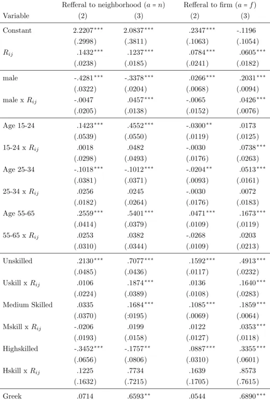
Columns (2) and (3) refer to equation 2 and equation 3, where we are inter- ested in how the social interaction effect reacts first for different socioeconomic groups and second for pairs of socioeconomic groups. For expositional purpose, we only report joint significance in this table; full outputs are presented in the appendix. Noticeably, the social interaction effectα0 is relatively stable across specifications. Column (2) shows the one-sided interaction effect. Here, only some of the interactions are jointly significant: there is no statistically significant differential effect of sharing a neighborhood varying by qualification, age group or gender both for referrals to neighborhoods and to firms. An individual’s own ethnicity¹⁸ and in which industry¹⁹ one works generate significant variation in the referral effect. The larger a neighborhoodilives in, the smaller the referral effect; this probably corresponds to the likelihood of interaction the more individuals reside in a neighborhood.

Column (3) describes how pairs of certain groups interact in residential neighborhoods. The effect of Xij describes the propensity to work together when sharing a super-neighborhood: as expected, we see higher propensities for young and old pairs of workers, as well as unskilled pairs and matches for several industry sectors, but almost no effect of ethnic groups. Again the interaction term determines the local referral effect. Apart from age groups, the impact of all categories are jointly significant which indicates that grouping pairs with respect to socioeconomic categories at least plays some role for job referrals. The interaction effects (α1in equation 3) can be interpreted as the additional effect of being both in the same socioeconomic group and sharing the same neighborhood. There are no big differences across gender and age groups (meaning that the interaction effects are either small or insignificant). Consistent with the literature on informal job markets, pairs of unskilled workers have a comparatively higher propensity to work together both at the same neighborhood and at the same firm. For different ethnic groups the effect varies, too: especially for people from the new EU countries, the probability to work together increases by over 20% as compared to Germans (the reference group) both for referrals to neighborhoods and referrals to firms. Also Italians and people from former Yugoslavia show stronger referral effects. In contrast, albeit being the

18The effect differs between referrals to neighborhoods, where Greeks have the most significant increase in probability of working together, and referrals to neighborhoods, where Turks seem to profit the most from referral effects. For all other groups, the effects are positive but rather noisy.

19Compared to women working in manufacturing, working in all other industry sectors has a negative effect on working together when sharing a neighborhood, with business related services having the largest and most significant effect.

(17)

biggest migrant group in Germany, Turkish do not seem to behave differently than Germans, with the interaction effect being insignificant. For the different types of industries²⁰, the propensity to work together is increased in a similar way across groups. The size of the residential neighborhood of pairs seems to have no effect on working together; it has a significant negative effect on the interaction (the referral), however. We interpret this as decreasing probability to meet when living in a higher populated neighborhood, a result also stated by Calv`o-Armengol and Zenou (2005)²¹.

We use a linear model for computational reasons. One concern on the specification could be that estimating a linear model does not accurately reflect potential non-linearities in the propensity of working together and therefore overstates the true network effect. We therefore calculate linear predictions of ˆWij using equation 2 and 3. We find mean and median predicted probability to be close to the baseline probability of working together in a super-neighborhood, which we interpret as an indication for an LPM being a correct specification.

6. Robustness and Discussion

The baseline model presented above has three major issues for identifying a causal social interaction effect: self selection, potential simultaneity bias, and spurious correlation due to geography. In the following, we discuss strategies to reduce these problems.

6.1. Sorting within super-neighborhoods

We want to make sure the key assumption for identification, no correlation in unobservables affecting work location within a super-neighborhood, can be re- garded as reasonable. Following Altonji et al. (2005), selectivity in observables is proportional to selectivity in unobservables and can be seen as an indication of sorting by unobservable characteristics. Therefore, we first analyze the sorting behavior with respect to observable characteristics. We compute correlations of observable characteristics (age groups, gender, nationality groups, skill groups and industry groups) E(Di 1

ni∑_jDj) =E(Xij)for both pairs that reside in a neighborhood together and for pairs who share a super-neighborhood but are not immediate neighbors²², and test whether they differ between the

20An exception is the Primary Sector. Here the increase in propensity to work together can probably be accounted for – at least to some extent – by disproportionately many people living very close to their workplace.

21Calv`o-Armengol and Zenou (2005) show in a matching framework, that the probability of finding a job increases with network size up to a critical value, where the job finding probability decreases.

22The correlations are the expected value of observing two individualsiandjbelonging to the same groupD. Therefore some of the correlations are very high just because the group

(18)

two groups. Table A.9 in the appendix presents correlations on the basis of observables. We see no systematic differences, with the super-neighborhood having slightly less correlations. This indicates sorting on the basis of observables but no difference in the patterns of sorting between neighborhoods and super-neighborhoods. Apart from that, especially Turkish, people from former Yugoslavia and the new EU countries sort themselves together into neighborhoods. In contrast, immigrants from other southern European countries tend to sort away from each other. This is remarkable considering the interpretation of the interaction effects presented above: Turkish, who seem to sort themselves together do not tend to be more likely to work together. In contrast, Italians and Spanish who have an increased probability to work together tend to sort away from each other²³. This indicates that although we clearly see some sorting in observables, it does not seem to bias our interaction estimates systematically.

Second we analyze whether there is sorting within super-neighborhoods with respect to unobservables. The residuals from estimating equation 2 represent everything which is unobservable with respect to the choice of residential and working location and therefore proxy sorting on the basis of unobservables. By construction, the residuals should have an average value of zero on the basis of super-neighborhoods. Comparing the mean residuals for those pairs sharing a neighborhood (i.e. R_ij=1) within each super-neighborhood with those sharing a super-neighborhood but not its core (Rij=0) gives a direct test for sorting on the basis of unobservables. For the estimation of a referral to a neighborhood in specification (1), the 1st percentile of the neighborhood-specific averages is -1.11 and the 99th percentile is 2.33, for referrals to a firm None of these values is far away from zero, as compared to the variation of the fixed effects (see table 2). If we control for covariates in specifications 2 and 3, these averages become even closer to zero. Therefore, we conclude that there is no sorting on the basis of unobservables affecting both workplace and residential location within super- neighborhoods. This means that our empirical design deals successfully with self selection of residential location, the most important issue in identification of neighborhood effects.

6.2. Reverse Causality

Another important issue is to eliminate the possibility of reverse causality, meaning that the estimated effects are actually no job referrals but result from

is comparatively big, which is why the probability to be matched into a pair with your own group is high.

23The very high positive effect for new EU migrants, however, seems to be inflated by positive sorting bias. Nevertheless, as it is big and statistically highly significant, we believe that there should still be some effect generate by referrals.

(19)

individuals receiving referrals from coworkers for a place of residence. To check which direction of the effect is the most plausible, we select four different subsamples and re-estimate equation 1, the results are presented in table 3. As only the IEB cross section of 2008 is geo-coded, we have to rely on location in form of zip codes two years prior to our main sample, in 2006. Zip codes refer to districts within cities; hence the residential areas are larger than that of our main specification but still represent movements within cities.

In a subsample of “residential stayers”, the estimate for a referral to a neighborhood (a=n) rises slightly to 0.1552 percentage points and .0828 for referrals to a firm. Also the constant rises which is associated with an overall increase in probability, since restricting the sample to only residential stayers mainly excludes pairs not working together. The relative increase²⁴ is very similar for both types of referrals being slightly smaller than in the baseline specification with the whole sample.

Second we use a subset of “job movers”²⁵: we select only pairs of which one individual has changed the workplace (defined as the zip code where an individual works). For both referrals to a neighborhood and to a firm the absolute effect is very close to the one estimated with the whole sample whereas there is an increase in the relative probability for a referral to a firm.

Third, we select individuals, who have all lived in the same zip code in the last two years and use only pairs where one individual has changed the working location, i.e. “residential stayers with a job move”. Whenever one individual has changed working location and both individuals have stayed at their residence. Here, the absolute effect decreases slightly for both kinds of referrals but remains statistically significant. It is worth noting that while there is a slight decrease in the relative effect for referrals to a neighborhood, the relative effect for firms increases to 49%. In this group job referrals are most likely, as one of the pair is supposed to have been seeking a job in the previous two years. ²⁶ The estimated absolute referral effects in the baseline specification and in this restricted sample are not statistically different from each other (for both cases of a= {n, f}), which makes us confident that the social interaction effect we find is indeed a job referral effect.

Finally we select a subsample where it is most likely to observe a referral on the housing market: we use pairs where one individual has lived in the zip code

24As we use different subsamples for this exercise, we use the constants for each estimation as a baseline probability to calculate the relative increase here.

25This specification includes individuals who move to find a new job, but it should give us a more precise feeling for the magnitude of the third effect.

26This subsample differs from the whole sample, which is why we should not suspect the effect to be as big as that for the whole sample: this is in line with Bayer et al. (2008), who find a social interaction effect of 0.09 percentage points for job movers.

(20)

Table3:ReferralEffectsamongstjobmoversandresidentialstayers VariableRes.stayersJobmoversRes.stayerswithjobmoveHousingreferral (a=n)(a=f)(a=n)(a=f)(a=n)(a=f)(a=n)(a=f) Constant2.095∗∗∗ .2756∗∗∗ 1.8667∗∗∗ .1593∗∗∗ 1.8066∗∗∗ .1513∗∗∗ 2.3407∗∗∗ .3278∗∗∗ (.0036)(.0035)(.0054)(.0055)(.0051)(.0051)(.0057)(.0047) Rij.1552∗∗∗ .0828∗∗∗ .1351∗∗∗ .0796∗∗∗ .1183∗∗∗ .0739∗∗ .1861∗∗∗ .0980∗∗∗ (.0228)(.0223)(.0347)(.0355)(.0326)(.0329)(.0368)(.0305) Relativeincrease[7.41%][30.04%][7.23%][49.97%][6.55%][48.84%][7.95%][29.89%] σu5.33452.52873.5007.66153.2159.66913.24711.4941 σε14.31875.332113.53794.096813.30883.993515.02515.7943 #pairs102.9Mio102.9Mio105.3Mio105.3Mio62.1Mio62.1Mio9.6Mio9.6Mio #groups10662106621079210792101651016592629262 Corr(u,Xb)-.0079.0073-.0059.0085-.0070.0063-.0045.0057 Heteroscedasticity-consistentstandarderrorsinparentheses.[]givesincreaseinprobabilityofworkingtogether ∗/∗∗/∗∗∗marksignificanceatthe90%/95%/99%confidencelevel. Residentialstayers:Pairswhobothliveinthesamezipcodeareaandhavelivedthereforatleasttwoyears.Jobmovers:Pairsofwhich atleastonehasmovedherworkplaceacrosszipcodedistrictswithintheprevioustwoyears.Housingreferral:Pairsbothworkingin samezipcodeareafortwoyears,oneofthemhaschangedresidentiallocation.

(21)

area for the last two years whereas the other has changed zip code area but both individuals have worked in the same zip code area during that period, i.e. there is one change in residential location but no change in employment for both. This is a circumstance where it is most likely that the estimated social interaction effect is actually induced by co-workers exchanging information on the housing market. In this case, the absolute effect of R_ij is increased and highly significant both fora=nanda=f. Nevertheless the sample size is considerably smaller than in all other cases and the sample seems to be inherently different from those before: regarding the magnitude of the constant suggests, that by selecting this specific subsample, we exclude primarily individuals not working together (i.e. zeros for W_ij), which could be a reason why the estimated absolute interaction effect is bigger than in the estimation with the whole sample. For referrals to a neighborhood, the baseline probability of working together when sharing a super-neighborhood increases by 15% compared to the estimation with the whole sample, for referrals to a firm it is even increased by 50%. Apart from this, the people in this subsample should differ from those in the whole sample, as we explicitly select individuals with a stable employment.

The relative increase is larger in case of a referral to a neighborhood but with 29.89% for a referral to a firm considerably smaller, especially compared to the case where a job market referral is most likely. When modelling an environ- ment, where a job referral is most likely (residential stayers with a job move), the magnitude and significance of the social interaction effect are very stable, which means that we have also evidence for a referral effect where the job referral is most likely. Besides we want to emphasize on the specification of the social interaction effect as a referral to a firm: not only does this interpretation reflect theoretical considerations of a referral effect more closely (see Section 2), but this specification also seems to be more stable and less susceptible to bias than the case of a referral to a neighborhood.

6.3. Random Reassignment to Jobs

Is it possible that the correlation we observe is induced by something other than referrals by neighbors? Workplaces are neither evenly nor randomly al- located over space. They follow a certain structure because firms settle up more frequently in the central business district, subcentral business districts, or particular business zones (see e.g. Fujita et al. (1999) for an overview). As a consequence, a certain correlation with regard to workplaces may arise because people optimize their commuting distance. In order to disentangle this spurious correlation from the correlation due to job referrals, we randomly reassign a workplace neighborhood to personsiaccording to the workplace probabilities in their super-neighborhood. To do so, we determine for each super-neighborhood

(22)

Table 4: Baseline estimation for artificial workplaces

Variable W˜_ijⁿfora=n

Constant 1.8195^∗∗∗

(.0016)

Rij .0278^∗∗∗

(.0104)

Relative increase [1.52%]

σu 2.1095

σε 13.2895

# pairs 155.7 Mio

# groups 11376

Heteroscedasticity-consistent standard errors in parentheses. [ ] gives increase in probability of working together. ^∗/^∗∗/^∗∗∗mark significance at the 90%/95%/99% confidence level.

s the specific relative frequencies (i.e. the probabilities) for each workplace neighborhood,p_n∣s, with cumulated frequenciesF_n∣s= ∫ ⋃m∈[1,...,n]p_m∣s; the frequencies add up to the unit interval as ∫ ⋃n∈[1,...,N]pn∣s = 1). Then we draw for each person i from a uniform distribution. The realization of this draw corresponds to a unique workplacen specific partition on the unit interval (as {ui ∈ (F_n−1∣s, F_n∣s]} ↦n) which determines for each personi a counterfactual workplace. Then we can construct a new variable for the hypothetical workplace coincidence, ˜W_ijⁿ, and reestimate equation 1:

W˜_ijⁿ=ρs+α0Rij+εij (4) Table 4 shows, that the spurious correlation due to clusters in employment is positive and statistically highly significant. Nevertheless, the magnitude of both the absolute and relative effect is small compared to the baseline specification in table 2. All in all, this indicates that what we measure as a referral effect using the design of Bayer et al. (2008) (referral to a neighborhood), the effects are probably a little bit too high and seem to be less robust to additional specifications and checks.

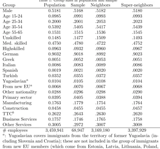
6.4. Firm size effects

Another issue closely related is a potential firm size effect: Is it possible that the effect of a high correlation of living together and working together is driven by individuals working in large establishments? Or are referrals especially in small firms more important, as information flows easier in small establishments and employers in small firms are most likely to rely on informal job markets?

To get an idea whether the network effect we measure is actually only spurious correlation generated by firm sizes or whether small firms are actually better

(23)

Table 5: Firm size effects for referrals to a neighborhood

Variable Small firms Small f. males Medium firms Large firms

Constant 1.8344^∗∗∗ 1.764^∗∗∗ 1.4818^∗∗∗ 2.0055^∗∗∗

(.0018) (.0025) (.0016) (.0074)

Rij .1300^∗∗∗ .1062^∗∗∗ .0756^∗∗∗ .1490^∗∗∗

(.0115) (.0160) (.0105) (.0477)

Relative increase [7.1%] [9.0%] [5.1%] [7.4%]

σu 3.3893 1.6823 3.4128 4.3674

σε 13.4182 10.7988 12.0897 13.9568

# pairs 74.2 Mio 18.1 Mio 47.3 Mio 59.8 Mio

# groups 10785 9343 10474 10535

Corr(u, Xb) -.0090 -.0052 -.0058 .0048

Heteroscedasticity-consistent standard errors in parentheses. [ ] gives increase in probability of working together^∗/^∗∗/^∗∗∗mark significance at the 90%/95%/99% confidence level.

Small firms: <50 employees, medium: 50-249 employees, large: ≥250 employees.

transmitter of information, we estimate our baseline specification for three different subsets. First we re-estimate equation 1 for pairs of individuals of whom the neighborsjare working in small or tiny firms (less than 50 employees). The second category are medium sized firms, where j work in establishments with 50 to less than 250 employees. Third we look at a subset of neighbors who work in large establishments, defined as those larger than 250 employees.

Again we differentiate between referrals to a neighborhood and to a firm. We are especially concerned of biased results in the small size category, because here we should have many family businesses, where people work and live together as a result of belonging to one household. As we cannot identify members of one household in our data set, we estimate the equation for small firms for males only. For both specificationsathe results do not differ significantly.

Table 5 shows the probability of working in the same neighborhood whenjworks in different sizes of establishments. We observe no systematic difference by firm size. Both absolute and relative increases in probability are fairly similar to our baseline specification, with medium firms having the smallest effect. Working in the same neighborhood with people from one’s super-neighborhood (constant) is most likely for large firms, a small hint towards a size effect. Regarding the relative effect, the magnitude is in line with our other specifications.

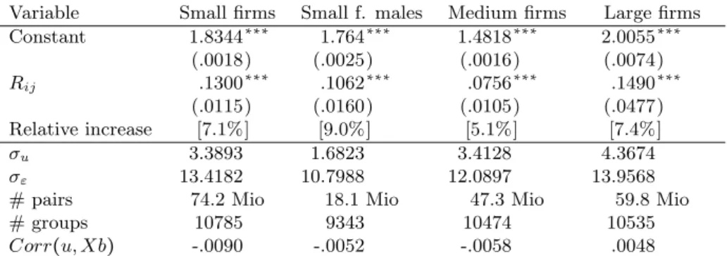
More interestingly we observe in table 6 huge increases in the relative probability of working in the same small firm, which are also highly significant.

Excluding females from the sample does not change this result, but leaves both absolute and relative effect unchanged. When j is working in a medium size establishment, the probability of working with a neighbor is comparable to that in the whole sample, whereas the relative effect is smallest and least precisely

(24)

Table 6: Firm size effects for referrals to a firm

Variable Small firms Small f. males Medium firms Large firms

Constant .0156^∗∗∗ .01711^∗∗∗ .0880^∗∗∗ .5788^∗∗∗

(.0001) (.0004) (.0013) (.0074)

Rij .0217^∗∗∗ .0233^∗∗∗ .0418^∗∗∗ .1275^∗∗∗

(.0011) (.0023) (.0081) (.0472)

Relative increase [139.9%] [136.3%] [47.6%] [22.02%]

σu 1.7040 .5687 1.0772 4.3674

σε 1.3745 1.4367 3.0664 13.9568

# pairs 74.2 Mio 18.1 Mio 47.3 Mio 59.8 Mio

# groups 10785 9343 10474 10535

Corr(u, Xb) .0036 .0061 .0162 .0048

Heteroscedasticity-consistent standard errors in parentheses. [ ] gives increase in probability of working together. ^∗/^∗∗/^∗∗∗mark significance at the 90%/95%/99% confidence level.

Small firms: <50 employees, medium: 50-249 employees, large: ≥250 employees.

estimated²⁷ in case of large firms. Although we do not want to stress causal interpretation here, as our subsets are selective, we see these results as a clear indication that our estimates are not driven by a pure size effect meaning people are only working with their neighbors because they all work in big firms. In contrast, small establishments seem to be best suitable for referring someone from your network, maybe because employers rely more heavily on informal referrals or because information flows easier in small plants. This result is also in line with Hellerstein et al. (2011).

6.5. Commuting

To get further insight into the nature of the measured referral effects, we explicitly address the effect of commuting behavior. We are concerned that our measured effect could be driven by a disproportionately high number of short distance commuters who locate close to their work place and hence have a high probability of working with their neighbors. Therefore, we exclude all individuals working in the same zip code area as they live in and reestimate equation 1 with this restricted sample to test whether the coefficient of social interaction α0 differs significantly from that in the full sample. Table 7 summarizes the results for referrals to a neighborhood and referrals to a firm. The sample size is restricted to 154.2 million pairsij, which means that excluding all individuals who live where they work does not reduce the data set fundamentally, but there seems to be only a minority of individuals working at their residential location.

Furthermore, both the constant and the social interaction effect remain at a

27Albeit being significant on a 1% level, the 95% confidence interval ofRijgoes from 0.0349 to 0.2201, which is large considering the sample size.