Modeling Multivariate Time Series with Fractional Integration in Macroeconomics and Finance

(1)

Modeling Multivariate Time Series with Fractional Integration in Macroeconomics

and Finance

Dissertation zur Erlangung des Grades eines Doktors der Wirtschaftswissenschaft

eingereicht an der

Fakultät für Wirtschaftswissenschaften der Universität Regensburg

vorgelegt von Roland Weigand

Berichterstatter:

Prof. Dr. Rolf Tschernig, Universität Regensburg Prof. Dr. Enzo Weber, Universität Regensburg

Tag der Disputation: 17. Juli 2014

(2)

List of Figures

4.1 ARMA(2,2) coefficients in the approximation of fractional processes for

−0.5<d<1 andn=500 . . . 62

4.2 Impulse responses for different approximations of fractional processes . . 63

4.3 Root mean squared approximation error for different approximations of fractional processes,−0.5<d<0 andn=500. . . 65

4.4 Root mean squared approximation error for different approximations of fractional processes, 0<d<1 andn=500 . . . 66

4.5 Time series plot of log realized variances . . . 67

4.6 Time series plot of z-transformed realized correlations . . . 68

4.7 Residual plot from the estimated DOFC model . . . 74

4.8 Residual autocorrelations from the estimated DOFC model . . . 75

4.9 Autocorrelations of squared residuals from the estimated DOFC model . . 76

4.10 Histogram of residuals from the estimated DOFC model . . . 77

4.11 Selected smoothed fractional and nonfractional components from the estimated DOFC model . . . 78

5.1 Time series plots and kernel densities for different transforms of realized covariance matrices . . . 95

5.2 Robustness of out-of-sample results with respect to the order specification of the VARMA model . . . 103

5.3 Robustness of out-of-sample results with respect to specification of dynamic persistence . . . 105

5.4 Robustness of out-of-sample results with respect to order specification of the CAW models . . . 106

(5)

List of Tables

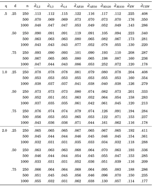
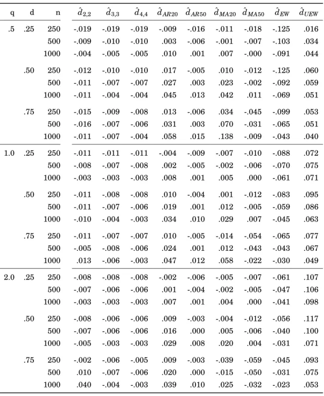
4.1 Root mean squared errors for data generating process of section 4.4.1 . . . 38 4.2 Bias for data generating process of section 4.4.1 . . . 40 4.3 Root mean squared errors for data generating process of section 4.4.2 . . . 42 4.4 Median errors for data generating process of section 4.4.2 . . . 44 4.5 Root mean squared errors for data generating process of section 4.4.3 with

r=0.5 . . . 45 4.6 Root mean squared errors for data generating process of section 4.4.3 with

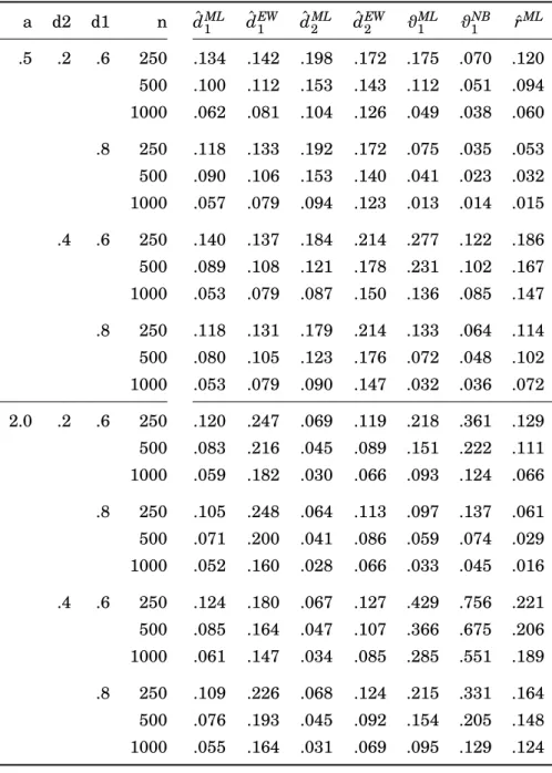
r=1 . . . 47 4.7 Root mean squared errors for data generating process of section 4.4.4 with

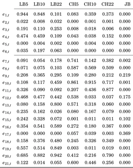
a=0.5 . . . 49 4.8 Estimation results for different specifications of the DOFC model . . . 56 4.9 P-values of diagnostic tests for the residuals from the estimated DOFC

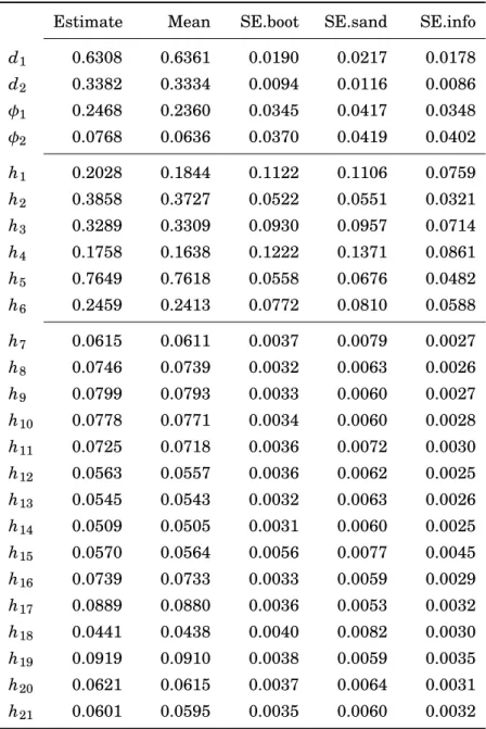
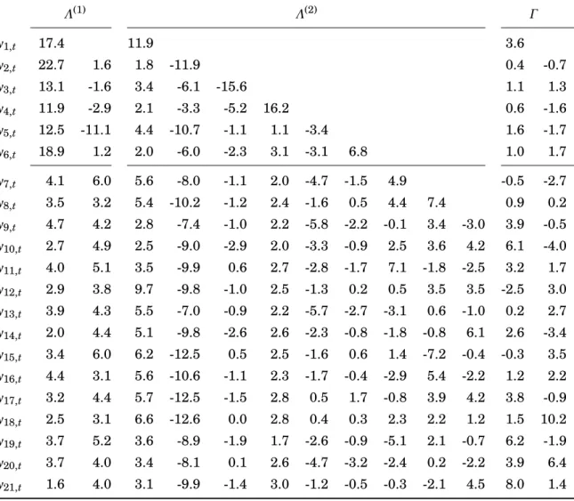
model . . . 57 4.10 Estimated parameters, bootstrap mean and standard errors from the DOFC

model . . . 58 4.11 Bootstrap t-ratios for fractional components loadings from the estimated

DOFC model . . . 59 4.12 Out-of-sample risks of DOFC model and several benchmarks,h=1 . . . . 62 4.13 Out-of-sample risks of DOFC model and several benchmarks,h=5 . . . . 63 4.14 Out-of-sample risks of DOFC model and several benchmarks,h=10 . . . . 64 4.15 Out-of-sample risks of DOFC model and several benchmarks,h=20 . . . . 64 5.1 Estimates of the transformation parameters in the MBC-RCov model . . . 92 5.2 Estimates of the transformation parameters for the realized variances in

the BC-DC model . . . 94 5.3 Number of rejections for univariate diagnostic residuals tests based on

different transformations . . . 97 5.4 Fraction of mean Frobenius loss between bias-corrected and naive forecasts.100

(6)

5.5 Out-of-sample Frobenius risks and logarithmic predictive density of MBC and BC-DC models and several benchmarks . . . 101 5.6 Out-of-sample Stein and L3 risks of MBC and BC-DC models and several

benchmarks . . . 108 5.7 Out-of-sample realized variance of minimum variance portfolio and squared

daily return of minimum variance portfolio of MBC and BC-DC models and several benchmarks . . . 109

(7)

1 Introduction and Overview

This thesis develops new approaches for modeling multivariate time series. It covers four essays on different setups from macroeconomics and finance. In the introduction, first the general framework of multivariate time series models is introduced with a mention of long-memory processes and factor models. Then, the empirical setups of the essays are outlined, while a third section states the contribution of this dissertation relative to the existing literature and gives an overview over the essays.

1.1 Methodological Framework

In this dissertation we consider collections of k economic variables y_t =(y1t, . . . ,y_kt)⁰ which are measured regularly at time periods t=1, . . . ,T. The aim is a model-based statistical characterization of the dependencies between elements of y_t over time and among each other, which may serve different purposes. In macroeconomics, multivariate time series models have been used for analysing the effects of structural shocks which we denote by a vector εt. Elements of this process are associated with inter- pretable economic sources of fluctuations whose dynamic impacts on the observable series in y_t are studied. Moreover, such models are applied for forecasting. Here, the dependence of the economic variables over time is used to draw conclusions on the prob- abilistic behaviour of y_T+h in the future, given currently available information y₁, . . . , y_T.

A very influential approach which has fostered numerous applications since its introduction to macroeconomics by Sims (1980) is the vector autoregressive (VAR) model

y_t=A₁y_t₋₁+. . .+A_py_t₋_p+u_t, t=1, . . . ,T; (1.1) see Lütkepohl (2005) for a textbook treatment. Here, u_t is an independent and iden- tically distributed disturbance term with zero mean and covariance matrixΣ, denoted u_t∼I I D(0,Σ), while correlation between observations over time is introduced by lagged values y_t₋_l, l=1, . . . ,p, which enter the model equation through the (k×k) coefficient

(8)

matricesA_l. NondiagonalA_l and contemporaneous correlation between the noise com- ponentsu_tallow for dynamic linkages between the individual time series under consideration.

A large literature has considered the long-run behaviour of systems such as (1.1). In general, unit roots in the characteristic equation|I−A₁z−. . .−A_pz^p| =0 induce nonstationary time series with stochastic trends, most prominently processes which are called integrated of order 1 orI(1), but alsoI(d) processes withd=2, 3, . . . are possible. These can be rendered stationary autoregressive moving average (ARMA) processes, classified as I(0), by d-th order differencing. Such difference-based modelling has been brought forward in applied statistics by Box and Jenkins (1970). The notion of long-run equilib- ria betweenI(1) processes, so-called cointegration relations, has propelled the emphasis on the long-term properties of economic time series in recent decades, beginning with Granger (1983), Granger and Weiss (1983) and Engle and Granger (1987).

The VAR model is very popular among applied researchers but has shortcomings in several fields of empirical work. A major limitation of the VAR setup is the dichotomy between stationary I(0) processes and the unit root case. This amounts to a sharp distinction between the rather extreme cases of short and perfect memory, respectively, and poses a considerable challenge to distinguish between these setups, especially when structural analyses and forecasts are sensitive with respect to the specification of the long-run properties. The unit root testing methodology often fails to provide a clear answer, and hence, different treatments of certain variables co-exist in the literature.

Additionally, processes of interest are often relatively high-dimensional which causes problems for VAR analysis. Given a k-dimensional time series y_t, the number of free parameters in the unrestricted VAR (1.1) is k²p+0.5k(k+1) and grows quadratically ink. Such a parameter affluence hinders precise estimation for largerk and limits the scope of VAR models to applications with a few variables only. Methodological progress has been spurred by these drawbacks of VARs for modeling the correlation structures, but also analyses from a new perspective have extended the scope of multivariate time series modeling; for example to time varying conditional covariance matrices; see Boller- slev, Engle, and Wooldridge (1988).

In this thesis, the mentioned shortcomings are tackled in different empirical setups, where the integration properties of the multivariate systems will be a primary focus.

With this respect, fractionally integrated time series models are considered which avoid

(9)

theI(0)/I(1) dichotomy by use of the fractional difference operator

∆^d=(1−L)^d= X∞ j=0

πj(d)L^j, π0(d)=1, πj(d)= j−1−d

j πj−1(d), j=1, 2, . . . , where L denotes the lag operator (L y_t = y_t−1) and d is a possibly non-integer scalar;

see Baillie (1996) for a review. As a straightforward multivariate approach one may consider modeling thefractionally differencedprocess as a stationary VAR,

(I−A₁L−. . .−A_pL^p) (∆^d¹^y1t, . . . ,∆^d^k^ykt)⁰=u_t, t=1, . . . ,T; (1.2) see Sowell (1989) for an early treatment of fractionally integrated vector ARMA models and Nielsen (2004) who considers the fractionally integrated VAR (1.2) as a special case.

The individual series y_itare integrated of fractional orders d_i which straightforwardly extends the classification intoI(d) variables for integerd. Analogously to the unit root literature, models with (fractional) cointegration have been developed and applied since the seminal work of Cheung and Lai (1993); see, e.g., Robinson and Hualde (2003) and Johansen and Nielsen (2012).

To cope with high dimensionality (large k) in time series analysis, which is also a key topic in this thesis, factor models have been a particularly successful field of research. Geweke (1977) extended classical cross-sectional factor analysis to a dynamic setup, while Quah and Sargent (1993) provided evidence on its applicability to the high- dimensional case. An elementary factor model is given by

y_t=Λf_t+εt, t=1, . . . ,T, (1.3) where f_t is anr-dimensional unobserved process which may be modelled as a VAR like (1.1), and where r<k. The assumptions onεt are crucial for a possible parsimonious parametrization for large k. The econometric literature has considered high-dimensional approximate factor models where, loosely speaking, f_t accounts for the bulk of cross-sectional correlation between elements of y_t (see Bai and Ng, 2008, for a survey).

In contrast, the terminus of a statistical factor model has been used for setups where εt is serially uncorrelated and therefore, f_t accounts for the autocorrelation and hence for dimension-reduced dynamics in y_t (Pan and Yao, 2008; Lam, Yao, and Bathia, 2011;

Lam and Yao, 2012).

(10)

1.2 Empirical Setups and Motivation

From an empirical point of view, this thesis is concerned with two distinct setups. The framework in chapters 2 and 3 is a bivariate time series with a focus on structural analysis, while the applications of chapters 4 and 5 aim on forecasting higher dimensional processes of realized covariance matrices.

In the first setup, structural shocksεt enter a system similar to (1.1) asu_t=Bεt, and identification of the elements ofB is achieved by imposing that a certain shock (ε2t in our notation) has no long-term effect on a specified variable (y_1t). This is the well-known long-run restriction of Blanchard and Quah (1989) in theI(1) case. Chapter 3 considers a system of output and prices. Here, the identification scheme is motivated by a possible association of restricted shocks (ε2t) with aggregate demand shocks and unrestricted shocks (ε1t) with shocks on the aggregate supply side of the economy. Other important empirical work has been done in similar frameworks. Most notably, applications to output and unemployment (Blanchard and Quah, 1989) as well as to productivity and hours worked (Gali, 1999) have aroused widespread interest.

In a large part of the related literature, the specification of long-run properties have been crucial for the outcomes. In the productivity and hours worked setup, a large de- bate has emerged over the effect of a technology shock (ε1t) on hours worked (y_2t). Mod- eling hours worked asI(1) and hence in first differences, a negative effect is found (Gali, 1999), while a specification in levels yields a contradictory conclusion with a positive effect; see Christiano, Eichenbaum, and Vigfusson (2003) and Christiano, Eichenbaum, and Vigfusson (2007). Similarly, for the output and price system considered in this thesis, Bayoumi and Eichengreen (1994) use an I(1) specification for prices (y_2t) and find a negative effect ofε1t (supply shocks) on prices, while in Quah and Vahey (1995), the effect of the non-core inflation shock (as they interpretε1t) on prices is positive but not significant for theirI(2) specification. Such ambiguities and their possible resolution by fractional integration techniques constitute the agenda for the first part of this thesis.

The second empirical setup of this thesis is concerned with modeling and forecasting the volatility of multiple financial assets. A relatively new literature has studied the dynamics of realized covariance matrices. Here, intra-day data on transaction prices are used to compute variances and covariances of asset returns within each trading day. Forecasts of the latter have been found valuable, e.g., for the purpose of portfolio selection (Liu, 2009).

From the perspective of dynamic modeling, standard approaches such as (1.1) exert the aforementioned problems. The strong persistence in the series has been tackled

(11)

by fractional integration techniques in the literature (Chiriac and Voev, 2011), while the typically high dimensionality of the series has led researchers to consider different forms of factor models; see Bauer and Vorkink (2011), Golosnoy and Herwartz (2012) and Gribisch (2013).

Another crucial distinction between the approaches considered in the literature is through the different transforms applied to the realized covariance matrices before fitting dynamic models. Chiriac and Voev (2011) use the elements of a triangular matrix square-root, while the matrix logarithm has been considered among others by Bauer and Vorkink (2011). Likewise, approaches that separate variance and correlation dynamics have been used; see Golosnoy and Herwartz (2012) and Halbleib and Voev (2011). In sum, the joint findings of long memory and factor structures poses a challenge to empirical researchers as does the coexistence of several transformations. The second part of this thesis is devoted to these problems.

1.3 Overview and Contribution

Despite the different setups, we employ similar strategies in the following chapters of this thesis. Implicitly or explicitly motivated by an empirical application, we identify key features of observed time series along with the problems which are most severe when standard methods are applied. In response, new modeling frameworks are developed which are well-suited to the empirical setups under consideration but also relevant in a wide range of other applications. For each of the models, econometric estimation poses further difficulties which are also tackled in this thesis.

The universe of existing approaches related to each of our empirical setups is char- acterized by certain dichotomies which turn out to be very influential for the outcomes of empirical work. Such discrete modeling choices may be harmful since they exclude possibly favorable in-between situations from the consideration set. Additionally, when deciding between the alternatives, there is typically no way to quantify an often substantial uncertainty regarding this decision in further steps of the analysis.

The methods we introduce are designed to overcome such dichotomies in the model specification process, most notably the distinction between integer integration orders.

The key concept with this respect is the use of fractional integration techniques and their suitable adaptation to the characteristics of our empirical setups. Transformations of the variables are another important instance of such modeling decisions. We avoid the latter using a continuous framework in the spirit of Box and Cox (1964) which we

(12)

propose for the dynamic modeling of realized covariance matrices. To be more explicit on the contribution of this thesis we consider each of the essays in turn.

Long- versus Medium-Run Identification in Fractionally Integrated VAR Mod- els. The following two chapters of this thesis extend structural VAR models with long- run restrictions to the case of fractional integration and hence overcome the dichotomy of integer orders which is typical for the related empirical literature. Chapter 2 is concerned with the interpretation of long-run restrictions to identify B when integration orders are non-integer. Whenever y_1t is integrated of an order less than one, these restrictions lose their original meaning from the I(1) setup. In this case, the structural shocks do not exert a non-vanishing influence on y_1t regardless of the identification constraints. This case is empirically very relevant, since key macroeconomic variables such as output have been found mean-reverting I(d) with d<1; see, e.g., Diebold and Rudebusch (1989).

To obtain an economically meaningful restriction for this case, we consider a medium- run approach that constrains the variance contributions ofε2t to y_1,t₊_hover finite horizons h. For different such identification schemes, we investigate the case where relatively long horizons are appropriate from economic theory. Formally, we show that let- ting the horizon tend to infinity is equivalent to imposing the restriction of Blanchard and Quah (1989) introduced for the unit-root case. This finding justifies the use of a computationally straightforward approach in practice, while it retains interpretability of the resulting shocks and thus helps to overcome the dichotomy of integer integration orders in a range of empirically relevant situations.

Long-run Identification in a Fractionally Integrated System. In this paper, a model is proposed which has increased flexibility for structural analysis as compared to existing fractional processes. We derive the model’s Granger representation and investigate the effects of long-run restrictions. In this way, we show that the impulse responses of y_1t to the restricted structural shockε2t are undesirably constraint for fractionally integrated VARs like (1.2), while our proposed FIVAR_b model allows for very general patterns of decay.

Both in simulations and in empirical work, we find that enforcing integer integration orders can have severe consequences for impulse responses and hence, that it is in- deed crucial to overcome this restrictive assumption in the current setup. Additionally, for the case of deterministic trends, a two-step estimation approach is proposed which outperforms the maximum likelihood estimator in a Monte Carlo study by Tschernig,

(13)

Weber, and Weigand (2013a).

In a system of U.S. real output and aggregate prices, shocks that are typically inter- preted as demand disturbances have a very brief influence on gross domestic product if prices are modeled as I(2) and exert a long-living effect if prices are taken to be I(1).

The fractional specification points to an in-between scenario, both in terms of the estimated integration orders and in the characterization of restricted impulse responses which are relatively short-living and hence closer to theI(2) specification.

State Space Modeling of Fractional Cointegration. Chapter 4 of this thesis also considers multivariate fractionally integrated time series models, albeit with a different scope. A model setup is proposed which allows for fractional cointegration relations between the variables and is thus more general than the models of the previous chapters. In contrast to the autoregressive nature of (1.2), the model is formulated in terms of latent fractional and additive short memory components. This approach allows for a treatment of possibly nonstationary time series of different fractional integration orders. It features cointegration relations of different strengths and is therefore very flexible as compared to currently applied parametric models such as Robinson and Hualde (2003), Johansen (2008) or Avarucci and Velasco (2009). A further advantage is the clear interpretation of the cointegration properties in our representation.

The empirical setup of realized covariance matrices motivates the use of parsimonious models which are applicable to processes consisting of a large number of variance and covariance processes or transformations thereof. With a factor structure as in (1.3), our unobserved components formulation benefits the modeling of such high-dimensional series. We propose an according parametrization of the fractional components setup which is based on dimension reduction along the lines of statistical factor models and dynamic orthogonal components (Matteson and Tsay, 2011).

Estimation of our model is based on a state space representation where finite order ARMA approximations of the fractional processes are applied. This procedure outperforms the standard autoregressive or moving average truncation approach by providing a substantial reduction in state dimension for a desired approximation quality and is hence computationally convenient. Monte Carlo simulations document the successful- ness of our approximation and show a reasonable performance of the proposed methods for cointegration modeling.

The methods are applied to realized covariance matrices using the dataset of Chiriac and Voev (2011). The sample consists of six U.S. stocks corresponding to a 21-dimensional time series of log variances and z-transformed correlations. It exhibits long memory

(14)

characteristics and a pronounced co-movement in the series’ low-frequency dynamics.

We find that common mutually orthogonal short- and long-memory components with two different fractional integration orders provide a reasonable fit to the data. An out-of-sample study shows that the fractional components model provides a superior forecasting accuracy compared to several competitor methods.

Matrix Box-Cox Models for Multivariate Realized Volatility. In the same framework of modeling realized covariance matrices, chapter 5 is concerned with data transforms and presents a flexible setup generalizing the Box-Cox approach (Box and Cox, 1964) to the matrix case. By proposing two specific models we face the otherwise discrete transformation decisions inherent to the modeling of realized covariance matrices.

The matrix Box-Cox model of realized covariances (MBC-RCov) is based on transformations of the covariance matrix eigenvalues, while for the Box-Cox dynamic correlation (BC-DC) specification the variances are transformed individually and modeled jointly with the z-transformed correlations.

A key part of this paper is concerned with parameter estimation. A multivariate semiparametric estimator is proposed for the transformation parameters and feasible confidence intervals are derived. The estimator allows for a convenient two-step modeling strategy, first determining the transform, while specifying a dynamic model in a second step.

Since an emphasis in this empirical framework is on forecasting, we also provide a discussion of bias-corrected point forecasts for re-transformed covariance matrices and of density forecasts for daily returns. A simulation-based approach is proposed which is applicable also for other models from the realized covariance literature and which we find very valuable in an out-of-sample evaluation.

Using the same dataset as in chapter 4, our estimates suggest negative Box-Cox transformation parameters close to zero for both the MBC-RCov and the BC-DC model.

The same values are supported by an out-of-sample forecast comparison. Here, the BC- DC model outperforms a wide range of competitor methods such as Cholesky-based and conditional Wishart models. In sum, modeling of log variances along with z-transformed correlations appears as a practically reasonable strategy, which also justifies the use of this transform in chapter 4.

Since this dissertation consists of four autonomous papers, the notation used in the following chapters differ and will be introduced for each chapter in turn. In the next two chapters, boldface symbols are used for vectors and matrices which reflects the practice in the published articles.

(15)

2 Long- versus Medium-run Identification in Fractionally Integrated VAR Models

This paper is joint work with Rolf Tschernig (University of Regensburg) and Enzo We- ber (University of Regensburg, Institute for Employment Research (IAB) and Institute for East and Southeast European Studies). It is published as T^SCHERNIG, R., E. W^E-

BER,^ANDR. W^EIGAND(2014): “Long- versus Medium-run Identification in Fractionally Integrated VAR Models,”Economics Letters, 122(2), 299–302.

(16)

3 Long-run Identification in a

Fractionally Integrated System

This paper is joint work with Rolf Tschernig (University of Regensburg) and Enzo We- ber (University of Regensburg, Institute for Employment Research (IAB) and Institute for East and Southeast European Studies). It is published as T^SCHERNIG, R., E. W^E-

BER, ^AND R. W^EIGAND (2013c): “Long-Run Identification in a Fractionally Integrated System,”Journal of Business & Economic Statistics, 31(4), 438–450.

(17)

4 State Space Modeling of Fractional Cointegration Subspaces

Abstract. We investigate a setup for fractionally cointegrated time series which is formulated in terms of latent integrated and short-memory components. It accommo- dates nonstationary processes with different fractional orders and cointegration of different strengths and is applicable in high-dimensional settings. A convenient parametric treatment is achieved by finite-order ARMA approximations in the state space representation. Monte Carlo simulations reveal good estimation properties for processes of different dimensions. In an application to realized covariance matrices, we find that orthogonal short- and long-memory components provide a reasonable fit and outstanding out-of-sample performance compared to several competitor methods.

Keywords. Long memory, fractional cointegration, state space, unobserved components, factor model, realized covariance matrix.

JEL-Classification. C32, C51, C53, C58.

4.1 Introduction

Multivariate fractional integration and cointegration models have proven valuable in a wide range of empirical applications from macroeconomics and finance. They generalize the standard concept of cointegration by allowing for non-integer orders of integration both for the observations and for equilibrium errors; see Gil-Alana and Hualde (2008) for a literature review. In the field of macroeconomics, such models have turned out to be relevant in analyses of purchasing power parity beginning with Cheung and Lai (1993), of the relation between unemployment and input prices (Caporale and Gil-Alana, 2002) and of broader models for economic fluctuations (Morana, 2006). The empirical finance literature has considered fractional cointegration, e.g., for analysing international bond

(18)

returns (Dueker and Startz, 1998), for modeling co-movements of stock return volatili- ties (Beltratti and Morana, 2006), for assessing the link between realized and implied volatility (Nielsen, 2007) and for quantifying risk in strategic asset allocation problems (Schotman, Tschernig, and Budek, 2008). From a methodological point of view, semiparametric techniques for inference on the cointegration rank, the cointegration space and memory parameters have been very popular among empirical researchers, although the development of optimal parametric inferential methods for models with triangular or fractional vector error correction representations has recently made considerable progress (see, e.g., Robinson and Hualde, 2003; Avarucci and Velasco, 2009;

Łasak, 2010; Johansen and Nielsen, 2012).

Despite their flexibility and their computationally simple treatment, semiparametric models are limited in scope since they aim to describe low-frequency properties only and are hence not appropriate for impulse response analysis and forecasting. While semiparametric techniques have been developed to cope with multivariate processes of different integration orders and multiple fractional cointegration relations of different strengths (Chen and Hurvich, 2006; Hualde and Robinson, 2010; Hualde, 2009), there seems to be a lack of parametric models of such generality. Furthermore, the usual error correction and triangular models with their typically abundant parametrization are not deemed appropriate for time series of dimension, say, larger than five.

In this paper, we investigate models for multivariate fractionally integrated and cointegrated time series which are formulated in terms of latent purely fractional and additive short-memory components. With a “type II” definition of fractional integration (Robinson, 2005), this approach allows for a flexible modeling of possibly nonstationary time series of different fractional integration orders. It permits cointegration relations of different strengths as well as polynomial cointegration (multicointegration in the terminology of Granger and Lee, 1989), i.e., cointegration between the levels of some time series and their (fractional) differences, and guarantees a clear representation of the long-run characteristics. The unobserved components formulation benefits the modeling of relatively high-dimensional time series. For this situation we propose a parsimonious parametrization based on dimension reduction and dynamic orthogonal components in the spirit of Pan and Yao (2008) and Matteson and Tsay (2011). We analyse the models in state space form which allows for missing values and a seam- less treatment of additive seasonal, noise, break and cycle components familiar from structural time series models (Harvey, 1991).

Several authors have proposed fractional integration modeling by state space methods. Classical treatments of univariate stationary long memory include Chan and

(19)

Palma (1998), who study autoregressive fractionally integrated moving average (ARFI- MA) processes and Grassi and de Magistris (2012), who consider ARFIMA models with noise, structural breaks and missing values. Bayesian simulation-based techniques have been proposed by Hsu and Breidt (2003) for noise-perturbed ARFIMA models and Brockwell (2007) for a so-called generalized long-memory model, where the conditional distribution of the process nonlinearly depends on a latent ARFIMA process.

Multivariate treatments of models based on latent fractional components have mostly been studied by semiparametric approaches. Ray and Tsay (2000) use semiparametric memory estimators and canonical correlations to infer the existence of common fractional components, Morana (2004) proposes a frequency domain principal component estimator, Morana (2007) estimate components of a single fractional integration order by univariate permanent-transitory (or persistent-transitory) decompositions followed by a principal component analysis of the permanent (or persistent) components and Lu- ciani and Veredas (2012) estimate their fractional factor model by fitting long-memory models to the principal components of a large panel of time series. In a setup closest to ours, Chen and Hurvich (2006) suggest a semiparametric frequency domain methodology to identify and estimate cointegration subspaces which annihilate fractional components of different memory.

Parametric, likelihood-based methods for such models have so far been computationally demanding. Hsu, Ray, and Breidt (1998) discuss a Bayesian sampling algorithm for a bivariate process sharing one stationary long-memory component. More recently, Mesters, Koopman, and Ooms (2011) consider maximum likelihood estimation of stationary generalized long-memory models with one or more latent ARFIMA components.

They propose an importance sampling scheme to obtain exact maximum likelihood estimators, but the methods become numerically challenging for more than two latent long-memory factors.

We consider a computationally straightforward classical treatment of our linear model in state space form. An approximation of potentially nonstationary fractional integration using finite-order ARMA structures is adapted. This procedure outperforms the standard truncation approach and provides a substantial reduction of the state dimension for a desired approximation quality, hence reducing the computational burden.

Parameter estimation by means of the EM algorithm and analytical expressions for the likelihood score make the approach feasible even in high dimensions. In Monte Carlo simulations we study the performance of the proposed methods and quantify the accuracy of our state space approximation. For fractionally integrated and cointegrated processes of different dimensions we find favorable finite-sample estimation properties

(20)

also in light of alternative techniques.

The methods are applied to modeling and forecasting daily realized covariance matrices, where the strengths of our approach become apparent. In this setup, typically high-dimensional processes with strong persistence and a pronounced co-movement in the low-frequency dynamics are considered. In time series of log variances and z- transformed correlations for six US stocks, we find that common orthogonal short- and long-memory components with two different fractional integration orders provide a reasonable fit. A pseudo out-of-sample study shows that the fractional components model provides a superior forecasting accuracy compared to several competitor methods.

The paper is organized as follows. Section 4.2 introduces the general setup and a specific parsimonious model, section 4.3 discusses its state space form and maximum likelihood estimation, while in section 4.4 the estimation properties are investigated by means of Monte Carlo experiments. The empirical application to realized covariance matrices and a pseudo out-of-sample assessment are contained in section 4.5 before section 4.6 concludes.

4.2 Fractional Components Models

In this section, we introduce a general modeling setup and clarify its integration and cointegration properties. Furthermore, its relation to existing setups for multivariate integrated time series is discussed. A specific model appropriate for relatively high- dimensional processes is considered which will be the workhorse specification in the empirical application of section 4.5.

4.2.1 The General Setup

We consider a linear model for a p-dimensional observed time series y_t, which we label afractional components(FC) setup,

y_t=Λx_t+u_t, t=1, . . . ,n. (4.1) The model is formulated in terms of the latent processesx_t and u_t whereΛwill always be assumed to have full column rank and the components of the s-dimensional x_t are fractionally integrated noise according to

∆^d^j^xjt=ξjt, j=1, . . . ,s. (4.2)

(21)

For a generic scalard, the fractional difference operator is defined by

∆^d=(1−L)^d= X∞ j=0

πj(d)L^j, π0(d)=1, πj(d)= j−1−d

j πj−1(d), j≥1, (4.3) where L denotes the lag or backshift operator, Lx_t =x_t−1. We adapt a nonstationary type II solution of these processes (Robinson, 2005) and hence treatd_j≥0.5 alongside the asymptotically stationary cased_j<0.5 in a continuous setup, while setting starting values to zero,x_jt=0 fort≤0. Nonzero initial values have been considered for observed fractional processes by Johansen and Nielsen (2012), but are not straightforwardly han- dled for our unobserved processes. The solution is based on the truncated operator∆^−d₊ ^j (Johansen, 2008) and given by

x_jt=∆⁻₊^d^jξjt=

t−1X

i=0

ψi(d)ξj,t−i, j=1, . . . ,s.

Without loss of generality let the components be arranged such thatd₁≥. . .≥d_s. We assumed_j>0 for all jin what follows, so thatx_tgoverns the long-term characteristics of the observations y_t. These are complemented by additive short-run dynamics which we describe by stationary vector ARMA specifications foru_t in the general case.

The process is given by

Φ(L)u_t=Θ(L)e_t, t=1, . . . ,n, (4.4) where Φ(L) and Θ(L) are a stable vector autoregressive polynomial and an invertible moving average polynomial, respectively. The disturbances ξt and e_t jointly follow a Gaussian white noise (NID) sequence such that

ξt∼NID(0,Σ_ξ), e_t∼NID(0,Σe) and E(ξte⁰_t)=Σ_ξe, (4.5) where at this stage, before turning to identified and empirically relevant model specifications below, we do not consider restrictions on the joint covariance matrix, but only requireΣ_ξ to have strictly positive entries on the main diagonal.

Some remarks regarding the general FC setup are in order. The model as given in (4.1) is not identified without further restrictions on the loading matrixΛ, on the vector ARMA coefficients and on the noise covariance matrix. While restrictions on Σξ and Λ may be based on results in dynamic factor analysis as will be seen below, choosing specific parametrizations for u_t will depend on characteristics of the data and on the purpose of the empirical analysis. Identified vector ARMA structures like the echelon

(22)

form (see Lütkepohl, 2005, chapter 12) can be used for a rich parametrization, while a multivariate structural time series approach as described in Harvey (1991) integrates nicely with the unobserved components framework considered in this paper. Below, we introduce a parsimonious model well-suited to relatively high dimensions which is conceptually based on dimension reduction and orthogonal components.

For a characterization of the integration and cointegration properties of our model, we adapt the definitions of these concepts from Hualde and Robinson (2010), which prove useful here. Hence, a generic scalar processρt is called integrated of orderδor I(δ) if it can be written asρt=Pl

i=1∆^−δ₊ ⁱνit, where δ=max_i=1,...,l{δi} and νt=(ν1t, . . . ,νl t)⁰ is a finite-dimensional covariance stationary process with spectral density matrix which is continuous and nonsingular at all frequencies. A vector process τt is called I(δ) if δis the maximum integration order of its components. We call the process τt cointegrated if there exists a vector βsuch that β⁰τt is I(γ) where δ−γ>0 will be referred to as the strength of the cointegration relation. The number of linearly independent cointegration relations with possibly differingγis called cointegration rank ofτt.

By these definitions, x_jt is clearly I(d_j) while both x_t and y_t are integrated of order d₁. We observe at least two different integration orders in the individual series of y_t whenever Λi1 =0 for some i and d₁ > d₂. More generally, y_it ∼I(d_j), if Λi1 =. . .= Λi,j−1=0 butΛi j6=0.

To state the cointegration properties of the FC setup (4.1), we assume that s≤p, so that all fractional components are reflected by the integration and cointegration structure of y_t and that Σξ is nonsingular. It is useful to identify all q groups of x_jt with identical integration orders and denote their respective sizes by s₁, . . . , s_q, such that d_s₁₊_...₊_s_j

−1+1=. . .=d_s₁₊_...₊_s_j ands=Pq

j=1s_j. Of course, ifq=s, thens₁=. . .=s_q=1 and all components ofx_t have mutually different integration orders, while for q=1 it holds thats=s₁ and we observed₁=. . .=d_s.

To keep notation simple, for a generic matrix Afor which a specific grouping of rows and columns is clear from the context, we denote byA^(i,^j)the block from intersecting the i-th group of rows with the j-th group of columns. A stacking of several groups of rows i, . . . ,jand columnsk, . . . ,lis indicated byA^(i:^j,k:l). For a grouping in only one dimension we write A⁽ⁱ⁾ or A^(i:^j), where it shall be clear from the context whether a grouping of rows or columns is considered. Furthermore, we denote the column space of a generic k×l matrix A by s p(A)⊆R^k and its orthogonal complement by s p^⊥(A). Further, for k>l, thek×(k−l) orthogonal complement of Awill be denoted byA_⊥, which spans the (k−l)-dimensional spaces p^⊥(A).

According to the grouping of equal individual integration orders in x_t, we may there-

(23)

fore rewrite the FC process (4.1) as

y_t=Λ⁽¹⁾x⁽¹⁾_t +. . .+Λ^(q)x^(q)_t +u_t.

Here,Λ⁽^j)is a p×s_jsubmatrix ofΛconsisting of columnsΛ·ifor whichs₁+. . .+s_j−1<i≤ s₁+. . .+s_j, and x⁽_t^j) is a s_j-dimensional subprocess of x_t corresponding to components with memory parameter d⁽^j):=d_s₁_+...+s_j−1₊₁ =. . .=d_s₁_+...+s_j. Whenever s₁< p, there exist p−s₁ linearly independent linear combinations β⁰_iy_t ∼I(γi) andγi<d₁, so that fractional cointegration occurs. Due to our definition of cointegration, this may be a trivial case where a single component y_it with integration order smaller than d₁ is selected. Since

Λ⁽¹⁾_⊥⁰y_t=Λ⁽¹⁾_⊥ ⁰Λ⁽²⁾x⁽²⁾_t +. . .+Λ⁽¹⁾_⊥ ⁰Λ^(q)x^(q)_t +Λ⁽¹⁾_⊥⁰u_t

is integrated of order d⁽²⁾, the columns of Λ⁽¹⁾_⊥ qualify as cointegration vectors and S⁽¹⁾:=s p^⊥(Λ⁽¹⁾) is the (p−s₁)-dimensional cointegration space of y_t.

Whenever s₁+s₂ < p, there are subspaces of S⁽¹⁾ forcing a stronger reduction in integration orders. More generally, it holds thatΛ^(1:_⊥ ^j)⁰y_t∼I(d⁽^j+1)) wheneverPj

i=1s_i<p and where we set d⁽^j⁺¹⁾=0 for j>s. Analogously to Hualde and Robinson (2010), for s= p and j=1, . . . ,q−1, we call S⁽^j):=s p^⊥(Λ^(1:j)) the j-th cointegration subspace of y_t, for whichS^(q⁻¹⁾⊂. . .⊂S⁽¹⁾. For p>s, S^(q)⊂S^(q⁻¹⁾ is a further such subspace.

Cointegration vectors in S^(q) cancel all fractional components and hence reduce the integration order fromd₁to zero, the strongest reduction possible in our setup.

Besides this general pattern of cointegration relations, our model features an interesting special case with so-called polynomial cointegration, that is, cointegration relations where lagged observations nontrivially enter a cointegration relation. To see this possi- bility, consider a bivariate example similar to Granger and Lee (1989), whereq=p=2 andξ1t=ξ2t, so thatΣξ is singular andx_2t=∆^d¹⁻^d²^x1t. Augmenting the variables by a fractional difference as ˜y_t:=(y_1t,y_2t,∆^d¹⁻^d²^y2t)⁰, we obtain a three-dimensional system where levels ofy_tenter a nontrivial cointegration relation with a fractional difference to achieve a reduction in integration order fromd₁ to max{2d2−d₁, 0}<d₂; see equation (4.26) below for the cointegration space. Hence, our setup complements the model of Johansen (2008, section 4), which was the first to handle polynomial cointegration in a fractional setup.

(24)

4.2.2 Relations to Other Cointegration Models

In this section, we clarify the relation of the fractional components model (4.1) to popular existing representations for cointegrated processes and show how our model can be represented in alternative ways brought forward in the literature. While our model is among the most general setups with respect to its integration and cointegration properties, the additive modeling of short-run dynamics is new to the literature and gives rise to distinct parametrizations not possible within other representations in a similarly convenient way.

Error correction models. The most popular representation of cointegrated systems in theI(1) setting is the vector error correction form. Since an early mention by Granger (1986), in the fractionally integrated case, e.g., Avarucci and Velasco (2009), Łasak (2010) and Johansen and Nielsen (2012) have recently considered such models. In terms of the integration and cointegration properties, the fractional error correction setups are typically restricted to the special case with q=2 and s=p, such that the observed variables are integrated of orderd⁽¹⁾ and there exist p−s₁cointegration relations with errors of orderd⁽²⁾.

Defining the fractional lag operatorL_b:=1−∆^b (Johansen, 2008), we are able to derive the error correction representation for this special case of our model; see appendix 4.A. It is given by

∆^d⁽¹⁾^yt=αβ⁰L_d(1)−d⁽²⁾∆^d⁽²⁾^yt+κt, (4.6) where we findαβ⁰= −Λ⁽²⁾(Λ⁽¹⁾_⊥⁰Λ⁽²⁾)⁻¹Λ⁽¹⁾_⊥⁰ to precede the error correction term, while

κt:=M(Λ⁽¹⁾ξ⁽¹⁾_t +∆^d⁽¹⁾^ut)−αβ⁰(Λ⁽²⁾ξ⁽²⁾_t +∆^d⁽²⁾^ut) is integrated of order zero andMis defined in (4.29).

The model differs both from the models of Avarucci and Velasco (2009) and from the representation of Johansen (2008) in the way short-run dynamics are modeled. While the literature has considered (fractional) lags of differenced variables and possibly of error correction terms in the VECM representation, our setup generates autocorrelated κt through the introduction of a latentu_t. In practice, approximating our model by an autoregressive structure in∆^d⁽¹⁾^yt may lead to an abundance of parameters whenever u_t is reasonably parametrized and vice versa.

As we have discussed above, Johansen (2008) proposes a polynomially cointegrated generalization of his model which allows terms integrated of ordersd,d−bandd−2bin

(25)

the Granger representation (Johansen, 2008, theorem 9). Even compared to that specification, our model allows for more general patterns of integration orders and cointegration strengths. More in line with the generality envisaged in this paper, Tschernig, Weber, and Weigand (2013c, appendix A) present a model with error correction term and different integration orders, while Łasak and Velasco (2014) sequentially fit error correction models to test for cointegration relations of possibly different strengths.

Vector ARFIMA. An interesting special case of (4.1) occurs fors=pandΛ=I, where each series in y_itis driven by a single fractional component and y_it∼I(d_i). This resem- bles standard vector ARFIMA models with possibly different integration orders; see, e.g., Lobato (1997) who labels the more popular vector ARFIMA class considered here as “model A”. A frequently used submodel is the fractionally integrated vector autoregressive model discussed by Nielsen (2004). The main difference to these approaches is our additive modeling of short-run dynamics, whereas in the vector ARFIMA setup weakly dependent vector ARMA instead of noise processes are passed through the fractional integration filters.

Our model belongs to the class of vector ARFIMA processes for integer d_j∈{1,2,. . .}, but not for general fractional integration orders. For the case of integer d_j, note that (x⁰_t,u⁰_t)⁰ is a finite-order vector ARMA process, and hence y_t as a linear combination is itself in the ARMA class; see Lütkepohl (1984). For general vector ARFIMA processes, a similar conclusion does not hold. It is sufficient to consider a stylized univariate case of our model with p=s=1, where ∆^d^xt=ξt and (1−φL)u_t =e_t. First note that (∆^d^xt,ut)⁰has a vector ARMA structure, and hence (xt,u_t)⁰is a vector ARFIMA process.

Expanding (1−φL)∆^d^xt =(1−φL)ξt and (1−φL)∆^d^ut=∆^d^et, we can write the sum, belonging to the fractional components model class, as

(1−φL)∆^d^yt=(1−φL)ξt+∆^d^et. (4.7) The right hand side of this expression is not a finite-order MA process in general, as it has nonzero autocorrelations for all lags, and hence, the process does not belong to the ARFIMA class.

Triangular representations. The models discussed so far have restricted integration or cointegration properties as compared to our model. In contrast, Hualde (2009) and Hualde and Robinson (2010) have proposed a very flexible model which adapts the triangular form of Phillips (1991) and its generalization to processes with multiple unit

(26)

roots (Stock and Watson, 1993) to the fractional cointegration setup.

To derive the triangular representation for our model, we assume that the variables in y_t are ordered in a way thatΛ^(1:^j,1:^j)is nonsingular for j=1, . . . ,qand restrict attention to the case s= p. The variables are partitioned according to the groups of different integration orders inx_t as y⁽_t^j):=(y_s₁₊_...₊_s_j₋₁₊₁, . . . ,y_s₁₊_...₊_s_j)⁰, j=1, . . . ,q. The first block in the triangular system is

∆^d¹^y⁽¹⁾_t =Λ^(1,1)ξ⁽¹⁾_t +Λ^(1,2)∆^d¹⁻^d²ξ⁽²⁾_t +. . .+Λ^(1,q)∆^d¹⁻^d^qξ^(q)_t +∆^d¹^ut (:=ω⁽¹⁾_t ), (4.8) whereω⁽¹⁾_t is integrated of order zero. The general expression for the j-th block of the triangular system is derived in appendix 4.A for j=2, . . . ,q, and given by

∆^d⁽^j)^y_t⁽^j)=Λ⁽^j,1:(^j⁻¹⁾⁾(Λ^(1:(j⁻^1),1:(^j⁻¹⁾⁾)⁻¹∆^d^(j)^y_t^(1:(j−1))+ω^(j)_t (4.9)

= −B⁽^j,1)∆^d^(j)^y⁽¹⁾_t −. . .−B⁽^j,^j−1)∆^d⁽^j)^y⁽_t^j⁻¹⁾+ω⁽_t^j),

where also ω⁽_t^j) is integrated of order zero for j=2, . . . ,q. By inverting the fractional difference operators we obtain

B y_t=(∆⁻₊^d¹ω⁽¹⁾_t ⁰, . . . ,∆⁻₊^d^qω^(q)_t ⁰)⁰, (4.10) where B has a block triangular structure such that B^(i,i)= I and B^(i,^j) =0 for i< j.

A re-ordering of the variables in y_t yields the representation of Hualde and Robinson (2010).

This representation allows for a semiparametric cointegration analysis of our model using the methods of Hualde (2009) and Hualde and Robinson (2010). However, our model differs significantly from straightforward parametrizations of the triangular system, e.g., from assuming a vector ARMA process forωt, since in our setupωt as stated in (4.32) generally contains fractional differences that cannot be represented within the ARMA framework.

State space approaches. Bauer and Wagner (2012) have presented a state space canonical form for multiple frequency unit root processes of different (integer-valued) integration orders. Their discussion is based on unit root vector ARMA models which are separated in pure unit root structures and short-term dynamics. Although the anal- ogy to our model is striking, there are notable differences between their unit root and our fractional setup. Firstly, as discussed in the paragraph on vector ARFIMA mod-

(27)

els (see (4.7)), the fractional components setup (4.1) is not nested within a general class comparable to the vector ARMA models, which form the basis of the discussion in Bauer and Wagner (2012). Secondly, in their setting, the introduction of different integration orders is achieved by repeated summation of lower order integrated processes which themselves enter the observations to achieve polynomial cointegration. This is in contrast to the continuous treatment of integration orders in our (type II) fractional setup.

However, fractional components models could be constructed to straightforwardly extend the setup of Bauer and Wagner (2012). Using the fractional lag operatorL_b=1−∆^b instead of L in the short-run dynamic specification (4.4), a stable vector ARMA_b process can be defined by ˜Φ(L_b) ˜u_t=Θ˜(L_b)e_t under suitable stability conditions (Johansen, 2008, corollary 6). Then, replacingu_t by ˜u_t in the model setup (4.1) withd_j restricted to some multiple of b (dj =i_jb, i_j∈{1, 2, . . .}), the process y_t is in the class of vector ARMA_bmodels itself, while unit roots in the vector autoregressive polynomial generate the fractionalI(d_j) processes. Such a framework could be treated analogously to Bauer and Wagner (2012), but the restriction that all integration orders are multiples of b makes such a framework somewhat less flexible than ours.

4.2.3 A Dimension-reduced Orthogonal Components Specification

So far, we have considered a general modeling setup and discussed its integration and cointegration properties as well as its relation to existing approaches in the literature. We now turn to the discussion of a specific model from this class which bears potential for parsimonious modeling of long- and short-run dynamics in relatively high- dimensional applications. Besides its general interest, this will be the workhorse specification for the empirical application to realized covariance modeling in section 4.5.

To introduce the model and emphasize its restrictions as compared to (4.1), we de- compose the short-term dependent process u_t into an autocorrelated component, Γz_t, wherez_t is a vector ofs₀mutually uncorrelated components withs+s₀≤p, and a white noise componentεt, respectively. We label the result thedynamic orthogonal fractional components(DOFC) model,

y_t=Λ⁽¹⁾x⁽¹⁾_t +. . .+Λ^(q)x^(q)_t +Γz_t+εt, (4.11) wherex_t is generated by a purely fractional process (4.2) as above, while