(890) meson production at √ s = 7 TeV

ATLAS-CONF-2010-032 13/07/2010

ATLAS NOTE

ATLAS-CONF-2010-032

June 9, 2010

Observation of Ξ , Ω baryons and K

(890) meson production at √ s = 7 TeV

The ATLAS Collaboration

Abstract

We present an observation ofΞ, Ωbaryon andK^∗(890) meson production in proton- proton collisions at√s=7 TeV energy using data collected by the ATLAS experiment. The resonances have been reconstructed using a cascade decay vertex fitter. Clear signals of all three resonances are obtained in data.

1 Introduction

This note presents preliminary results on observation and production rate measurement ofΞ,Ωhyperons and K^∗(890) meson using cascade decay reconstruction. TheΞ, Ωresonances have decay channels with long-lived particles -K_S⁰ andΛ⁰in final state which also decay inside the ATLAS detector tracking volume. The hyperons are observed in the decay modes Ξ→πΛ(→ pπ) andΩ→KΛ(→ pπ). Both hyperon charged states are used in analysis. Due to their significant lifetimes both Ξ and Ω decay far from primary event vertex producing secondary vertices. The Λ decays produce tertiary vertices.

The secondary and tertiary vertices from such cascade decays can be reconstructed together by using a cascade vertex fitting approach. For the observation ofK^∗(890) meson the decay mode withK_S⁰ is used K^∗(890)→πK_S⁰(→ππ). TheK^∗(890) decays strongly, so in this case the secondary vertex coincides in space with the primary event vertex. Nevertheless the cascade description is still valid and in this note the K^∗(890) decay vertex is not required to coincide with the primary event vertex. The distance between the reconstructed secondary K^∗ vertex and the primary one was used as a tool to remove background because in general this distance is greater for fake cascades than for true ones.

The cascade candidates have been reconstructed with a specialized cascade reconstruction algorithm available in the ATLAS collaboration. This algorithm is able to fit any linked set of vertices (cascade) constraining the intermediate particles to point to their production vertices in cascade structure. It takes into account the exact ATLAS detector magnetic field and the material distribution inside the ATLAS Inner Detector [1].

TheK^∗(890) decay reconstruction results were compared with the detailed ATLAS Monte Carlo pre- dictions for non-diffractive minimum bias events generated with PYTHIA [3], using the default ATLAS MC09 tuning [4].

2 Reconstruction

The data collected by the ATLAS experiment [1] in 2010 at √s=7 TeV collisions with a minimum- bias trigger were used in this study. These data correspond to an integrated luminosity of approximately 250µb⁻¹, and were selected for stable beam conditions and a fully functional Inner Detector require- ments. Approximately 10⁷fully simulated Monte Carlo minimum bias events were used for comparison.

Only events with good reconstructed primary event vertex made of at least 3 tracks were kept for fur- ther analysis. After this selection the data statistics consisted of 1.30·10⁷ events and the Monte Carlo statistics consisted of 1.04·10⁷events.

In order to decrease combinatorics, the cascade decay reconstruction started by selecting goodΛ⁰ andK_S⁰ candidates. Only tracks withχ²<4 and at least 2 silicon (Pixel or SCT) hits were used in theV⁰ reconstruction. The requirement of only 2 silicon hits out of 11 possible on average in ATLAS tracker leaves enough space forV⁰decays and guarantees track reconstruction accuracy [2]. Additional selection criteria were different for theK_S⁰ andΛ⁰due to the different lifetimes and relevant backgrounds. For the K_S⁰ reconstruction the two participating tracks must be oppositely charged, have 2d impact parameters

|d0|with respect to primary event vertex greater than 1 mm and transverse momenta pT>150 MeV. For theΛ⁰reconstruction the more energetic track of oppositely charged track pair must havepT>500 MeV and an impact parameter |d₀|>0.3 mm, while the less energetic track must have p_T>150 MeV and

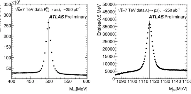
|d0|>0.5 mm. For each good track pair a vertex was reconstructed. TheK_S⁰ candidate vertex must have χ²<4 and the transverse flight distance greater than 5 mm. TheΛ⁰candidate vertex must haveχ²<5 and the transverse flight distance bigger than 10 mm. The invariant masses of K_S⁰ and Λ⁰ candidates which passed those criteria are shown in Fig. 1.

For the subsequent cascade decay search only theV⁰candidates within|M_ππ−M_K^PDG0s |<25 MeV and

|Mpπ−M_Λ^PDG0 |<8 MeV invariant mass windows were accepted. In this analysis the cascade consists

of 2 vertices. A primary cascade vertex corresponds to the Ξ, Ω, K^∗(890) decay and the secondary cascade vertex corresponds to theV⁰decay. Tracks from the preselectedV⁰candidates are provided to the cascade decay fitter to define the secondary cascade vertex. To define the primary cascade vertex an additional charged track together with the V⁰ trajectory from secondary cascade vertex are used.

The cascade vertex fitter assumes that the intermediate particle trajectory from the secondary cascade vertex passes exactly through primary cascade vertex constraining V⁰ momentum. Several additional constraints are allowed in the cascade fit, out of them only theV⁰ mass constraint is used in the current analysis. The cascade fitter recalculates the primary and secondary cascade vertex positions and momenta of participating tracks taking into account all the above constraints. In the current analysis the number of degrees of freedom of the cascade fit for all three resonances is three.

The selection of additional track (πforΞand K forΩ) and the cuts on fitted cascade parameters are tuned separately for the different resonances. They are presented below.

2.1 Ξreconstruction

The additional track for the primary cascade vertex must have at least 2 silicon (Pixel + SCT) hits, pT>150 MeV and|d0|>0.5 mm with respect to the primary event vertex. The pion mass hypothesis was used for this track in the fit. The reconstructed cascade candidate was accepted if it hadχ²<7 and the transverse distance between the primary event vertex and the primary cascade vertex was greater than 4 mm.

Different charge combinations of the 3 tracks in the cascade are possible. TheΞhyperon can de- cay into the pπ⁻π⁻+cc final state and cannot decay into pπ⁻π⁺+cc. The cascade candidates with the

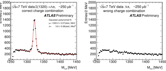
“wrong” charge combination can be used as a model-independent estimation of background under theΞ invariant mass peak. The results of theΞ→Λπcascade decay mode reconstruction for data are shown in Fig. 2. The invariant mass distributions for the correct and wrong track charge combinations are overlaid.

The separate distributions are presented in Fig. 5 for reference.

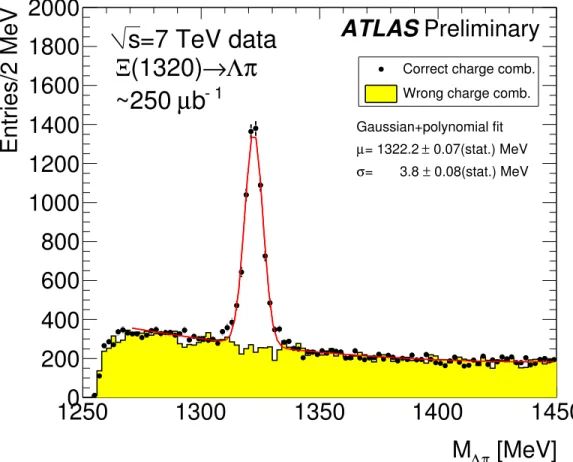
TheΞbaryon decay width is very small [5], so the reconstructed signal peak shape is determined by the detector resolution only. It is assumed to be a Gaussian. Then the Ξresonance invariant mass peak was fitted with the Gaussian plus polynomial distribution to find the mass and resolution. These fit results are shown in Fig. 2.

2.2 Ωreconstruction

The additional track for the primary cascade vertex must have at least 2 silicon (Pixel + SCT) hits, pT>400 MeV and|d0|>1 mm with respect to primary event vertex. The kaon mass hypothesis was used for this track in the fit. The reconstructed cascade candidate was accepted if it hadχ²<7 , the transverse distance between the primary event vertex and the primary cascade vertex was greater than 6 mm and the cascade pT (the transverse summary momentum of the three particles in the cascade recalculated by the fitter at the primary cascade vertex position) was greater than 1500 MeV. To exclude the kinematical reflection of the much more probableΞdecay with the same topology, the cascade mass was recalculated with the pion mass hypothesis for the third track and the cascade was rejected if this mass was in the

|M_Ξ^PDG−M_Λπ|<8 MeV invariant mass window. Similar to theΞdecay final state charges the Ωcan decay into the pπ⁻K⁻+cc final state and cannot decay into pπ⁻K⁺+cc. The cascade candidates with

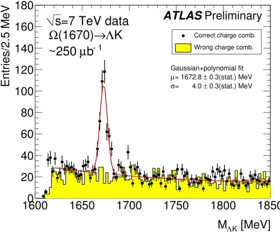
”wrong” charge combination were used as the model-independent estimation of background under theΩ invariant mass peak. The results of theΩ→ΛKcascade decay reconstruction are shown in Fig. 3 with the overlaid invariant mass distributions for correct and wrong track charges combinations. The separate distributions are presented in Fig. 6 for reference.

TheΩbaryon decay width is similar to theΞone and the invariant mass peak width is also deter- mined by the detector resolution. The standard Gaussian plus polynomial fit was used to extract signal

parameters. TheΩsignal peak in data is prominent, the mass is consistent with the PDG [5] value and the width is similar to theΞvalue for similar decay kinematics.

2.3 K^∗(890) reconstruction

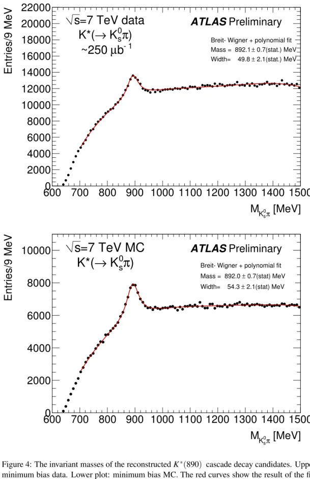
The K^∗(890) decays strongly and does not have a measurable decay length, so the selection of the additional track for the primary cascade vertex was different from the previous cases. The additional track for the cascade decay fit must now have at least 2 Pixel hits, one of them being a B-layer hit, pT>500 MeV and|d0|<0.25 mm with respect to the primary event vertex. The pion mass hypothesis was used for this track in the cascade fit. The reconstructed cascade candidate was accepted if it had χ²<7 , the transverse distance between the primary event vertex and the primary cascade vertex was smaller than 0.8 mm and the cascade p_T>1500 MeV. To reduce the background further the additional kinematical cut p^K_T^∗−p^π_T>1000 MeV was used. The reconstruction results are presented in Fig. 4 for data and Monte Carlo. No correct and wrong charge combinations can be identified here because theK_S⁰ decay is symmetric.

Contrary to theΞandΩresonances, theK^∗(890) has the decay width≈50 MeV [5] what is much bigger than the detector resolution. The invariant mass signal peak shape can’t be described by the Gaussian in this case. The nonrelativistic Breit-Wigner function plus polynomial fit was used to extract the K^∗(890) signal parameters. The masses and widths of signal peaks in data and Monte Carlo are consistent with each other and the PDG [5] values.

3 Results

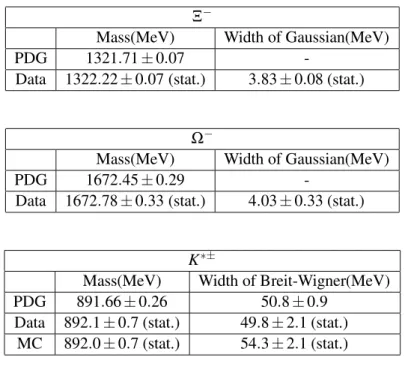
The results obtained after the cascade decay candidate reconstruction and signal fitting procedure are summarized in Table 1.

Ξ⁻

Mass(MeV) Width of Gaussian(MeV)

PDG 1321.71±0.07 -

Data 1322.22±0.07 (stat.) 3.83±0.08 (stat.)

Ω⁻

Mass(MeV) Width of Gaussian(MeV)

PDG 1672.45±0.29 -

Data 1672.78±0.33 (stat.) 4.03±0.33 (stat.)

K^∗±

Mass(MeV) Width of Breit-Wigner(MeV)

PDG 891.66±0.26 50.8±0.9

Data 892.1±0.7 (stat.) 49.8±2.1 (stat.) MC 892.0±0.7 (stat.) 54.3±2.1 (stat.)

Table 1: The cascade decay reconstruction results

4 Summary

The cascade decays Ξ→Λπ, Ω→ΛK and K^∗(890)→K_S⁰π have been successfully reconstructed in data recorded by ATLAS experiment in √s=7 TeV pp collisions using a cascade vertex fitter algo- rithm. When compared to the known masses of these particles [5], the fitted masses of the observed invariant mass peaks imply a momentum scale correct to better than 1%. These results demonstrate good performance of the ATLAS track and vertex reconstruction algorithms.

References

[1] The ATLAS Collaboration: The ATLAS Experiment at the CERN Large Hadron Collider, 2008 JINST 3 S08003

[2] The ATLAS Collaboration: Expected Performance of the ATLAS Experiment: Detector, Trigger and Physics, Chapter 2, “Tracking”, pp. 15, CERN-OPEN-2008-020 [arXiv:0901.0512]

[3] T. Sjostrand, S. Mrenna, and P. Skands, PYTHIA 6.4 Physics and Manual, JHEP 05 (2006) 026, arXiv:hep-ph/0603175.

[4] The ATLAS Collaboration: ATLAS Monte Carlo Tunes for MC09, ATL-PHYS-PUB-2010-002 [5] C.Amsler et al.(Particle Data Group), Review of Particle Physics, Physics Letters B667, 1 (2008)

[MeV]

π

Mπ

400 450 500 550 600

Entries/3 MeV

50 100 150 200 250 300 350×10³

b-1

), ~250 µ π

π (→

s0

=7 TeV data K s

Preliminary ATLAS

[MeV]

π

Mp

1090 1100 1110 1120 1130 1140 1150

Entries/0.5 MeV

0 5000 10000 15000 20000 25000 30000 35000 40000 45000 50000

b-1

µ ), ~250 π

p

→ ( Λ

=7 TeV data s

Preliminary ATLAS

Figure 1: The invariant masses of the preselected K_S⁰ and Λ⁰ candidates used for cascade decay re- construction. The vertical lines represent corresponding PDG masses - 497.61 MeV for K_S⁰ and 1115.68 MeV forΛ⁰.

[MeV]

π

M

1250 1300 1350 1400 1450

Entries/2 MeV

0 200 400 600 800 1000 1200 1400 1600 1800

2000 s =7 TeV data π Λ (1320) → Ξ µ b

~250

Preliminary ATLAS

Gaussian+polynomial fit 0.07(stat.) MeV

±

= 1322.2 µ

0.08(stat.) MeV

= 3.8 ± σ

Correct charge comb.

Wrong charge comb.

Figure 2: The invariant masses of the reconstructed Ξcascade decay candidates. The distributions for correct charge combinations and wrong charge combinations are overlaid. The red curve shows the result of the fit described in the text.

[MeV]

K

M

1600 1650 1700 1750 1800 1850

Entries/2.5 MeV

0 20 40 60 80 100 120 140 160

180 s =7 TeV data Λ K (1670) → Ω µ b

~250

Preliminary ATLAS

Gaussian+polynomial fit 0.3(stat.) MeV

= 1672.8 ±

µ= 4.0 ± 0.3(stat.) MeV σ

Correct charge comb.

Wrong charge comb.

Figure 3: The invariant masses of the reconstructed Ωcascade decay candidates. The distributions for correct charge combinations and wrong charge combinations are overlaid. The red curve shows the result of the fit described in the text.

[MeV]

sπ K0

M

600 700 800 900 1000 1100 1200 1300 1400 1500

Entries/9 MeV

0 2000 4000 6000 8000 10000 12000 14000 16000 18000 20000 22000

=7 TeV data s K*( → K

π )

b

~250 µ

2.1(stat.) MeV Width= 49.8 ±

Preliminary ATLAS

[MeV]

sπ K0

M

600 700 800 900 1000 1100 1200 1300 1400 1500

Entries/9 MeV

0 2000 4000 6000 8000 10000

Breit-Wigner + polynomial fit 0.7(stat) MeV Mass = 892.0 ±

2.1(stat) MeV Width= 54.3 ±

=7 TeV MC

s K*( → K

π ) ATLAS Preliminary

Figure 4: The invariant masses of the reconstructed K^∗(890) cascade decay candidates. Upper plot: real minimum bias data. Lower plot: minimum bias MC. The red curves show the result of the fit described in the text.

[MeV]

π

MΛ

1250 1300 1350 1400 1450

Entries/2 MeV

0 200 400 600 800 1000 1200 1400 1600 1800

2000 s=7 TeV data Ξ(1320)→Λπ, ~250 µb-1

correct charge combination

Gaussian+polynomial fit 0.07(stat.) MeV

±

= 1322.2 µ

0.08(stat.) MeV

±

= 3.8 σ

Preliminary ATLAS

[MeV]

π

MΛ

1250 1300 1350 1400 1450

Entries/2 MeV

0 200 400 600 800 1000 1200 1400 1600 1800

2000 s=7 TeV data Λπ, ~250 µb-1

wrong charge combination

Preliminary ATLAS

Figure 5: The invariant masses of the reconstructed Ξcascade decay candidates obtained on real data.

Left plot: correct charge sign combination with decay signal. The red curve shows the result of the fit described in the text. Right plot: wrong charge sign combination without signal.

[MeV]

K

MΛ

1600 1650 1700 1750 1800 1850

Entries/2.5 MeV

0 20 40 60 80 100 120 140 160

180 s=7 TeV data Ω(1670)→ΛK, ~250 µb-1

correct charge combination

Gaussian+polynomial fit 0.3(stat.) MeV

±

= 1672.8

µ= 4.0 ± 0.3(stat.) MeV σ

Preliminary ATLAS

[MeV]

K

MΛ

1600 1650 1700 1750 1800 1850

Entries/2.5 MeV

0 20 40 60 80 100 120 140 160

180 s=7 TeV data ΛK, ~250 µb-1

wrong charge combination

Preliminary ATLAS

Figure 6: The invariant masses of the reconstructed Ωcascade decay candidates obtained on real data.

Left plot: correct charge sign combination with decay signal. The red curve shows the result of the fit described in the text. Right plot: wrong charge sign combination without signal.