arXiv:1608.07970v1 [cond-mat.mes-hall] 29 Aug 2016

M´onica Benito,¹ Michael Niklas,² and Sigmund Kohler¹

1Instituto de Ciencia de Materiales de Madrid, CSIC, 28049 Madrid, Spain

2Institut f¨ur Theoretische Physik, Universit¨at Regensburg, 93040 Regensburg, Germany (Dated: August 30, 2016)

We develop a scheme for the computation of the full-counting statistics of transport described by Markovian master equations with an arbitrary time dependence. It is based on a hierarchy of generalized density operators, where the trace of each operator yields one cumulant. This direct re- lation offers a better numerical efficiency than the equivalent number-resolved master equation. The proposed method is particularly useful for conductors with an elaborate time-dependence stemming, e.g., from pulses or combinations of slow and fast parameter switching. As a test bench for the eval- uation of the numerical stability, we consider time-independent problems for which the full-counting statistics can be computed by other means. As applications, we study cumulants of higher order for two time-dependent transport problems of recent interest, namely steady-state coherent transfer by adiabatic passage (CTAP) and Landau-Zener-St¨uckelberg-Majorana (LZSM) interference in an open double quantum dot.

PACS numbers: 05.60.Gg, 42.50.Lc, 73.23.Hk

I. INTRODUCTION

Current fluctuations, while probably disturbing in technical applications, can be useful for understanding quantum mechanical transport processes [1]. For in- stance, an open transport channel with transmission close to unity leads to sub Poissonian noise, while super Poisso- nian noise may hint on bistabilities [2]. External driving fields enable the control of the noise level via the driv- ing amplitude and frequency [3]. Particular examples of such driven conductors with low current noise are pumps that transport a fixed charge per cycle [4–6]. Moreover, noise measurements may provide evidence for the correct operation of protocols that induce a steady-state version [7] of coherent transport by adiabatic passage [8–10].

Current fluctuations can be characterized by the low- frequency limit of the current correlation function which corresponds to the variance of the transported charge [11]. This allows one to introduce the Fano factor as a dimensionless measure for the noise level using the Pois- son process as reference [2]. Going beyond the variance, one may consider the full counting statistics of the trans- ported electrons [2, 12–15] or the related waiting-time distribution of consecutive transport events [16].

For master equation descriptions of time-independent transport, the calculation of the full counting statistics can be formulated as a non-Hermitian eigenvalue prob- lem with a subsequent computation of derivatives with respect to a counting variable [14]. For systems with very few degrees of freedom, this may provide all cumulants analytically [14, 15]. For a numerical treatment, however, one likes to avoid the probably unstable computation of higher-order derivatives, which can be achieved by an iterative scheme based on Rayleigh-Schr¨odinger pertur- bation theory [17, 18].

These eigenvalue based methods are generally not applicable for conductors with an arbitrary time- dependence, so that one has to seek for alternatives. One

option is a number-resolved master equation in which the number of transported electrons is introduced as an ad- ditional degree of freedom [19–21]. However, the distri- bution of this number may be rather broad and, thus, the computational effort may become tremendous. A more efficient approach is based on a density operator like object that contains information about the second moment of the transported charge [22]. A numerical so- lution of the corresponding equations of motion provides the current and its variance with moderate numerical ef- fort. With the present work we generalize this idea and derive a propagation method for computing current cu- mulants up to a given order.

Our paper is structured as follows. In Sec. II, we intro- duce a master equation description of the full-counting statistics and derive our iteration scheme. In Sec. III, we explore the numerical stability of our method for two time-independent test cases and finally in Sec. IV study cumulants of higher order for two driven models of recent interest, namely steady-state CTAP and LZSM interfer- ence.

II. GENERALIZED MASTER EQUATION We consider transport problems that can be captured by a master equation of the form

˙ ρ=−i

~[H(t), ρ] +X

`

L^{`</sup>(t)ρ≡ L(t)ρ, (1) where H(t) accounts for the coherent quantum dynam- ics of a central conductor such as a quantum dot array driven by time-dependent gate voltages. The conductor is coupled to two or more electron reservoirs that allow for incoherent electron tunneling from and to the reser- voirs. These processes are described by the generally also time-dependent super operatorsL<sup>`}which contain the for- ward and backward current super operatorsJ`<sup>+</sup>andJ`⁻,

arXiv:1608.07970v1 [cond-mat.mes-hall] 29 Aug 2016

respectively. For a specific example of these super oper- ators, see Sec. III.

A. Counting variable

The electron transport can be considered as a stochas- tic process with the random variableN`, the net number of electrons transported to lead ` or, equivalently, the electron number in that lead (to achieve a compact nota- tion, we henceforth suppress the lead index`and the time argument). Its statistical properties can be captured by the moment generating function

Z(χ) =he^iχi=

∞

X

k=0

(iχ)^k

k! µk, (2) with the moments µk = hN^ki = (∂/∂iχ)^kZ|^χ=0, while their irreducible parts, the cumulants κk, are generated from logZ(χ) [23]. For Markovian time-independent transport problems, the cumulants eventually grow lin- early in time [14] which motives the definition of thecur- rent cumulantsas the time derivativesck= ˙κk, which are our main quantities of interest. Their generating function reads

φ(χ) = d

dtlogZ(χ) =

∞

X

k=1

(iχ)^k

k! ck, (3) which impliesck= (∂/∂iχ)^kφ|^χ=0.

While the master equation (1) contains the full infor- mation about the central conductor, the leads degrees of freedom have been traced out in course of its derivation.

To nevertheless keep track of the electron number in lead

`, one multiplies the full density operator by a counting factor e^iχN for the lead electrons to obtain the gener- alized density operator R(χ). It relates to the moment generating function (2) via trR(χ) =Z(χ) and obeys the generalized master equation [14]

R(χ) = [˙ L+J(χ)]R(χ). (4) The additional term

J(χ) = (e^iχ−1)J⁺+ (e^−iχ−1)J⁻ (5) is composed of the forward and the backward current operatorsJ^± mentioned above.

B. Hierarchy of master equations

The generalized master equation (4) together with the generating functions (2) and (3) in principle already provides the current cumulants ck. The direct numeri- cal evaluation of these expressions, however, is hindered by two obstacles. First, the numerical computation of derivatives becomes increasingly difficult with the order.

Second, the relation between cumulants and moments is known only implicitly via the Taylor series forZ(χ) and φ(χ). Therefore we have to bring the generalized master equation to a form that is more suitable for extracting information about theck.

We start by writing the current cumulant generat- ing function in terms of the generalized density operator R(χ). From the definitions φ= log ˙Z and Z = trR(χ) together with the generalized master equation (4) follows straightforwardly

φ(χ) = 1

Z(χ)trJ(χ)R(χ) = trJ(χ)X(χ) (6) (notice that trL. . .= 0) with the auxiliary operator

X(χ) = 1

Z(χ)R(χ). (7)

Moreover, we find the equation of motion

X˙(χ) =LX(χ) + [J(χ)−φ(χ)]X(χ). (8) We continue by substituting the dependence on the con- tinuous counting variable χ by the Taylor coefficients Xk and J^k which we define via the series X(χ) = P∞

k=0(iχ)^kXk/k! and J(χ) = P∞

k=1(iχ)^kJ^k/k!. No- tice that J(0) = 0 such that J⁰ = 0 while for k > 0, J^k =J⁺+ (−1)^kJ⁻. Finally, we obtain from Eqs. (3) and (8) the hierarchy of equations

ck=

k−1

X

k⁰=0

k k⁰

trJ^k−k0Xk⁰, (9)

X˙k=LXk+

k−1

X

k⁰=0

k k⁰

(J^k−k0−ck−k⁰)Xk⁰. (10) It constitutes the central formal achievement of this pa- per and forms the basis of the numerical results presented below.

Two features are worth being emphasized. First, in the limitχ→0,X(χ) becomes the reduced density op- erator, i.e., fork= 0, Eq. (10) is identical to the master equation (1). Second, as an important consequence of J⁰= 0 andc0= 0, the summations on the r.h.s. of these equations terminate atk⁰ =k−1, which implies thatXk

andckdepend only on terms of lower order. This enables the truncation at arbitrary order and, thus, the iterative computation of the current cumulants.

The numerical effort of our scheme can be estimated as follows. Let us assume that (if necessary after a full or a partial [24] rotating-wave approximation) the Liouvillian L can be written as a d×d-matrix and that its small- est decay rate isγmin. Then to compute the first kmax

cumulants, we have to propagatekmaxdscalar equations for a timeτ ≈3/γmin, where one is typically interested in the firstkmax= 5–10 cumulants.

To highlight the efficiency of our method, we compare this effort with that of the number-resolved master equa- tion [19–21], for which the density operator is extended

by a variablen= 0, . . . , nmax that accounts for the num- ber of transported electrons. In the Markovian case, co- herences between different n do not play a role, such that one essentially has to replace ρ by the nmax + 1 density operators ρ⁽ⁿ⁾, where trρ⁽ⁿ⁾ is the probability that n electrons have arrived at a certain lead. During the time τ, on average Iτ electrons flow, so that one would have to employ a number-resolved master equa- tion with nmax ≈ 2Iτ = 6I/γmin, i.e., one has to in- tegrate ∼ 6Id/γmin scalar equations. This means that wheneverI &γmin, our method outperforms this alter- native significantly. This is for example the case when the system infrequently switches between two states with different conductance [15, 25, 26]. A further advantage of our method is that it provides direct access to the cu- mulants, such that the detour via the moments can be avoided.

C. Relation to the iterative scheme for time-independent transport

Equations (9) and (10) resemble the iterative scheme derived in Refs. [17, 18] for the cumulants of time- independent transport problems. Let us therefore es- tablish a connection between both methods. If L is time-independent, the original master equation possesses a stationary solution ρ∞ which for k = 0 also solves Eq. (10). For k > 0, we make use of the fact that trX(χ) = 1 which implies trXk =δk,0. Consequently, Eq. (10) possesses also for k > 0 a stationary solution.

Formally it can be written with the help of the pseudo- inverse of the Liouvillian Q/L, where Q = 1−ρ∞tr projects to the subspace in which L is regular. There- fore, the condition ˙Xk = 0 together with trXk = δk,0

results in

Xk =Q L

k−1

X

k⁰=0

k k⁰

(J^k−k0−ck−k⁰)Xk⁰, (11) while X0 = ρ∞. Equations (9) and (11) represent the time-independent Markovian limit of the known iteration scheme for cumulants [17, 18].

III. TIME-INDEPENDENT MODELS AS TEST CASES

Before addressing time-dependent transport problems, let us start with two time-independent systems which can be solved either analytically or with the iteration scheme of Ref. [17]. This allows us to draw conclusions about the numerical stability of our method. To this end, we consider the cumulant ratio

Fk=ck+1/ck, (12) whereF1 is the Fano factor.

−5 0 5 (a) 10

−50

−25 0 25 50

0 5 10 15 20 25 30

(b) Fk

ΓS/ΓD= 1.1 ΓS/ΓD= 1.2

−5 0 5 10

Fk/k

k

−50

−25 0 25 50

0 5 10 15 20 25 30

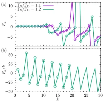
FIG. 1. Cumulant ratiosFk=ck+1/ck for time-independent test cases. The symbols are obtained with our propagation method, while the lines interpolate the results of the iteration scheme based on Eq. (11). (a) Asymmetric single-electron transistor for large bias and various dot-lead rates ΓS/D. (b) Triple quantum dot in ring configuration with ΓS = ΓD = 0.1∆, where dot 2 is detuned by = 10∆. For graphical reasons, we plotFk/k.

Despite the general validity of our formalism, in all ap- plications, we consider an array ofnquantum dots with the first dot coupled to an electron sourceS, while the last site is coupled to a drainD. Then the dot-lead tun- nelings can be written asL^dot-lead= ΓSD(c^†₁) + ΓDD(cn) with the Lindblad formD(x)ρ=xρx^†−¹2x^†xρ−¹2ρx^†x and the tunnel rates Γ_S/D. We evaluate the current at the source,` =S, such that the forward current opera- tor becomesJS⁺ρ≡ JS⁺= ΓSc^†₁ρc1, while the backward current operatorJS⁻ vanishes.

1. Single-electron transistor

One of the simplest transport setups is the single- electron transistor which consists of a resonant level be- tween two strongly biased leads. It can be occupied by at most one electron so that the Liouvillian and the forward current operator read

L=

−ΓS ΓD

ΓS −ΓD

, J⁺= 0 0

ΓS 0

, (13) respectively. For the symmetric case, ΓS = ΓD ≡ Γ, the cumulants of the single-electron transistor are known analytically asck = 2^−kΓ [14], which makes this system an ideal test case. Consequently, all cumulant ratiosFk = 1/2 are identical to the Fano factor. For any ΓS 6= ΓD, the cumulants cannot be written in a closed form, but

exhibit a generic behavior: While cumulants of low order reflect the nature of the transport process, high-order cumulants oscillate in a universal manner [27]. Therefore the symmetric case with its constantFk= 1/2 is rather special and should be sensitive to numerical errors.

By solving Eqs. (9) and (10) numerically, we have found that for ΓS = ΓD ≡ Γ, the first & 30 cumulant ratios agree with the analytical prediction with a pre- cision . 1% (not shown). For slight asymmetries, we compare in Fig. 1(a) our results with those obtained by the traditional iteration scheme. Both agree rather well also for orders at which the cumulants exhibit universal oscillations.

2. Triple quantum dot in a ring configuration As a further test case, we consider a ring of three quan- tum dots, where dots 1 and 3 are is coupled to source and drain, respectively, while dot 2 is detuned by a onsite en- ergy . The corresponding single-particle Hamiltonian reads

H =





0 ∆ ∆

∆ ∆

∆ ∆ 0



. (14) Transport may thus occur by direct tunneling from the first to the last dot or via dot 2. For strong detuning, ∆, the latter path has the effective tunnel matrix ele- ment ∆²/∆. Thus in the limit of strong Coulomb re- pulsion, the situation is that of a slow and a fast channel which block one another. This typically leads to bunch- ing visible in a super Poissonian Fano factor [15]. The triple quantum dot ring combines several difficulties such as different time scales, quantum interference, and cumu- lants that grow exponentially with their index [28]. The corresponding stiff differential equations represent chal- lenging test cases for propagation methods.

In Fig. 1(b) we again compare the results of our method with those of the iteration of Eq. (11). As for the double quantum dot, we find that for the first 20 cumulants, the results of both methods are practically indistinguishable. Owing to the mentioned difficulties, however, calculations for more than roughly 15 cumu- lants require a rather high numerical precision and, thus, are time consuming. Nevertheless, we can conclude that for the experimentally relevant orders, our scheme is still efficient and numerically stable.

IV. APPLICATIONS

To demonstrate the practical use of our time- dependent iteration scheme, we apply it to various phys- ical situations that have been studied recently, i.e., we generalize previous calculations of the current or the Fano factor to cumulants of higher order.

(a)

(b)

Ω12 Ω23

0 Ωmax

ck/Γ

t/T

c1 c2 c3 c4

−0.2

−0.1 0 0.1 0.2 0.3

0 2 4 6 8 10 12

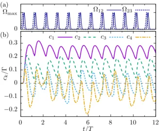
FIG. 2. (a) Pulsed tunnel matrix elements defined in Eq. (16) which lead to an adiabatic passage of electrons from dot 1 to dot 3. Each pulse has a width σ = T /16. The delay within a double pulse is ∆t =T /8, while the time between the pairs isT = 40/Ωmax. (b) Corresponding time evolution of the current cumulants ck, k = 1, . . . ,4, for the dot-lead rates ΓS= ΓD= 0.05Ωmax [29].

ck/Γ

ΩmaxT

¯ ρ2,2

c2

c3

c4

−0.6

−0.4

−0.2 0 0.2 0.4 0.6

20 40 60 80 100

FIG. 3. Time-averaged population of the central dot for steady-state CTAP as a function of the driving periodT to- gether with the cumulantsckfork= 2,3,4. All other param- eters are as in Fig. 2.

A. Steady-state coherent transfer by adiabatic passage

Let us consider a triple quantum dot described by the single-particle Hamiltonian

H(t) =





0 Ω12(t) 0 Ω12(t) 0 Ω23(t)

0 Ω23(t) 0



. (15) If the tunnel couplings Ωij are switched adiabatically slowly, the system may follow the adiabatic eigenstate

∝ (Ω23,0,−Ω12)^T. In this way, it is possible to trans- fer an electron from the first dot to the last dot without populating the middle dot [8], an effect known as CTAP.

This non-local version of an optical Lambda transition

[30] has also been predicted for atoms in multi-stable traps [9, 10].

Experimental evidence of the direct tunneling from the first to the last dot is hindered by the backaction of a population measurement, which creates decoherence [31] and, thus, may induce the effect that one wishes to demonstrate. To circumvent this problem, is has been suggested [7] to contact the triple quantum dot to an electron source and drain and to employ the sequence of double Gauss pulses

Ω12/23(t) =

∞

X

n=0

Ωmaxexph

−(t∓∆t/2−nT)² 2σ²

i (16)

with width σ, delay ∆t, and repetition time T, as is sketched in Fig. 2(a). Notice the so-called counter in- tuitive order of the pulses in which the tunnel matrix element Ω23 is active before Ω12. In the ideal case, this sequence will lead to the transport of one electron per double pulse and, thus, induce a current with a low Fano factor which may serve as experimental verification of CTAP.

While in Ref. [7] only the second current cumulant have been considered, we here focus on cumulants of higher or- der. We again assume that Coulomb repulsion inhibits the occupation with more than one electron. Then we have to add the empty state to the Hamiltonian (15), while the dissipative parts of the Liouville equation and the current operator remain the same as in the last sec- tion.

Figure 2(b) shows the time evolution of the first four current cumulants. After a transient stage of roughly 10T, the dynamics assumes its long time limit, from which we compute the steady state values of the cumu- lants as the average over the driving period. The time evolution illustrates that generally the duration of the transient stage increases with the cumulant order.

The central issue of verifying CTAP via noise measure- ments is the correlation between the Fano factor and the population of the middle dot as a function of the driving periodT. By contrast, the current correlates only weakly with the population and cannot serve as indicator [7].

Notice that a non-trivial value for the correlation coeffi- cient requires a non-monotonic variation of both curves, which indeed is the case. Going beyond this, we plot in Fig. 3 the corresponding cumulants of higher order aver- aged over one driving period in the long-time limit. We find that the third cumulant also correlates with the oc- cupation, while for the fourth cumulant only the absolute value behaves in this way. Interestingly enough, the pro- file ofc3andc4cumulant is even sharper than that of the zero-frequency noisec2 considered in Ref. [7]. Thus, the measurement of further cumulants will strengthen the ev- idence for the correct operation of a steady-state CTAP protocol.

(a)

(b)

(c)

A/Ω

0 2 4 6 8

0 0.2 0.4 0.6 0.8 1

I/Imax

A/Ω

0 2 4 6

0 0.2 0.4 0.6 0.8 1

S/Smax

A/Ω

0/Ω 0

2 4 6

−4 −3 −2 −1 0 1 2 3 4 0 0.2 0.4 0.6 0.8 1

F

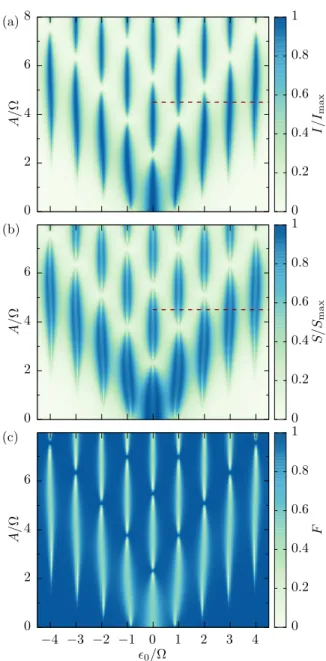
FIG. 4. Average currentc1 (a), zero-frequency noisec2 (b), and Fano factorc2/c1 (c) for a strongly biased driven double quantum dot as a function of the detuningand the driving amplitudeA. The driving frequency and the dot-lead tun- nel rates are Ω = 2∆ and ΓS = ΓD = 0.15∆, respectively.

The dashed horizontal lines mark the amplitude considered in Fig. 5.

B. Landau-Zener interference

A paradigmatic example for time-dependent quantum mechanics is a two-level system with the single-particle Hamiltonian

H(t) = 1 2

(t) ∆

∆ −(t)

, (17)

−0.1 0 0.1 0.2 0.3

0 1 2 3 4

ck/Γ

0/Ω

c1 c2 c3 c4

−0.1 0 0.1 0.2 0.3

0 1 2 3 4

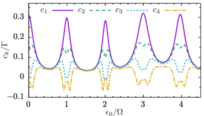
FIG. 5. First four cumulants ck for the LZSM interference patterns for the driving amplitude A = 4.5Ω marked in Fig. 4(a) by a horizontal line.

the tunnel matrix element ∆, and the time-dependent bias

(t) =0+Acos(Ωt). (18) For driving amplitudesA&0, the eigenenergies ofH(t) as a function of time form avoided crossings. At these crossings, an electron may perform Landau-Zener tran- sitions, such that repeated sweeps lead to the so-called LZSM interference. In a closed system, this is visible in a characteristic pattern of the population as a function of the detuning 0 and the amplitude A[32]. Having been measured originally for the population of superconduct- ing qubits [33, 34], such patterns have been found also for the current in a biased open double quantum dot [35, 36].

For deeper understanding, we extend previous results for the average current to a study of current cumulants.

Figure 4(a) shows the LZSM interference pattern for the time-averaged current, i.e., the first cumulantc1. It exhibits the typical structure found in the high-frequency limit, namely Lorentzian resonance peaks which by and large are modulated along the A-axis by the squares of Bessel functions [36]. For the second cumulant [Fig. 4(b)], the corresponding peaks split into double peaks whose local minima coincide with the current max- ima. As a consequence, the corresponding Fano fac- tor [Fig. 4(c)] assumes clearly sub Poissonian values of F1≈1/2, while off the resonance, the Fano factor indi- cates Poissonian transport.

For a closer and more quantitative investigation, we depict in Fig. 5 the first 4 cumulants as a function of the detuning 0 for constant driving amplitude. On the one hand, this highlights the double peak structure ofc2 and indicates that at the edge of the current peaks c2 ≈c1

which corresponds to the Poissonian F1 ≈1. The third and the fourth cumulants possess a similar double peak structure, where the magnitude of theckdiminishes with

the orderk. This affirms the low-noise properties of res- onantly driven transport in coupled quantum dots [37].

V. CONCLUSIONS

We have developed a method for the iterative com- putation of current cumulants for conductors described by a time-dependent Markovian master equation. For such transport problems the only generic way to ob- tain a solution is a numerical propagation while gener- ally eigenvalue-based methods are not applicable. Our scheme is based on a hierarchy of density operator like objects truncated according to desired number of cumu- lants. The cumulants follow in a direct manner by taking the trace. As compared to the propagation of a number- resolved density matrix, our scheme possesses two advan- tages. First, it generally gets along with a significantly smaller set of equations. Second, there is no need to compute the cumulants from the moments, a numerically critical task that may involve computing small differences of much larger numbers.

As a test bench, we have employed two time- independent master equations which can be solved also with previously known eigenvalue-based methods. This indicated that our scheme provides reliable results for roughly the first 10 cumulants even for challenging test cases. For less demanding situations, computing more than 30 cumulants is feasible. Thus, we reach orders way beyond the present experimental needs.

We have applied our scheme to two time-dependent systems of recent interest. For steady-state CTAP, we have found that not only the second cumulant, but also higher ones correlate with the population of the middle dot. Therefore they may provide additional evidence for the correct operation of a CTAP protocol. A similar conclusion can be drawn for Landau-Zener interference patterns of the current in open double quantum dots.

The higher-order cumulants substantiate the conclusions drawn from studies of the Fano factor.

In this spirit, our approach enables studies of the current noise for time-dependent transport beyond the second cumulant with a moderate computational effort.

This may provide additional insight to the underlying transport mechanisms and a deeper understanding of the electron dynamics controlled by arbitrarily shaped pulses.

ACKNOWLEDGMENTS

This work was supported by the Spanish Ministry of Economy and Competitiveness via Grant No. MAT2014- 58241-P and by the DFG via SFB 689.

[1] C. Beenakker and C. Sch¨onenberger, Phys. Today56(5), 37 (2003).

[2] Y. M. Blanter and M. B¨uttiker, Phys. Rep.336, 1 (2000).

[3] S. Camalet, J. Lehmann, S. Kohler, and P. H¨anggi, Phys.

Rev. Lett. 90, 210602 (2003).

[4] L. Fricke, M. Wulf, B. Kaestner, V. Kashcheyevs, J. Tim- oshenko, P. Nazarov, F. Hohls, P. Mirovsky, B. Mack- rodt, R. Dolata, T. Weimann, K. Pierz, and H. W. Schu- macher, Phys. Rev. Lett.110, 126803 (2013).

[5] B. Kaestner and V. Kashcheyevs, Rep. Prog. Phys.78, 103901 (2015).

[6] A. Croy and U. Saalmann, Phys. Rev. B 93, 165428 (2016).

[7] J. Huneke, G. Platero, and S. Kohler, Phys. Rev. Lett.

110, 036802 (2013).

[8] A. D. Greentree, J. H. Cole, A. R. Hamilton, and L. C. L.

Hollenberg, Phys. Rev. B70, 235317 (2004).

[9] K. Eckert, M. Lewenstein, R. Corbal´an, G. Birkl, W. Ert- mer, and J. Mompart, Phys. Rev. A70, 023606 (2004).

[10] R. Menchon-Enrich, A. Benseny, V. Ahufinger, A. D.

Greentree, Th. Busch, and J. Mompart, Rep. Prog. Phys.

79, 074401 (2016).

[11] D. K. C. MacDonald, Rep. Prog. Phys.12, 56 (1949).

[12] M. B¨uttiker, Phys. Rev. B46, 12485 (1992).

[13] L. S. Levitov and G. B. Lesovik, JETP Lett. 58, 230 (1993).

[14] D. A. Bagrets and Y. V. Nazarov, Phys. Rev. B 67, 085316 (2003).

[15] W. Belzig, Phys. Rev. B71, 161301(R) (2005).

[16] T. Brandes, Ann. Phys. (Leipzig)17, 477 (2008).

[17] C. Flindt, T. Novotn´y, A. Braggio, M. Sassetti, and A.- P. Jauho, Phys. Rev. Lett.100, 150601 (2008).

[18] C. Flindt, T. Novotn´y, A. Braggio, and A.-P. Jauho, Phys. Rev. B82, 155407 (2010).

[19] S. A. Gurvitz and Ya. S. Prager, Phys. Rev. B53, 15932 (1996).

[20] B. Kubala, J. Ankerhold, and A. D. Armour, ArXiv:

1606.02200.

[21] J. Cerrillo, M. Buser, and T. Brandes, ArXiv:

1606.05074.

[22] R. S´anchez, S. Kohler, and G. Platero, New J. Phys.10, 115013 (2008).

[23] N. G. van Kampen,Stochastic processes in physics and chemistry (North-Holland, Amsterdam, 1992).

[24] D. Darau, G. Begemann, A. Donarini, and M. Grifoni, Phys. Rev. B79, 235404 (2009).

[25] J. Koch and F. von Oppen, Phys. Rev. Lett.94, 206804 (2005).

[26] N. Lambert, F. Nori, and C. Flindt, Phys. Rev. Lett.

115, 216803 (2015).

[27] C. Flindt, C. Fricke, F. Hohls, T. Novotn´y, K. Netoˇcn´y, T. Brandes, and R. J. Haug, Proc. Natl. Acad. Sci. USA 106, 10116 (2009).

[28] F. Dom´ınguez, G. Platero, and S. Kohler, Chem. Phys.

375, 284 (2010).

[29] Notice that in the figures and captions of Ref. [7], all times should be multiplied by a factor 20, while the rates Γ andγ should be divided by 10.

[30] N. V. Vitanov, T. Halfmann, B. W. Shore, and K. Bergmann, Ann. Rev. Phys. Chem.52, 763 (2001).

[31] J. Rech and S. Kehrein, Phys. Rev. Lett. 106, 136808 (2011).

[32] S. N. Shevchenko, S. Ashhab, and F. Nori, Phys. Rep.

492, 1 (2010).

[33] W. D. Oliver, Y. Yu, J. C. Lee, K. K. Berggren, L. S.

Levitov, and T. P. Orlando, Science310, 1653 (2005).

[34] M. Sillanp¨a¨a, T. Lehtinen, A. Paila, Y. Makhlin, and P. Hakonen, Phys. Rev. Lett.96, 187002 (2006).

[35] J. Stehlik, Y. Dovzhenko, J. R. Petta, J. R. Johansson, F. Nori, H. Lu, and A. C. Gossard, Phys. Rev. B86, 121303(R) (2012).

[36] F. Forster, G. Petersen, S. Manus, P. H¨anggi, D. Schuh, W. Wegscheider, S. Kohler, and S. Ludwig, Phys. Rev.

Lett.112, 116803 (2014).

[37] M. Strass, P. H¨anggi, and S. Kohler, Phys. Rev. Lett.

95, 130601 (2005).