arXiv:1611.07210v1 [cond-mat.mes-hall] 22 Nov 2016

Spin-charge coupling effects in a two-dimensional electron gas

Roberto Raimondi

Dipartimento di Matematica e Fisica, Universit`a Roma Tre, Via della Vasca Navale 84, Rome, 00146, Italy

E-mail: roberto.raimondi@uniroma3.it www.uniroma3.it

Cosimo Gorini

Institut f¨ur Theoretische Physik, Universit¨at Regensburg, 93040 Regensburg, Germany

E-mail: cosimo.gorini@physik.uni-regensburg.de

Sebastian T¨olle

Institut f¨ur Physik, Universit¨at Augsburg Universit¨atsstr. 1, 86135 Augsburg, Germany E-mail: sebastian.toelle@physik.uni-augsburg.de

In these lecture notes we study the disordered two-dimensional electron gas in the presence of Rashba spin-orbit coupling, by using the Keldysh non- equilibrium Green function technique. We describe the effects of the spin-orbit coupling in terms of a SU(2) gauge field and derive a generalized Boltzmann equation for the charge and spin distribution functions. We then apply the formalism to discuss the spin Hall and the inverse spin galvanic (Edelstein) ef- fects. Successively we show how to include, within the generalized Boltzmann equation, the side jump, the skew scattering and the spin current swapping processes originating from the extrinsic spin-orbit coupling due to impurity scattering.

Keywords: Spin-orbit coupling; Electronic transport; Many-body Green func- tion; Disordered systems.

1. Introduction

These lecture notes are based mainly on the work by Gorini et al. of Ref. 1, where by means of a gradient expansion a generalized Boltzmann equation with SU(2) gauge fields was obtained for the disordered Rashba model. The inclusion of the extrinsic spin-orbit coupling (SOC) from impurities in the SU(2) formalism was later considered in the work by Raimondi et al. in Ref.

2. Hence, the aim of these lecture notes is to provide a self-contained and

arXiv:1611.07210v1 [cond-mat.mes-hall] 22 Nov 2016

pedagogical introduction to the disordered two-dimensional electron gas (2DEG) with both intrinsic (Rashba) and extrinsic SOC within the SU(2) gauge-field approach. The lecture notes by Tatara in this series are a good complementary reading dealing with electron transport in ferromagnetic metals³.

The layout of these lecture notes is the following. In Section 2 we write down the quantum kinetic equation for the fermion Green function in the presence of U(1), associated with the electromagnetic field, and SU(2) gauge fields.

The standard model of disorder is introduced in Section 3. Whereas in Section 2 we derive the hydrodynamic SU(2) derivative of the Boltzmann equation, in Section 3 we obtain an expression for the collision integral describing the scattering from impurities. In Section 4 we apply the for- malism to the disordered Rashba model and derive the Bloch equation for the spin density, describe the Dyakonov-Perel spin relaxation, and discuss a thermally induced spin polarization. In Section 5 we introduce SOC from impurity scattering and analyze the so-called side jump mechanism, which manifests as a correction to the velocity operator. In Section 6 we discuss the skew scattering mechanism. Both intrinsic and extrinsic SOCs con- tribute to the spin relaxation. Extrinsic SOC gives rise to Elliott-Yafet spin relaxation, which is covered in Section 7, together with the complete form of the Boltzmann equation. Section 8 states our conclusions. Throughout we use units such that ~=c= 1.

2. The kinetic equation and the SU(2) covariant Green function

We begin by defining the Keldysh Green function (for an introduction see, e.g., the book by Rammer⁴)

Gˇ =

G^RG^K 0 G^A

, (1)

where the retarded G^R, Keldysh G^K and advanced G^A components are given by

G^R(r1, t1;r2, t2) =−iΘ(t1−t2)hψ(r1, t1)ψ^†(r2, t2) +ψ^†(r2, t2)ψ(r1, t1)i G^K(r1, t1;r2, t2) =−ihψ(r1, t1)ψ^†(r2, t2)−ψ^†(r2, t2)ψ(r1, t1)i

G^A(r1, t1;r2, t2) =iΘ(t2−t1)hψ(r1, t1)ψ^†(r2, t2) +ψ^†(r2, t2)ψ(r1, t1)i. In the above definitionsψ(r1, t1) andψ^†(r2, t2) are Heisenberg field opera- tors for fermions and Θ(t) the Heaviside step function. In the following we

will be concerned with spin one-half fermions. As a consequence, all entries of ˇGbecome two by two matrices.

To derive a kinetic equation, it is useful to introduce Wigner mixed coor- dinates. To this end we perform a Fourier transform with respect to both space (r1−r2) and time (t1−t2) relative coordinates

G(p, ;ˇ r, t) = Z

d(t1−t2) Z

d(r1−r2) ˇG(r1, t1;r2, t2)e^{i[(t1−t2)−p·(r1−r2)]}. (2) The first step in the standard derivation of the kinetic equation is the left- right subtracted Dyson equation

Gˇ⁻¹₀ (x₁, x₃)^⊗,Gˇ(x₃, x₂)

= 0, (3)

where we have used space-time coordinates x1 ≡(r1, t1) etc. In Eq. (3), the symbol ⊗ implies integration overx₃ and matrix multiplication both in Keldysh and spin (if any) spaces. Furthermore

Gˇ⁻¹₀ (x1, x₃) = (i∂t1−H)δ(x1−x₃), (4) where H is the Hamiltonian operator. In these lecture notes we do not consider electron-electron interaction. Quite generally the Hamiltonian op- erator takes the form

H= (−i∇^r+eA(r, t))²

2m −eΦ(r, t) +V(r). (5) Here e=|e|and we have assumed negatively charged particles. In Eq. (5) the scalar and vector potential have a two by two matrix structure, which can be shown by expanding them in the basis of the Pauli matrices

Φ = Φ⁰σ⁰+ Φ^aσ^a

2 , A=A⁰σ⁰+A^aσ^a

2 , a=x, y, z, (6) and summation over the repeated indices is understood. The σ⁰- components are the electromagnetic scalar and vector potentials associated with the U(1) gauge invariance. V(r) describes the disorder potential due to impurities and defects. In this section we set V(r) = 0 and postpone its discussion to the following section. The σ^a-components are an SU(2) gauge field, whose scalar and vector components can be used to respectively describe a Zeeman/exchange term and SOC – in our case Rashba SOC, as will be shown in Sec. 4. For the time being, we do not consider a specific form of the SU(2) gauge field (Φ^a,A^a).

The goal of a kinetic equation is to describe non-equilibrium phenomena.

In general this is a formidable task. However, for close-to-equilibrium phe- nomena or for non-equilibrium ones occurring on scales large compared to

microscopic ones, it is possible to derive an effective kinetic equation by means of the so-called gradient expansion. The idea is based on the obser- vation that under specific circumstances the Green function varies fast with respect to the relative coordinatex1−x2and much more slowly with respect to the center-of-mass one (x1+x2)/2. In equilibrium, for a translationally invariant system, the Green function does not depend on the center-of-mass coordinate at all.

To understand how the gradient expansion works, consider the convolution of two quantities

(A⊗B)(x1, x2) = Z

dx3A(x1, x3)B(x3, x2),

which can be equivalently expressed as a function of center-of-mass and relative coordinates

Z dx3A

x1+x3

2 , x1−x3

B

x3+x2

2 , x3−x2

.

Next, replacex1+x3=x1+x2+x3−x2andx3+x2=x1+x2−(x1−x3) in the first argument ofAandB, respectively. By Taylor expandingAwith respect tox3−x2 in its first argument andB with respect tox1−x3 in its first argument, after Fourier transforming according to Eq. (2), one gets

A(x, p)B(x, p) +i

2 ∂µA(x, p)

∂_p^µB(x, p)

−i

2 ∂_p^µA(x, p)

∂µB(x, p) , (7) where we have introduced the compact (relativistic) space-time notations

x^µ = (t,r), xµ= (−t,r), p^µ= (,p), pµ= (−,p) (8) and

∂^µ≡ ∂

∂x_µ, ∂_µ≡ ∂

∂x^µ, ∂_p^µ≡ ∂

∂p_µ, ∂_p,µ≡ ∂

∂p^µ (9)

in a such a way that the productp^µxµ=−t+p·rhas the correct Lorentz metrics. Equation (3) acquires then the form

−iGˇ⁻¹₀ ,Gˇ +1

2

∂^µGˇ⁻¹₀

, ∂p,µGˇ −1 2

∂^µ_pGˇ⁻¹₀

, ∂µGˇ = 0. (10) The Hamiltonian (5) is invariant under a gauge transformationO(x), which locally rotates the spinor field

ψ⁰(x) =O(x)ψ(x), ψ^0†(x) =ψ^†(x)O^†(x), O(x)O^†(x) = 1. (11) The Green function, however, is not locally covariant, i.e. its transformation depends on two distinct space-time points

G(xˇ 1, x₂)→O(x1) ˇG(x1, x₂)O^†(x2). (12)

Physical observables, which are locally covariant, are obtained by consid- ering the Green function in the limit of coinciding space-time points. It is then useful to introduce a locallycovariant Green function

ˇ˜

G(x1, x₂) =U_Γ(x, x1) ˇG(x1, x₂)UΓ(x2, x) (13) where

UΓ(x, x1) =Pexp

−i Z x

x1

eA^µ(y)dyµ

. (14)

The line integral of the gauge field is referred to as the Wilson line. In Eq. (14) P is a path-ordering operator and A^µ = (Φ,A), A_µ = (−Φ,A).

Since the Wilson line transforms covariantly

U_Γ(x, x1)→O(x)UΓ(x, x1)O^†(x1), (15) one easily sees that the covariant Green function ˇ˜Gtransforms in a locally covariant way

G(xˇ˜ 1, x2)→O(x) ˇ˜G(x1, x2)O^†(x). (16) When x₁ = x₂ = x, the locally covariant Green function coincides with the original Green function. By inverting Eq. (13), one can, via Eq. (10), obtain an equation for the locally covariant Green function. Due to the non-Abelian character of the gauge field, Eq. (13) is not easy to handle.

In the spirit of the gradient approximation, we assume that ∂^µ∂µ,p 1.

In addition we also assume that eA^µ∂µ,p 1. This assumption can be justified on physical grounds once an explicit form is assigned toA. Under these assumptions, Eq. (13) becomes

Gˇ˜= ˇG−1

2{eA^µ∂_p,µ,Gˇ} (17) and its inverse

Gˇ= ˇ˜G+1

2{eA^µ∂p,µ,Gˇ˜}. (18) By using the decomposition

δ(x1−x₂) =

Z d^d+1p

(2π)^d+1e^{ipµ(x1,µ−x2,µ)}, (19) one obtains

Gˇ⁻¹₀ (x, p) =−(p+eA(x))²

2m +eΦ(x) =− p²

2m−V^µeAµ−e²A² 2m , (20)

from which

∂_p^µGˇ⁻¹₀ (x, p) =−V^µ− ∂^µ_pV^ν eA_ν,

∂^µGˇ⁻¹₀ (x, p) =−V^ν∂^µeAν. (21) In the above V^µ = (1,p/m) is thed-current operator, dbeing the space dimensionality. In the second equation of (21) we neglected the term

∂^µe²A²/2m=eA·∂^µeA because it gives a small correction top·∂^µeA when p∼p_F. Performing theshifttransformation of Eq. (17) in Eq. (20) gives

ˇ˜

G⁻¹₀ =− p²

2m. (22)

We have now all the necessary ingredients to obtain the equation for ˇ˜G.

We begin by considering the first term of Eq. (10). By applying the shift transformation of Eq. (17) and expressing ˇGin terms of ˇ˜Gvia Eq. (18), we obtain

−i h

Gˇ⁻¹₀ ,Gˇ˜i

−1 2 n

eAµ, ∂_p^µh

Gˇ⁻¹₀ ,Gˇ˜i o +1

2

hGˇ⁻¹₀ ,n

eAµ, ∂_p^µGˇ˜oi . (23) By means of the identity {A,[B, C]} −[B,{A, C}] ={[A, B], C}we get

ieV^µ h

A_µ,Gˇ˜i +1

2

ne[A_µ, A_ν], ∂^ν_pGˇ˜o

. (24)

As for the second term of Eq. (10) 1

2

∂^µGˇ⁻¹₀

, ∂_p,µGˇ → −e 2V^µn

(∂^νA_µ), ∂_p,νGˇ˜o

, (25)

where the last step follows by considering the first order of the gradient expansion. Finally, for the last term of Eq. (10)

−1 2

∂_p^µGˇ⁻¹₀

, ∂µGˇ →V^µ

∂µGˇ˜+1 2

n(e∂µA^ν), ∂p,νGˇ˜o

, (26) where we omitted terms ∼ ∂µ∂_p^νGˇ˜ within the first order accuracy of the gradient expansion. By collecting the results of Eqs.(24-26), the equation for ˇ˜Greads

V^µ

∂˜µGˇ˜+1 2

n

eFµν, ∂_p^νGˇ˜o

= 0, (27)

where we have introduced the covariant derivative

∂˜µGˇ˜=∂µGˇ˜+ih

eAµ,Gˇ˜i

(28)

and the field strength

F_µν =∂_µA_ν−∂_νA_µ+ie[A_µ, A_ν]. (29) It is useful at this stage to separate the space and time parts and rewrite Eq. (27) as

∂˜t+ p

m ·∇˜^rGˇ˜−e 2

np

m·E, ∂Gˇ˜o +1

2 n

F,∇^pGˇ˜o

= 0, (30) where the generalized Lorentz force reads

F=−e E+ p

m ×B

(31) with the U(1)×SU(2) fields given by

E=−∂tA− ∇^rΦ +ie[Φ,A], Bi = 1

2εijkF^jk. (32)

Equation (30) is the quantum kinetic equation. One can integrate over the energy , corresponding to the equal-time limit, in order to obtain a semiclassical kinetic equation. We define the distribution function as

f(p,r, t)≡1 2

1 +

Z d

2πiG˜^K(p, ;r, t)

, (33)

which is a matrix in spin space, f =f⁰σ⁰+f^aσ^a, a=x, y, z. By taking the Keldysh component of Eq. (30) we get

∂˜t+ p m·∇˜^r

f(p,r, t) +1 2 n

F· ∇^p, f(p,r, t)o

= 0. (34)

We have then obtained a generalization of the Boltzmann equation, where space and time derivatives are replaced by the covariant ones and the gen- eralized Lorentz force appears. We may then introduce the density and current by integrating over the momentum

ρ(r, t) =X

p

f(p,r, t), J(r, t) =X

p

p

mf(p,r, t). (35) Hence the integration over the momentum of Eq. (34) leads to a continuity- like equation

∂˜tρ(r, t) + ˜∇^r·J(r, t) = 0. (36) We will use the above equation in Section 4, when discussing the spin Hall and inverse spin galvanic/Edelstein effects in the Rashba model.

3. The standard model of disorder and the diffusive approximation

In this section we consider the effect of disorder due to impurity scattering.

According to the standard model of disorder⁵the potentialV(r) is assumed to be a random variable with distribution

hV(r)i= 0, hV(r)V(r⁰)i=n_iv²₀δ(r−r⁰). (37) In the aboveni is the impurity density andv0is the scattering amplitude.

Higher momenta can be present, and indeed they will be needed when considering skew-scattering processes, but it is not necessary to specify them for the time being. Disorder effects can be taken into account in perturbation theory via the inclusion of a self-energy. Equation (3) becomes

Gˇ⁻¹₀ (x1, x₃)^⊗,G(xˇ 3, x₂)

=Σ(xˇ 1, x₃)^⊗,G(xˇ 3, x₂)

. (38)

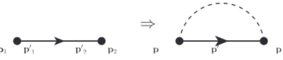
The lowest order self-energy due to disorder is given in Fig. 1 and its ex- pression reads

Σˇ0(p, x) =n_iv²₀X

p⁰

G(p, x).ˇ (39)

Notice that the integration is only on the space component of the d- momentum p^µ = (,p⁰). This is a result of the fact that the scattering is elastic. In order to use the above self-energy, we must transform it to the locally covariant formalism according to the transformation of Eq. (17) and express ˇGin terms of ˇ˜Gvia Eq. (18). This procedure is the same we have followed in the previous section to transform the kinetic equation from the form of Eq. (10) to the form Eq. (27). Since the procedure will also be used later on, let us show it in detail in this simple case. First we notice that

UΓ(x, x1)Σ(xˇ 1, x3)^⊗,G(xˇ 3, x2)

UΓ(x2, x) =h

ˇ˜Σ(x1, x3)^⊗,G(xˇ˜ 3, x2)i (40) after using the unitarity of the Wilson line by inserting

UΓ(x3, x)UΓ(x, x3) = 1

between the self-energy and the Green function. The locally covariant self- energy reads

ˇ˜Σ0=n_iv²₀X

p⁰

Gˇ˜_p⁰+1 2 n

A^µ(∂p⁰,µ−∂_p,µ),Gˇ˜_p⁰o

=n_iv₀²X

p⁰

Gˇ˜_p⁰. (41)

In the above the derivative with respect tocancels in the two terms. The derivative with respect to p vanishes because there is no dependence on

p. Finally, the derivative with respect to p⁰ can be integrated giving at most a constant, which can be discarded. As a result, the locally covariant self-energy has the same functional form of the original self-energy. The

p

p1 p^′1 p^′2 p2 p p^′ p

⇒

Fig. 1. Self-energy diagram to second order in the impurity potential (black dot vertex).

The diagram on the left is before the impurity average, which is carried in the diagram on the right as a dashed line connecting the two impurity insertions. Notice that the impurity average in momentum space yieldshV(p1−p⁰₁)V(p⁰₂−p2)i=niv₀²δ(p1−p⁰₁+ p⁰₂−p2).

Keldysh component of the collision integral then reads I˜=−ih

ˇ˜Σ,Gˇ˜p

i^K

=−iniv²₀X

p⁰

( ˜G^R_p0−G˜^A_p0) ˜G^K_p −( ˜G^R_p−G˜^A_p) ˜G^K_p0

. (42) Note that the SU(2) shifted retarded and advanced Green functions have no spin structure and therefore commute with the Keldysh Green function.

For weak scattering, one can ignore the broadening of the energy levels in the retarded and advanced Green function and use

G˜^R_p−G˜^A_p=−2πiδ(−p), G˜^K_p =−2πiδ(−p)(1−2f(p,r, t)). (43) As a result, Eq. (34) is no longer collisionless and becomes

∂˜t+ p m·∇˜^r

f(p,r, t)−e 2

n E+ p

m×B

· ∇^p, f(p,r, t)o

=I[f], (44) with the collision integral being

I[f] =−2πniv²₀X

p⁰

δ(p−p⁰)(f(p,r, t)−f(p⁰,r, t)). (45) It is appropriate in the final part of this section to obtain the solution of the Boltzmann equation Eq. (44) in the diffusive approximation. First we notice that, by integration over the momentump, the collision integralIvanishes reproducing the continuity equation (36) with density and current defined in Eq. (35). In the diffusive approximation we expand the distribution function in spherical harmonics

f(p,r, t) =hfi+ 2ˆp·f +. . . (46)

and keep terms up to the p-wave symmetry. In the above h. . .iindicates the integration over the directions of the momentum. We perform the evaluation in two space dimensions having in mind the application of the theory to the 2DEG. By defining the momentum relaxation time^a

1

τ = 2πN0niv²₀ (47)

with the density of statesN0=m/(2π) the collision integral becomes I[f] =−1

τ2ˆp·f. (48)

In the diffusive approximation we considerωτ 1 andvFqτ 1, whereω andqare typical energy and momentum scales. For instance,ω can be the magnitude of an externally applied magnetic field. We multiply Eq. (44) by ˆpand integrate over the angleφwith ˆp= (cosφ,sinφ). We get

−1 τf = p

2m∇˜^rhfi−e 2hn

ˆ

pE·∇^p,hfio i− e

2mhn ˆ

p(p×B·∇^p),2ˆp·fo i. (49) The first term, keeping in mind Eq. (35) for the current, represents the diffusivecontribution including the additional part due to the SU(2) gauge field. Due to the covariant nature of the derivative, such a term differs from zero even in uniform circumstances. The second term yields the usualdrift contribution, whereas the third one gives rise to a Hall contribution. The gradient with respect to the momentum can be split as∇^p= ˆp∂_p−φ∂ˆ _φ/p where ˆφ= (−sinφ,cosφ). Then we get

f =−τ p

2m∇˜^rhfi+eτ 4

n

E, ∂phfio + eτ

2m n

B×,fo

. (50)

By using the definitions of density and current in Eq. (36), we may write the expression for the number and spin components as

n= Tr [ρ], J⁰= Tr [J], s^a= 1

2Tr [σ^aρ], J^a =1

2Tr [σ^aJ]. (51) To begin with, let us consider the drift term

Jdr=X

p

p m

eτ 4

n

E, ∂phfio

=eN0

Z

dpD(p)1 2 n

∂_phfi,Eo

=−e 2

nσ(µ),Eo

(52) wherep=p²/2m,D(p) =τ p/m,µ=ρ/N0is a spin-dependent chemical potential, andσ(µ) =N0D(µ). In equilibrium,ρeq =N0F +N0Φ and its

aIts expression can also be obtained, for instance, by the Fermi golden rule.

eigenvalues determine the chemical potentials for up and down electrons.

Then

J⁰_dr=−eN₀D⁰E⁰−e

2N₀D^aE^a, J^a_dr=−e

4N₀D⁰E^a−e

2N₀D^aE⁰, (53) withD⁰ andD^a defined byD(µ) =D⁰+D^aσ^a. By expanding aroundF, one has D⁰≈D(F) andD^a ≈τ s^a/(N0m), and therefore

σ(µ) =N₀D(F)σ⁰+ τ

ms^aσ^a. (54)

The diffusion term is obtained by integrating over the momentum the first term of Eq. (50)

Jdif =−N0

Z

dpD(p) ˜∇^rhfi=−1 2

nD(µ),∇˜^rρo

. (55)

The above form of the diffusion term is determined by requiring that in equilibrium it must cancel the drift term according to the Einstein argu- ment. Then

J⁰_dif =−D⁰∇^rn−2D^ah

∇˜^rsi^a

, J^a_dif =−1

2D^a∇^rn−D⁰h

∇˜^rsi^a

. (56) Finally the Hall term yields

J⁰_Hall= eτ

mB⁰×J⁰+eτ

mB^a×J^a, J^a_Hall=eτ

mB⁰×J^a+ eτ

4mB^a×J⁰. (57) To summarize, we may write the particle and spin currents as

J⁰=−eN0D⁰E⁰−e

2N0D^aE^a−D⁰∇^rn−2D^ah

∇˜^rsi^a + eτ

mB⁰×J⁰+eτ

mB^a×J^a (58)

and

J^a=−e

4N₀D⁰E^a−e

2N₀D^aE⁰−1

2D^a∇^rn−D⁰h

∇˜^rsi^a + eτ

mB⁰×J^a+ eτ

4mB^a×J⁰. (59)

The above two equations, together with the continuity-like Eq. (36), will be used in the next section to analyze the spin Hall and Edelstein effect in the disordered Rashba model.

4. The disordered Rashba model The Rashba Hamiltonian reads⁶

H = p²

2m+αpyσ^x−αpxσ^y. (60) The only non zero components of the SU(2) gauge field are

eA^y_x=−2mα, eA^x_y= 2mα. (61) As shown in the previous sections (cf. Eq. (36)), the spin density obeys a continuity-like equation

∂˜_ts^a+ ˜∇^r·J^a = 0, (62) which is deceptively simple. The notable fact in the present theory is that the covariant derivatives defined in Eq. (28) appear also at the level of the effective phenomenological equations, providing an elegant and compact way to derive the equation of motion for the spin density. The explicit ex- pressions of the space and time covariant derivatives of a generic observable O^a read^b

∂˜tO^a =∂tO^a+abc eΦ^bO^c (63)

∇˜ⁱO^a =∇ⁱO^a−_abc eA^b_iO^c. (64) Equation (62) becomes

∂ts^a+abc eΦ^bs^c+∇ⁱJ_i^a−abc eA^b_iJ_i^c= 0, (65) showing that the equation for the spin is not a simple continuity equation, as expected from the non conservation of spin. The second term in Eq. (65) is the standardprecessionterm. The last term of (65) can be made explicit by providing the expression for the spin current J_i^a, where the lower (upper) index indicates the space (spin) component. The expression of J_i^a was derived via a microscopic theory in the diffusive regime in Eq. (59). The explicit expression reads

J_i^a =−eτ

ms^aEi+DabceA^b_is^c− eτ

4mijkJj B_k^a−eDN₀

2 E_i^a, (66) where D =D(F) is the diffusion constant. Let us apply Eqs. (65-66) to the Rashba model defined by Eq. (61) in the presence of an applied electric field along the x directionEx. To linear order in the electric field, the first term of Eq. (66) does not contribute in a paramagnetic system. Also by

b_abcis the fully antisymmetric Ricci tensor.

using Eq. (61) in the expressions of the fields of Eq. (32) we get that the SU(2) electric field vanishesE_i^a = 0 and that the only non zero component of the SU(2) magnetic field reads

eB^z_z=−(2mα)². (67)

Because the electric field is uniform, we may ignore the space derivative and obtain the explicit form of Eq. (65)

∂ts^x=−2mαJ_x^z (68)

∂ts^y=−2mαJ_y^z (69)

∂ts^z= +2mαJ_y^y+ 2mαJ_x^x (70) with the associated expressions for the spin currents

J_x^z = 2mαDs^x (71)

J_y^z = 2mαDs^y+θ_SH^intJ_x⁰ (72)

J_x^x=J_y^y =−2mαDs^z, (73)

whereJ_x⁰=−eσ(F)Exis the charge current andθ_SH^int is the spin Hall angle for intrinsic SOC

θ^int_SH=−mτ α². (74) Insertion of Eqs. (71-73) into (68-70) gives the Bloch equations

∂ts^x=− 1 τDP

s^x (75)

∂ts^y =− 1

τ_DP(s^y−s0) (76)

∂_ts^z =− 2

τ_DPs^x (77)

where the Dyakonov-Perel relaxation time is given by

τ_DP⁻¹ = (2mα)²D (78)

and the current-induced spin polarization is given by

s0=−eN0ατ Ex. (79) In the static limit the solution of the Bloch equations yields an in-plane spin polarization perpendicular to the electric field s^y =s⁰, withs^x =s^z = 0.

This is known as the Edelstein^7,8 or inverse spin-galvanic effect^9,10. The vanishing of the time derivative implies, via Eq. (69), the vanishing of the spin current J_y^z associated to the spin Hall effect. This vanishing occurs

thanks to the exact compensation of the two contributions appearing in Eq. (72). ^c

The above analysis can be extended in the presence of a thermal gradient.

More precisely, we derives^yin terms of a stationary thermal gradient along thex-direction,∇^xT, in the absence of any additional external fields.¹² However, in an experiment one would still measure an electric fieldE_xdue to a gradient in the chemical potential, ∇^xµ, resulting from an imbalance of the charge carriers due to the thermal gradient. For this, we shall first consider the trace of Eq. (50):

f⁰=−τ p

2m∇hf⁰i, (80)

where we can approximate∇hf⁰ias the Fermi functionf^eq, giving us f_x⁰=−τ p

2m −µ

T ∇^xT+∇^xµ −∂f^eq

∂

(81) for thex-component of Eq. (80). With use of the Sommerfeld expansion

Z dg()

−∂f^eq

∂

=g(µ) +π²

6 (kBT)² ∂²g

∂² _=µ

, (82)

where g() is an arbitrary energy dependent function, we end up with the particle current in the x-direction as follows:

J_x⁰=−2τ N₀ m

π² 3

(k_BT)²

T ∇^xT+µ∇^xµ

. (83)

We shall consider an open circuit alongx-direction, i.e., a vanishing particle currentJ_x⁰= 0. Then, we can express the electric field one would measure in an experiment as

E_x=1

e∇^xµ=S∇^xT, (84) where S =−(πkB)²T /(3eµ) is the Seebeck coefficient. After having ana- lyzed the charge sector, we consider next the spin sector in order to get an expression for s^y. We start by multiplying Eq. (50) with σ^z and perform the trace. They-component reads

f_y^z= 2pτ αhf^yi+eτ

mB_z^zf_x⁰. (85)

cTo make contact with the diagrammatic Kubo formula approach, we notice that the second term of Eq. (72) corresponds to a bubble-like diagram, whereas the first term describes the so-called vertex corrections.¹¹

Note that the form of Eq. (69) doesn’t change and since we assume a sta- tionary case we have

J_y^z= 0⇔f_y^z= 0. (86) This implies that there is no spin Nernst effect as no spin Hall effect in the disordered Rashba model. From Eq. (85), together with Eq. (81) we therefore find

hf^yi= 2αm

p f_x⁰=−ατ −µ

T ∇^xT+∇^xµ −∂f^eq

∂

. (87) From the form of the latter equation and with use of the Sommerfeld ex- pansion, Eq. (82), it is clear that we can express the y spin polarization as

s^y =PsT∇^xT+PsEEx, (88) where PsT can be written in a Mott-like form:

PsT =−Sµ∂PsE

∂µ . (89)

Here, we find PsE =−ατ eN0, consistent with Eq. (76). This results in a vanishing P_sT since P_sE is independent of µ. We express E_x in terms of

∇^xT with use of Eq. (84) and end up with

s^y=−ατ eN₀S∇^xT, (90) describing the thermal Edelstein effect in the disordered Rashba model.

5. The impurity-induced spin-orbit coupling: swapping and side jump mechanisms

In this and following sections we consider theextrinsicSOC due to impurity scattering described by the Hamiltonian

H_ext,so=−λ²₀

4 σ× ∇V(r)·p, (91) where λ₀ is the effective Compton wave length^13,14. In developing the perturbation theory in the impurity potential we must now use the lowest order scattering amplitude

Sp⁰,p⁰⁰ =Vp⁰−p⁰⁰

1−iλ²₀

4 p⁰×p⁰⁰·σ

(92) with

hV_q1V_q2i=n_iv₀²δ(q1+q₂). (93)

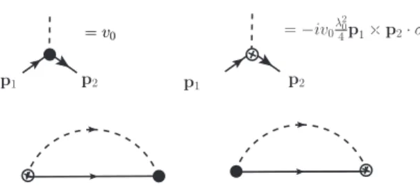
=v₀

=v₀ =−iv₀^λ₄²⁰p₁×p₂·σ

p₁ p₂ p₁ p₂

Fig. 2. In the top line the impurity insertion without (black dot vertex) and with (crossed dot vertex) spin-orbit coupling. In the bottom line the two diagrams to first order in the spin-orbit couplingλ²₀.

To zeroth order in λ²₀, we have the diagram of Fig. 1, which has been studied in the previous section. To first order in λ²₀, we must consider the two diagrams of Fig. 2. Here an empty crossed dot stands for the part of the scattering amplitude with the spin-orbit coupling. Let us evaluate these diagrams step by step. Before the impurity average (indicated as h. . .i), the expression for the two diagrams reads

Σˇ1,p⁰,p⁰⁰ =−iλ²₀ 4

X

p₁,p₂

hVp⁰−p1 p⁰×p1·σGˇp₁,p₂

+ ˇGp₁,p₂p2×p⁰⁰·σ

Vp₂−p⁰⁰i. (94) In the above, ˇGp₁,p₂ is the Fourier transform with respect to the space arguments r₁ and r₂ of ˇG(r1,r₂). We do not mention explicitly here the time arguments for the sake of simplicity. Performing the impurity average one obtainsp⁰−p1=p⁰⁰−p2. It is convenient then to define momenta as

p= p⁰+p⁰⁰

2 , q=p⁰−p⁰⁰=p1−p2, p˜= p₁+p₂

2 (95)

in such a way that p and ˜p correspond to the momentum of the mixed Wigner representation introduced previously. The momentum q instead is the variable conjugated to the center-of-mass coordinate r by Fourier transform. We then get the impurity-averaged expression of the two first- order diagrams

Σˇ1(p,q) =−iλ²₀

4 n_iv₀²X

˜ p

hp+q 2

×

˜ p+q

2

·σGˇ(˜p,q)

+ ˇG(˜p,q)

˜ p−q

2 ×

p−q 2

·σi

. (96)

The above expression can be divided into three terms Σˇ1,a(p,q)) =−iλ²₀

4 n_iv²₀X

˜ p

p×p˜·σ,G(˜ˇ p,q)

(97) Σˇ1,b(p,q)) =−iλ²₀

8 niv²₀X

˜ p

n

p×q·σ,G(˜ˇ p,q)o

(98) Σˇ1,c(p,q)) =iλ²₀

8 niv₀²X

˜ p

np˜×q·σ,G(˜ˇ p,q)o

. (99)

One can Fourier transform back to the center-of-mass coordinate r and re-label ˜p→p⁰

Σˇ1,a(p,r)) =−iλ²₀

4 niv₀²X

p⁰

p×p⁰·σ,G(pˇ ⁰,r)

(100) Σˇ1,b(p,r)) =−∇^r·λ²₀

8 n_iv²₀X

p⁰

nσ×p,Gˇ(p⁰,r)o

(101) Σˇ1,c(p,r)) =∇^r· λ²₀

8 niv₀²X

p⁰

n

σ×p⁰,G(pˇ ⁰,r)o

. (102)

Equations (100-102) are the final expression for the diagrams of the second line of Fig. 2. The first term ˇΣ1,a, as we will see, describes the swapping of spin currents under scattering¹⁵. The other two terms, ˇΣ1,b and ˇΣ1,c, are written as a divergence. As a consequence, when they are inserted in the collision integral of the kinetic equation, they lead to a correction of the velocity operator and hence describe the so-called side-jumpmechanism¹⁶. Until now we have not yet considered the effect of the gauge fields on the extrinsic SOC. To do it, we must transform the above derived self-energy to the locally covariant form. Let us first examine the U(1) gauge field corresponding to a static electric field E⁰ =−∇^rΦ⁰(r). The shift of the gradient of the Green function yields

∇^r^G(p,ˇ r) =∇^rG(p,ˇ r)−1 2

neΦ⁰∂,∇^rG(p,ˇ r)o

=∇^rG(p,ˇ˜ r) +1 2∇^rn

eΦ⁰∂,G(p,ˇ˜ r)o

−1 2

neΦ⁰∂,∇^rG(p,ˇ˜ r)o

=∇^rG(p,ˇ˜ r)−eE⁰∂G(p,ˇ˜ r). (103)

As a result we get from Eqs.(101-102) two more terms δΣˇ1,b(p,r)) =eE⁰· λ²₀

8 niv₀²X

p⁰

n

σ×p, ∂G(pˇ˜ ⁰,r)o

(104)

δΣˇ1,c(p,r)) =−eE⁰·λ²₀

8 n_iv²₀X

p⁰

nσ×p⁰, ∂Gˇ˜(p⁰,r)o

. (105) Let us transform Eq. (100) to the locally covariant form

ˇ˜

Σ1,a(p,r) =−iλ²₀

4 niv²₀X

p⁰

h

p×p⁰·σ,G(pˇ˜ ⁰,r)i +iλ²₀

4 n_iv₀²X

p⁰

1 2

hp×p⁰·σ,n

eA· ∇^p0,G(pˇ˜ ⁰,r)oi

−iλ²₀

4 niv₀²X

p⁰

1 2 n

eA· ∇^p,h

p×p⁰·σ,G(pˇ˜ ⁰,r)i o ,

which can be rewritten as ˇ˜Σ1,a(p,r) =−iλ²₀

4 niv₀²X

p⁰

h

p×p⁰·σ,G(pˇ˜ ⁰,r)i +iλ²₀

4 n_iv₀²X

p⁰

1 2 h

eA^·,n

σ×p,G(pˇ˜ ⁰,r)oi

−iλ²₀

4 niv₀²X

p⁰

1 2 n

σ×p^{0 ·},h

eA,G(pˇ˜ ⁰,r)i o

. (106)

As a result, the contribution of the diagrams of Fig. 2 can be written as ˇ˜Σ^SCS_1,a =−iλ²₀

4 n_iv₀²X

p⁰

hp×p⁰·σ,Gˇ˜(p⁰,r)i

(107) ˇ˜Σ^SJ_1,b =−λ²₀

8 niv²₀X

p⁰

∇˜^rn

σ×p,G(pˇ˜ ⁰,r)o

(108) ˇ˜Σ^SJ_1,c = λ²₀

8 niv₀²X

p⁰

n

σ×p⁰,∇˜^rG(pˇ˜ ⁰,r)o

. (109)

where ˜∇^r=∇^r−eE⁰∂+i[eA, . . .]. A few comments are needed at this point. As already mentioned, the term ˇ˜Σ^SCS1,a describes the spin current swapping (SCS) defined by

J_i^a=κ

"

J_aⁱ −δia

X

l

J_l^l

#

. (110)

This is evident in the fact that this term contains the vector productp×p⁰ of the momenta before and after the scattering from the impurity. The presence of both momenta yields the coupling of the currents of incoming and outgoing particles. The other two terms ˇΣ˜^SJ_1,b and ˇΣ˜^SJ_1,c describe the so-called side jump (SJ) effect. This is evident in both terms, which show the operator σ×(p−p⁰). By a semiclassical analysis one can show that

∆r ≡ −(λ²₀/4)(p⁰−p)×σ is the side jump shift caused by the SOC to the scattering trajectory of a wave packet. The SJ terms are composed of three parts. The first part is the one under the space derivative sign and can be written as−∇^r·δJ^SJ, i.e. it describes a modification of the current operator. Eventually this term yields the first one-half of the side jump.

The second part, proportional to the electric field, describes how the energy of a scattering particle is affected by the effective dipole energy ∼eE⁰·∆r due to the side jump shift of the trajectory. This is the other one-half contribution to the side jump. The third part reconstructs the full covariant derivative in the presence of a SU(2) gauge fieldA=A^aσ^a/2. To first order accuracy in the gradient expansion, we have replaced the ˇGwith ˇ˜Gin the terms where the gradient or the gauge field appear. To make the above comments explicit, we start by noticing that only the Keldysh component appears in Eq. (107) because both ˜G^R and ˜G^A are proportional to σ⁰ and commute with all the Pauli matrices. By considering that the Keldysh component of the collision integral requires ˜Σ^RG˜^K−G˜^KΣ˜^A−( ˜G^R−G˜^A) ˜Σ^K, one obtains¹⁷from Eq. (107)

I^SCS[f] =−iλ²₀

4 n_iv₀²X

p⁰

δ(_p−_p0) [σ·p×p⁰, f_p0]. (111) Similarly, for the side jump we define

I^SJ=−i Z d

4πi

−( ˜G^R−G˜^A) ˜Σ^K+ ˜Σ^RG˜^K−G˜^KΣ˜^A

≡I^(a)+I^(b). (112) Because of the integration over the angle, the retarded and advanced com- ponents of Eq. (109) vanish. The retarded component of Eq. (108) reads

Σ˜^SJ,R_1,b =−i2πλ²₀

8 niv²₀X

p⁰

δ(p−p⁰) ˜∇^rσ×p (113) and ˜Σ^SJ,A_1,b =−Σ˜^SJ,R_1,b . As a result, withh_p≡1−2fpfor brevity,

I^(b)=−λ²₀

162πniv₀²X

p⁰

δ(p−p⁰)n

∇˜^r(σ×p), hp

o

. (114)

By using again the identity {A,[B, C]} −[B,{A, C}] = {[A, B], C}, the Keldysh component of Eq. (109) reads

Σ˜^SJ,K_1,c = λ²₀

8 niv₀²X

p⁰

∇˜^rn

σ×p⁰,G˜^K_p0

o−n

∇˜^r(σ×p⁰),G˜^K_p0

o

. (115) By combining the last result with Eq. (108) and Eq. (114), one obtains finally

I^SJ[f] =−∇˜^r· λ²₀

8 niv²₀X

p⁰

δ(p−p⁰)n

σ×(p⁰−p), fp⁰

o (116)

+ λ²₀

8 niv²₀X

p⁰

δ(p−p⁰)n

∇˜^r(σ×p⁰), fp⁰

o−n

∇˜^r(σ×p), fp

o .

The first term on the right hand side, under the covariant space derivati- ive, defines the modification of the current operator due to the SOC. We emphasize that such anomalous part of the current is subject to the full covariant derivative. Hence the last term in Eq. (65) remains the same.

Notice also that the second term inI^SJ[f], although it does not contribute to the continuity equation, is necessary to make sure that the equilibrium distribution function solves the kinetic equation.

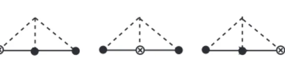
6. The impurity-induced spin-orbit coupling: skew scattering

In this section we discuss skew scattering by considering the diagrams of Fig. 3. To understand the meaning of these diagrams, recall that in general, in the presence of SOC, the scattering amplitude reads

S=A+ ˆp×pˆ⁰·σB, (117) where ˆpand ˆp⁰ are unit vectors in the direction of the momentum before and after the scattering event. To lowest order in perturbation theory or Born approximation one hasA=v0andB=−i(λ²₀p²_F/4)v0and one recov- ers Eq. (92). By considering the scattering probability proportional to|S|², one obtains three contributions given by|A|²,|B|²and 2Re(AB^∗)ˆp×pˆ⁰·σ.

Whereas the first two contributions are spin independent and give the total scattering time, the third one represents the so-called skew scattering term according to which electrons with opposite spin are scattered in opposite directions. Clearly, since Aand B are out of phase, there is no skew scat- tering effect to the order of the Born approximation. For it to appear to first order in the spin-orbit coupling constant λ²₀, A has to be evaluated

Fig. 3. Third order inv0and first order inλ²₀diagrams. The skew scattering contribu- tion arises from the first and last diagram.

beyond the Born approximation. The scattering problem can be cast in terms of the Lippman-Schwinger equation

ψ(x) =e^ik·x+ Z

dx⁰ G(x−x⁰)V(x⁰)ψ(x⁰), (118) where G(x) is the retarded Green function at fixed energy. From (118) we get

ψ⁽¹⁾ =v₀G(x), A⁽¹⁾=v₀; ψ⁽²⁾ =v²₀G(0)G(x), A⁽²⁾=v₀²G(0). (119) Notice that only the imaginary part of A⁽²⁾ is needed. By recalling that Im G(0) =−πN0, the spin-orbit independent scattering amplitudeA up to second order inv₀reads

A=v₀(1−iπN0v₀). (120) The skew scattering contribution will then follow by inserting the modi- fied scattering amplitude (120) into the collision integral of the Boltzmann equation. The same result can, of course, be obtained in quantum field theory using the Green function technique. The latter becomes necessary when one wants to consider skew scattering in the presence of Rashba spin- orbit interaction. To this end one has to consider the electron self-energy at least to third order in the scattering potentialv0. The diagrams of Fig. 3 yield

Σˇ^SSa =−iλ²₀ 4

X

p₁,p₂,p₃,p₄

hVp⁰−p₁Gˇp₁,p₂Vp₂−p₃Gˇp₃,p₄Vp₄−p⁰⁰p4×p⁰⁰·σi Σˇ^SSb =−iλ²₀

4

X

p1,p2,p3,p4

hVp⁰−p₁Gˇp₁,p₂Vp₂−p₃p2×p3·σGˇp₃,p₄Vp₄−p⁰⁰i Σˇ^SSc =−iλ²₀

4

X

p1,p2,p3,p4

hVp⁰−p₁p⁰×p1·σGˇp₁,p₂Vp₂−p₃Gˇp₃,p₄Vp₄−p⁰⁰i. By requiring the existence of third moments of the random potential hV(q1)V(q2)V(q3)i=n_iv³₀δ(q1+q2+q3), we perform the impurity average