Full-counting statistics of time-dependent conductors
M´onica Benito,1Michael Niklas,2and Sigmund Kohler1
1Instituto de Ciencia de Materiales de Madrid, CSIC, 28049 Madrid, Spain
2Institut f¨ur Theoretische Physik, Universit¨at Regensburg, 93040 Regensburg, Germany (Received 29 August 2016; revised manuscript received 27 October 2016; published 21 November 2016) We develop a scheme for the computation of the full-counting statistics of transport described by Markovian master equations with an arbitrary time dependence. It is based on a hierarchy of generalized density operators, where the trace of each operator yields one cumulant. This direct relation offers a better numerical efficiency than the equivalent number-resolved master equation. The proposed method is particularly useful for conductors with an elaborate time dependence stemming, e.g., from pulses or combinations of slow and fast parameter switching.
As a test bench for the evaluation of the numerical stability, we consider time-independent problems for which the full-counting statistics can be computed by other means. As applications, we study cumulants of higher order for two time-dependent transport problems of recent interest, namely steady-state coherent transfer by adiabatic passage (CTAP) and Landau-Zener-St¨uckelberg-Majorana (LZSM) interference in an open double quantum dot.
DOI:10.1103/PhysRevB.94.195433
I. INTRODUCTION
Current fluctuations, while typically undesirable in techni- cal applications, can be useful for understanding quantum- mechanical transport processes [1]. For instance, an open transport channel with transmission close to unity leads to sub-Poissonian noise, while super-Poissonian noise may hint on electron bunching [2], the size of the charge carriers [3], or bistabilities [4–6]. External driving fields enable the control of the noise level via the driving amplitude and frequency [7].
Particular examples of such driven conductors with low current noise are pumps that transport a fixed charge per cycle [8–11].
Moreover, noise measurements may provide evidence for the correct operation of protocols that induce a steady-state version [12] of coherent transport by adiabatic passage [13–15].
Current fluctuations can be characterized by the low- frequency limit of the current correlation function which corresponds to the variance of the transported charge [16].
This allows one to introduce the Fano factor as a dimensionless measure for the noise level using the Poisson process as reference [2]. Going beyond the variance, one may consider the full-counting statistics of the transported electrons [2,4,17–20]
or the related waiting-time distribution of consecutive transport events [21].
For master equation descriptions of time-independent transport, the calculation of the full-counting statistics can be formulated as a non-Hermitian eigenvalue problem with a subsequent computation of derivatives with respect to a counting variable [19]. For systems with very few degrees of freedom, this may provide all cumulants analytically [4,19]. For a numerical treatment, however, one likes to avoid the computation of higher-order derivatives, which can be achieved by an iterative scheme based on Rayleigh- Schr¨odinger perturbation theory [22,23].
These eigenvalue based methods are generally not applica- ble for conductors with an arbitrarytime dependence, so that one has to seek alternatives. One option is a number-resolved master equation in which the number of transported electrons is introduced as an additional degree of freedom [24,25].
However, the distribution of this number may be rather broad and, thus, the computational effort may become tremendous.
A more efficient approach is based on a density-operator-like object that contains information about the second moment of the transported charge [26]. A numerical solution of the corresponding equations of motion provides the current and its variance with moderate numerical effort. With the present work, we extend this idea and derive a propagation method for computing current cumulants up to a given order. Moreover, we show that in the time-independent limit, our method is equivalent to the iteration scheme of Refs. [22,23] and, thus, represents a generalization of these works.
Our paper is structured as follows. In Sec.II, we introduce a master equation description of the full-counting statistics and derive our iteration scheme. In Sec.III, we explore the numerical stability of our method for two time-independent test cases and finally in Sec.IVstudy cumulants of higher order for two driven models of recent interest, namely steady-state coherent transfer by adiabatic passage (CTAP) and Landau- Zener-St¨uckelberg-Majorana (LZSM) interference.
II. GENERALIZED MASTER EQUATION
We consider transport problems that can be captured by a master equation of the form (in units with=1)
˙
ρ= −i[H(t),ρ]+
L(t)ρ≡L(t)ρ, (1) whereH(t) accounts for the coherent quantum dynamics of a central conductor such as a quantum dot array driven by time-dependent gate voltages. The conductor is coupled to two or more electron reservoirs that allow for incoherent electron tunneling from and to the reservoirs. These processes are described by the generally also time-dependent superoperators Lwhich contain the forward and backward current superop- eratorsJ+ andJ−, respectively. For a specific example of these superoperators, see Sec.III.
A. Counting variable
The electron transport can be considered as a stochastic process with the random variable N, the net number of electrons transported to lead, or, equivalently, the electron
number in that lead (to achieve a compact notation, we henceforth suppress the lead indexand the time argument). Its statistical properties can be captured by the moment generating function
Z(χ)= eiχ N =∞
k=0
(iχ)k
k! μk, (2) with the moments μk= Nk =(∂/∂iχ)kZ|χ=0, while their irreducible parts, the cumulantsκk, are generated from lnZ(χ) [27]. For Markovian time-independent transport problems, the cumulants eventually grow linearly in time [19] which motivates the definition of thecurrent cumulantsas the time derivativesck=κ˙k, which are our main quantities of interest.
Their generating function reads φ(χ)= d
dtlnZ(χ)≡ ∞ k=1
(iχ)k
k! ck, (3) which impliesck=(∂/∂iχ)kφ|χ=0.
While the master equation (1) contains the full information about the central conductor, the leads’ degrees of freedom have been traced out in the course of its derivation. To nevertheless keep track of the electron number in lead, one multiplies the full density operator by a counting factoreiχ N for the lead electrons to obtain the generalized density operator R(χ). While its trace is the moment generating function, Z(χ)=trR(χ), the operator R(χ) obeys the generalized master equation [19]
R(χ)˙ =[L+J(χ)]R(χ). (4) The additional term
J(χ)=(eiχ−1)J++(e−iχ−1)J− (5) is composed of the forward and the backward current operators J±mentioned above.
B. Hierarchy of master equations
The generalized master equation (4) together with the generating functions (2) and (3) in principle already provides the current cumulantsck; see Sec.II D. The direct numerical evaluation of these expressions, however, is hindered by two obstacles. First, the numerical computation of derivatives becomes increasingly difficult with the order. Second, the relation between cumulants and moments is known only implicitly via the Taylor series forZ(χ) andφ(χ). Therefore we have to bring the generalized master equation to a form that is more suitable for extracting information about theck.
We start by writing the current cumulant generating func- tion in terms of the generalized density operatorR(χ). From φ=d(lnZ)/dtandZ=trR(χ) together with the generalized master equation (4) follows straightforwardly
φ(χ)= 1
Z(χ)trJ(χ)R(χ)=trJ(χ)X(χ) (6) (notice that trL. . .=0) with the auxiliary operator
X(χ)= 1
Z(χ)R(χ). (7)
Moreover, we find the equation of motion
X(χ˙ )=LX(χ)+[J(χ)−φ(χ)]X(χ). (8) We continue by substituting the dependence on the continuous counting variable χ by the Taylor coefficients Xk and Jk
which we define via the seriesX(χ)=∞
k=0(iχ)kXk/k! and J(χ)=∞
k=1(iχ)kJk/k!. Notice that J(0)=0 such that J0=0 while fork >0, Jk=J++(−1)kJ−. Finally, we obtain from Eqs. (3) and (8) the hierarchy of equations
ck=
k−1
k=0
k k
trJk−kXk, (9) X˙k=LXk+
k−1
k=0
k k
(Jk−k−ck−k)Xk. (10) It constitutes the central formal achievement of this paper and forms the basis of the numerical results presented below.
Two features are worth being emphasized. First, in the limitχ→0,X(χ) becomes the reduced density operator, i.e., for k=0, Eq. (10) is identical to the master equation (1).
Second, as an important consequence ofJ0=0 andc0=0, the summations on the right-hand side of these equations terminate atk=k−1, which implies thatXkandckdepend only on terms of lower order. This enables the truncation at arbitrary order and, thus, the iterative computation of the current cumulants.
The numerical effort of our scheme can be estimated as follows. Let us assume that (if necessary after a full or a partial [28] rotating-wave approximation) the Liouvillian L can be written as ad×d matrix and that its smallest decay rate is γmin. Then to compute the first kmax cumulants, we have to propagatekmaxdscalar equations for a timeτ ≈3/γmin, where one is typically interested in the firstkmax=5–10 cumulants.
To highlight the efficiency of our method, we compare this effort with that of the number-resolved master equation [24,25], for which the density operator is extended by a variable n=0, . . . ,nmax that accounts for the number of transported electrons, truncated atnmax. In the Markovian case, coherences between differentndo not play a role, such that one essentially has to replaceρby thenmax+1 density operators ρ(n), where trρ(n)is the probability thatnelectrons have arrived at lead . During a time τ, on average I τ electrons flow, so that one would have to employ a number-resolved master equation withnmax≈2I τ =6I /γmin, i.e., one has to integrate
∼6I d/γmin scalar equations. This means that wheneverI γmin, our method outperforms this alternative significantly.
This is for example the case when the system infrequently switches between two states with different conductance [4–6].
A further advantage of our method is that it provides direct access to the cumulants, such that the detour via the moments can be avoided.
C. Relation to the iterative scheme for time-independent transport
Equations (9) and (10) resemble the iterative scheme derived in Refs. [22,23] for the cumulants oftime-independent transport problems. Let us therefore establish a connection between both methods. IfLis time independent, the original
master equation possesses a stationary solutionρ∞which for k=0 also solves Eq. (10). Fork >0, we make use of the fact that trX(χ)=1 which implies trXk=δk,0. Consequently, Eq.
(10) possesses also fork >0 a stationary solution. Formally it can be written with the help of the pseudoinverse of the Liouvillian Q/L, where Q=1−ρ∞tr projects to the subspace in which L is regular. Therefore, the condition X˙k =0 together with trXk=δk,0results in
Xk= −Q L
k−1
k=0
k k
(Jk−k−ck−k)Xk, (11) whileX0=ρ∞. Equations (9) and (11) represent the Marko- vian limit of the known iteration scheme for the time- independent case [22,23].
D. Hierarchy of equations for the moments
While the virtue of our scheme is the direct access to the current cumulants, it is worthwhile to compare it with the corresponding iteration for the time-dependent moments derived in Refs. [29,30]. It can be obtained from the Taylor expansions ofZ(χ)=trR(χ) and of the generalized master equation (4) which read
μk= trRk, (12) R˙k=LRk+
k−1
k=0
k k
Jk−kRk, (13) respectively. These equations appear somewhat simpler than the corresponding expressions for the cumulants. However, the subsequent computation of the current cumulants is cumbersome. It can be achieved by the recurrence relation
ck=μ˙k−
k−1
k=1
k−1 k−1
ckμ˙k−k, (14) which follows straightforwardly from Eqs. (2) and (3). Notice that in contrast to Refs. [29,30], we do not consider number cumulants, but current cumulants. Therefore one first has to compute the time derivatives of the moments,
˙
μk =tr ˙Rk=
k−1
k=0
k k
trJk−kRk. (15) The computation of the ck from Eqs. (12)–(15) may be numerically challenging, in particular when, e.g., for strong bunching the cumulants grow rapidly with their order. Then Eq. (14) includes small differences of large numbers, which typically are sensitive to rounding errors.
III. TIME-INDEPENDENT MODELS AS TEST CASES Before addressing time-dependent transport problems, let us start with two time-independent systems which can be solved either analytically or with the iteration scheme of Ref.
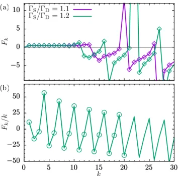
[22]. This allows us to draw conclusions about the numerical stability of our method. To this end, we consider the cumulant ratio
Fk=ck+1/ck, (16)
whereF1is the Fano factor.
Despite the general validity of our formalism, in all applications, we consider an array of n quantum dots with the first dot coupled to an electron sourceS, while the last site is coupled to a drainD. Then the dot-lead tunnelings can be written asLdot-lead=SD(c†1)+DD(cn) with the Lindblad formD(x)ρ=xρx†−12x†xρ−12ρx†x and the tunnel rates S/D. We evaluate the current at the source,=S, such that the forward current operator becomesJS+ρ=Sc1†ρc1, while the backward current operatorJS−vanishes.
1. Single-electron transistor
One of the simplest transport setups is the single-electron transistor which consists of a resonant level between two strongly biased leads. It can be occupied by at most one electron so that the Liouvillian and the forward current operator read
L=
−S D S −D
, J+=
0 0 S 0
, (17) respectively. For the symmetric case,S=D≡, the cumu- lants of the single-electron transistor are known analytically as ck =2−k [19], which makes this system an ideal test case. Consequently, all cumulant ratiosFk=1/2 are identical to the Fano factor. For anyS=D, the cumulants cannot be written in a closed form, but exhibit a generic behavior:
While cumulants of low order reflect the nature of the transport process, high-order cumulants oscillate in a universal manner [31]. Therefore the symmetric case with its constantFk=1/2 is rather special and should be sensitive to numerical errors.
By solving Eqs. (9) and (10) numerically, we have found that forS=D≡, the first30 cumulant ratios agree with the analytical prediction with a precision1% (not shown).
For slight asymmetries, we compare in Fig.1(a)our results with those obtained by the traditional iteration scheme. Both agree rather well also for orders at which the cumulants exhibit universal oscillations.
2. Triple quantum dot in a ring configuration
As a further test case, we consider a ring of three quantum dots, where dots 1 and 3 are coupled to source and drain, respectively. Since in such a ring, the electrons may be transported by direct tunneling from the first to the last dot or via dot 2, the conductance is governed by interference [32,33]
and may suffer from decoherence [34]. Here we consider a gate voltage that shifts the on-site energy of dot 2 bysuch that the corresponding single-particle Hamiltonian reads
H=
⎛
⎝0
0
⎞
⎠. (18)
For strong detuning,, the path via dot 2 has the effective tunnel matrix element2/. Thus in the limit of strong Coulomb repulsion, the situation is that of a slow and a fast channel which block one another [35]. This typically leads to bunching visible in a super-Poissonian Fano factor [4]. The triple quantum dot ring combines several difficulties such as
−5 0 5 10
−50
−25 0 25 50
0 5 10 15 20 25 30
Fk
ΓS/ΓD= 1.1 ΓS/ΓD= 1.2
−5 0 5 10
Fk/k
k
−50
−25 0 25 50
0 5 10 15 20 25 30
FIG. 1. Cumulant ratiosFk=ck+1/ckfor time-independent test cases. The symbols are obtained with our propagation method, while the lines interpolate the results of the iteration scheme based on Eq. (11). (a) Asymmetric single-electron transistor for large bias and various dot-lead rates S/D. (b) Triple quantum dot in ring configuration with S=D=0.1, where dot 2 is detuned by =10. For graphical reasons, we plotFk/k.
different time scales, quantum interference, and cumulants that grow exponentially with their index [35]. The corresponding stiff differential equations represent challenging test cases for propagation methods.
In Fig. 1(b)we again compare the results of our method with those of the iteration of Eq. (11). As for the single electron transistor, we find that for the first 20 cumulants, the results of both methods are practically indistinguishable.
In the present case, calculations for more than roughly 15 cumulants require a rather high numerical precision and, thus, are time consuming. Nevertheless, we can conclude that for the experimentally relevant orders, our scheme is still efficient and numerically stable.
IV. APPLICATIONS
To demonstrate the practical use of our time-dependent iteration scheme, we apply it to two physical situations that have been studied recently, i.e., we generalize previous calculations of the current or the Fano factor to cumulants of higher order.
A. Steady-state coherent transfer by adiabatic passage Let us consider a triple quantum dot in a linear arrangement described by the single-particle Hamiltonian
H(t)=
⎛
⎝ 0 12(t) 0 12(t) 0 23(t)
0 23(t) 0
⎞
⎠. (19)
FIG. 2. (a) Pulsed tunnel matrix elements defined in Eq. (20) which lead to an adiabatic passage of electrons from dot 1 to dot 3.
Each pulse has a widthσ =T /16. The delay within a double pulse is t=T /8, while the time between the pairs is T =40/ max. (b) Corresponding time evolution of the current cumulantsck,k= 1, . . . ,4, for the dot-lead ratesS=D=0.05max[37].
If the tunnel couplingsij are switched adiabatically slowly, the system follows the adiabatic eigenstate∝(23,0,−12)T. In this way, it is possible to transfer an electron from the first dot to the last dot without populating the middle dot [13], an effect known as CTAP. This nonlocal version of an optical Lambda transition [36] has also been predicted for atoms in multistable traps [14,15].
Experimental evidence of the direct tunneling from the first to the last dot is hindered by the backaction of a population measurement, which creates decoherence [38] and, thus, may induce the effect that one wishes to demonstrate. To circumvent this problem, it has been suggested [12] to contact the triple quantum dot to an electron source and drain and to employ the sequence of double Gauss pulses
12/23(t)= ∞ n=0
maxexp
−(t∓t /2−nT)2 2σ2
(20) with widthσ, delayt, and repetition timeT, as is sketched in Fig.2(a). Notice the so-called counterintuitive order of the pulses in which the tunnel matrix element23is active before 12. In the ideal case, this sequence will lead to the transport of one electron per double pulse and, thus, induce a current with a low Fano factor which may serve as experimental verification of CTAP.
While in Ref. [12] only the second current cumulant has been considered, we here focus on cumulants of higher order. We again assume that Coulomb repulsion inhibits the occupation with more than one electron. Then we have to add the empty state to the Hamiltonian (19), while the dissipative parts of the Liouville equation and the current operator remain the same as in the last section.
Figure2(b)shows the time evolution of the first four current cumulants. After a transient stage of roughly ten periods, the dynamics assumes its long-time limit, from which we compute
FIG. 3. Time-averaged population of the central dot for steady- state CTAP as a function of the driving periodT together with the time-averaged cumulants ¯ckfork=2,3,4. All other parameters are as in Fig.2.
the steady-state values of the cumulants as the average over the driving period. The time evolution illustrates that generally the duration of the transient stage increases with the cumulant order.
The central issue of verifying CTAP via noise measure- ments is the correlation between the Fano factor and the population of the middle dot as a function of the driving period T. By contrast, the average current correlates only weakly with the population and cannot serve as indicator [12].
Notice that a nontrivial value for the correlation coefficient requires a nonmonotonic variation of both curves, which indeed is the case. Going beyond this, we plot in Fig. 3 the corresponding cumulants of higher order averaged over one driving period in the long-time limit. We find that the third cumulant also correlates with the occupation, while for the fourth cumulant only the absolute value behaves in this way. Interestingly enough, the profile of the time- averaged cumulants ¯c3 and ¯c4 is even sharper than that of the zero-frequency noise ¯c2considered in Ref. [12]. Thus, the measurement of further cumulants will strengthen the evidence for the correct operation of a steady-state CTAP protocol.
B. Landau-Zener interference
A paradigmatic example for time-dependent quantum mechanics is a two-level system with the single-particle Hamiltonian
H(t)=1 2
(t) −(t)
, (21)
the tunnel matrix element, and the time-dependent bias
(t)=0+Acos(t). (22)
For driving amplitudesA0, the eigenenergies of H(t) as a function of time form avoided crossings. At these crossings, an electron may perform Landau-Zener transitions, such that repeated sweeps lead to the so-called LZSM interference. In a closed system, this is visible in a characteristic pattern of the population as a function of the detuning0and the amplitude A[39]. Having been measured originally for the population of superconducting qubits [40,41], such patterns have been found also for the current in a biased open double quantum dot
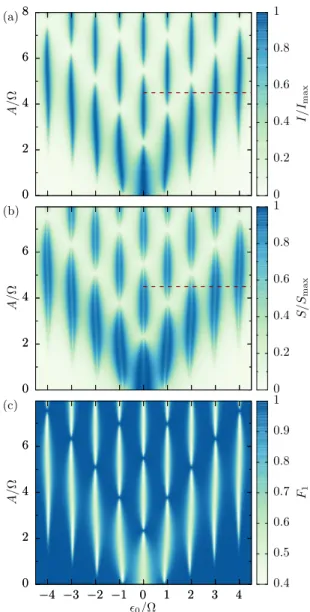
FIG. 4. Average currentI≡c¯1 (a), zero-frequency noise S≡ c¯2(b), and Fano factorF1≡c¯2/c¯1 (c) for a strongly biased driven double quantum dot as a function of the detuning0and the driving amplitudeA. The driving frequency and the dot-lead tunnel rates are =2andS=D=0.15, respectively. The dashed horizontal lines mark the amplitude considered in Fig.5.
[42,43]. For deeper understanding, we extend previous results for the average current to a study of current cumulants.
Figure4(a)shows the LZSM interference pattern for the time-averaged current, i.e., the first cumulant ¯c1. It exhibits the typical structure found in the high-frequency limit, namely Lorentzian resonance peaks which are modulated along theA axis roughly by the squares of Bessel functions [43]. For the second cumulant [Fig.4(b)], the corresponding peaks split into double peaks whose local minima coincide with the current maxima. As a consequence, the corresponding Fano factor [Fig.4(c)] assumes clearly sub-Poissonian values ofF1≈1/2, while off the resonance, the Fano factor indicates Poissonian transport.
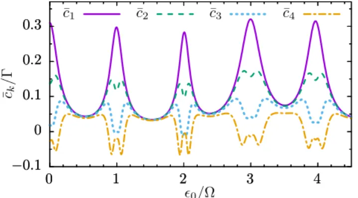
For a closer and more quantitative investigation, we depict in Fig.5the first four cumulants as a function of the detuning 0 for constant driving amplitude. On the one hand, this
FIG. 5. First four cumulants ¯ck for the LZSM interference patterns for the driving amplitude A=4.5 marked in Fig. 4(a) by a horizontal line.
highlights the double peak structure of ¯c2 and indicates that at the edge of the current peaks ¯c2 ≈c¯1which corresponds to the PoissonianF1≈1. The third and fourth cumulants possess a similar double peak structure, where the magnitude of the
¯
ck diminishes with the order k. This affirms the low-noise properties of resonantly driven transport in coupled quantum dots [44].
V. CONCLUSIONS
We have developed a method for the iterative computation of current cumulants for conductors described by time- dependent Markovian master equations. For such transport problems the only generic way to obtain a solution is a numerical propagation while generally eigenvalue-based methods are not applicable. Our scheme is based on a hierarchy of density-operator-like objects truncated according to the desired number of cumulants. The cumulants follow in a direct manner by taking the trace. As compared to the propagation of a number-resolved density matrix, our scheme possesses two advantages. First, it generally gets along with a significantly smaller set of equations. Second, there is no need to compute the cumulants from the moments, a numerically critical task that may involve computing small differences of much larger numbers.
While our aim was the development of a tool for conductors with an arbitrary time dependence, possible applications of our method extend beyond that scope. For example, it may be useful also for obtaining the transients of the counting statistics of time-independent conductors such as those studied in Refs.
[31,45,46]. Moreover, it may be applied to non-Markovian effects that can be captured by time-local master equations with time-dependent coefficients [47]. Finally, for periodic driving, our master equation hierarchy may serve as a starting point for a Floquet treatment of the full-counting statistics. This would extend the approach for the second cumulant derived from a precursor of the present method [48].
As a test bench, we have employed two time-independent master equations which can be solved also with previously known eigenvalue-based methods. It turned out that our scheme provides reliable results for roughly the first 15 cumulants even for challenging test cases. For less demanding situations, computing more than 30 cumulants is feasible.
Thus, we reach orders way beyond the present experimental needs.
We have applied our scheme to two time-dependent systems of recent interest. For steady-state CTAP, we have found that not only the second cumulant, but also higher ones correlate with the population of the middle dot. Therefore they may provide additional evidence for the correct operation of a CTAP protocol. A similar conclusion can be drawn for Landau-Zener interference patterns of the current in open double quantum dots. The higher-order cumulants substantiate the conclusions drawn from studies of the Fano factor on the low noise properties of resonantly driven transport.
In this spirit, our approach enables the computation of the current noise for time-dependent transport beyond the second cumulant with a moderate effort. This may provide additional insight to the underlying mechanisms and a deeper understand- ing of the electron dynamics controlled by arbitrarily shaped pulses.
ACKNOWLEDGMENTS
This work was supported by the Spanish Ministry of Economy and Competitiveness via Grant No. MAT2014- 58241-P and the FPI program and by the DFG via SFB 689.
[1] C. Beenakker and C. Sch¨onenberger, Phys. Today 56(5), 37 (2003).
[2] Y. M. Blanter and M. B¨uttiker,Phys. Rep.336,1(2000).
[3] X. Jehl, M. Sanquer, R. Calemczuk, and D. Mailly, Nature (London)405,50(2000).
[4] W. Belzig,Phys. Rev. B71,161301(R)(2005).
[5] J. Koch and F. von Oppen,Phys. Rev. Lett.94,206804(2005).
[6] N. Lambert, F. Nori, and C. Flindt,Phys. Rev. Lett.115,216803 (2015).
[7] S. Camalet, J. Lehmann, S. Kohler, and P. H¨anggi,Phys. Rev.
Lett.90,210602(2003).
[8] L. Fricke, M. Wulf, B. Kaestner, V. Kashcheyevs, J. Timoshenko, P. Nazarov, F. Hohls, P. Mirovsky, B. Mackrodt, R. Dolata, T.
Weimann, K. Pierz, and H. W. Schumacher,Phys. Rev. Lett.
110,126803(2013).
[9] B. Kaestner and V. Kashcheyevs,Rep. Prog. Phys.78,103901 (2015).
[10] A. Croy and U. Saalmann,Phys. Rev. B93,165428(2016).
[11] M. Kataoka, N. Johnson, C. Emary, P. See, J. P. Griffiths, G. A.
C. Jones, I. Farrer, D. A. Ritchie, M. Pepper, and T. J. B. M.
Janssen,Phys. Rev. Lett.116,126803(2016).
[12] J. Huneke, G. Platero, and S. Kohler, Phys. Rev. Lett. 110, 036802(2013).
[13] A. D. Greentree, J. H. Cole, A. R. Hamilton, and L. C. L.
Hollenberg,Phys. Rev. B70,235317(2004).
[14] K. Eckert, M. Lewenstein, R. Corbal´an, G. Birkl, W. Ertmer, and J. Mompart,Phys. Rev. A70,023606(2004).
[15] R. Menchon-Enrich, A. Benseny, V. Ahufinger, A. D. Greentree, Th. Busch, and J. Mompart,Rep. Prog. Phys.79,074401(2016).
[16] D. K. C. MacDonald,Rep. Prog. Phys.12,56(1949).
[17] M. B¨uttiker,Phys. Rev. B46,12485(1992).
[18] L. S. Levitov and G. B. Lesovik, Pis’ma Zh. Eksp. Teor. Fiz.58, 225 (1993) [JETP Lett.58, 230 (1993)]
[19] D. A. Bagrets and Y. V. Nazarov, Phys. Rev. B67, 085316 (2003).
[20] J. Cerrillo, M. Buser, and T. Brandes,arXiv:1606.05074.
[21] T. Brandes,Ann. Phys. (Leipzig)17,477(2008).
[22] C. Flindt, T. Novotn´y, A. Braggio, M. Sassetti, and A.-P. Jauho, Phys. Rev. Lett.100,150601(2008).
[23] C. Flindt, T. Novotn´y, A. Braggio, and A.-P. Jauho,Phys. Rev.
B82,155407(2010).
[24] S. A. Gurvitz and Ya. S. Prager, Phys. Rev. B 53, 15932 (1996).
[25] B. Kubala, J. Ankerhold, and A. D. Armour,arXiv:1606.02200.
[26] R. S´anchez, S. Kohler, and G. Platero,New J. Phys.10,115013 (2008).
[27] N. G. van Kampen, Stochastic Processes in Physics and Chemistry(North-Holland, Amsterdam, 1992).
[28] D. Darau, G. Begemann, A. Donarini, and M. Grifoni,Phys.
Rev. B79,235404(2009).
[29] D. Kambly, C. Flindt, and M. B¨uttiker,Phys. Rev. B83,075432 (2011).
[30] D. Kambly and C. Flindt,J. Comput. Electron.12,331(2013).
[31] C. Flindt, C. Fricke, F. Hohls, T. Novotn´y, K. Netoˇcn´y, T.
Brandes, and R. J. Haug,Proc. Natl. Acad. Sci. U.S.A.106, 10116(2009).
[32] C. Emary, D. Marcos, R. Aguado, and T. Brandes,Phys. Rev. B 76,161404(2007).
[33] M. Niklas, A. Trottmann, A. Donarini, and M. Grifoni, arXiv:1610.08447.
[34] C. W. Groth, B. Michaelis, and C. W. J. Beenakker,Phys. Rev.
B74,125315(2006).
[35] F. Dom´ınguez, G. Platero, and S. Kohler,Chem. Phys.375,284 (2010).
[36] N. V. Vitanov, T. Halfmann, B. W. Shore, and K. Bergmann, Annu. Rev. Phys. Chem.52,763(2001).
[37] Notice that in the figures and captions of Ref. [12], all times should be multiplied by a factor 20, while the ratesandγ should be divided by 10.
[38] J. Rech and S. Kehrein,Phys. Rev. Lett.106,136808(2011).
[39] S. N. Shevchenko, S. Ashhab, and F. Nori,Phys. Rep.492,1 (2010).
[40] W. D. Oliver, Y. Yu, J. C. Lee, K. K. Berggren, L. S. Levitov, and T. P. Orlando,Science310,1653(2005).
[41] M. Sillanp¨a¨a, T. Lehtinen, A. Paila, Y. Makhlin, and P. Hakonen, Phys. Rev. Lett.96,187002(2006).
[42] J. Stehlik, Y. Dovzhenko, J. R. Petta, J. R. Johansson, F.
Nori, H. Lu, and A. C. Gossard,Phys. Rev. B86,121303(R) (2012).
[43] F. Forster, G. Petersen, S. Manus, P. H¨anggi, D. Schuh, W.
Wegscheider, S. Kohler, and S. Ludwig,Phys. Rev. Lett.112, 116803(2014).
[44] M. Strass, P. H¨anggi, and S. Kohler,Phys. Rev. Lett.95,130601 (2005).
[45] D. Marcos, C. Emary, T. Brandes, and R. Aguado,Phys. Rev. B 83,125426(2011).
[46] P. Stegmann and J. K¨onig,Phys. Rev. B94,125433(2016).
[47] H. P. Breuer, B. Kappler, and F. Petruccione,Ann. Phys.291, 36(2001).
[48] F. J. Kaiser and S. Kohler,Ann. Phys. (Leipzig)16,702(2007).