Trans-Atlantic Equatorial cruise I Cruise No. M158
September 19 – October 26, 2019 Walvis Bay (Namibia) – Recife (Brazil)
P. Brandt, C. Begler, P. Coelho, R. Czeschel, P. Dennert, A. Fernandez Carrera, A.
Filella, S. Gindorf, M. Gómez-Letona, A. C. Hans, F. Heukamp, R. Kiko, B. Kisjeloff, R. A. Imbol Koungue, I. Kriest, W. Martens, A. Prigent, B. Ramcharitar, A. N.
Sarmiento Lezcano, S. Schmidtko, J. Schrandt, J. Sherman, M. Stelzner, T.
Stoeven, A. Subramaniam, F. P. Tuchen Prof. Dr. Peter Brandt
GEOMAR Helmholtz-Zentrum für Ozeanforschung Kiel
2019
Table of Content
1 Summary ... 4
2 Participants ... 5
2.1 Principal Investigators ... 5
2.2 Scientific Party ... 5
2.3 Participating Institutions ... 5
3 Research Program... 6
3.1 Description of the Work Area ... 6
3.2 Aims of the Cruise ... 6
3.3 Agenda of the Cruise ... 7
4 Narrative of the Cruise... 7
5 Preliminary Results ... 9
5.1 Hydrographic observations ... 9
5.1.1 CTD system, oxygen measurements, and calibration ... 9
5.1.2 Conductivity measurements ... 11
5.1.3. Oxygen Winkler measurements ... 12
5.1.4 Thermosalinograph ... 12
5.2 Current observations ... 12
5.2.1 Vessel mounted ADCP ... 12
5.2.2 Lowered ADCP ... 13
5.3 Drifter and floats ... 14
5.4 Mooring operations ... 14
5.4.1 Instrument performance ... 15
5.4.2 Calibration of moored instruments ... 16
5.5 Shipboard microstructure measurements ... 16
5.6 X-band Radar ... 17
5.7 Biochemical measurements ... 17
5.7.1 Tracermeasurements ... 17
5.7.2 Underwater Vision Profiler ... 19
5.7.3 Underwater Microscope ... 20
5.7.4 Acoustic Zooplankton and Fish Profiler, Mulitnet ... 20
5.7.5 Nutrient measurements ... 21
5.7.6 Biogeochemistry of nitrous oxide (N2O) ... 22
5.7.7 N2 Fixation, Primary productivity ... 22
5.7.8 HPLC, flow cytometry, photophysiology ... 22
5.7.9 Organic matter ... 23
5.7.10 Prokaryotes ... 25
5.8 Hydrosweep, topography ... 26
6 Ship´s Meteorological Station ... 26
7 Station Lists M158 ... 28
7.1 Station list ... 28
7.2 CTD Station list ... 35
7.3 Drifter and float deployments ... 38
7.3.1 SVP buoy deployments... 38
7.3.2 CARTHE drifter deployments ... 39
7.3.3 Argo float deployments ... 39
7.4 List of mooring deployments and recoveries ... 40
7.4.1 Mooring Recoveries ... 40
7.4.2 Mooring Deployments ... 41
7.5 Microstructure station list ... 42
7.6 CPICS deployment list ... 43
7.7 Biogeochemical sampling station list ... 44
8 Data and Sample Storage and Availability ... 46
9 Acknowledgements ... 47
10 References ... 47
11 Appendix – List of Abbreviations ... 47
1 Summary
The Transatlantic Equatorial Cruise I (TRATLEQ I) was an interdisciplinary cruise focusing on upwelling in the tropical Atlantic, its physical forcing, its importance for biological production and plankton communities, associated chemical cycles, as well as on the current system setting the background conditions for the downward carbon export. This cruise represents the first physical, chemical, biogeochemical and biological measurement program covering a whole equatorial section from the eastern to the western boundary and from the surface to the bottom. TRATLEQ I is a contribution to the GEOMAR research program OCEANS, to the EU projects TRIATLAS, the „Make Our Planet Great Again“ project by R. Kiko and to the BMBF cooperative project BANINO in the frame of the BMBF SPACES program.
Beside the equatorial Atlantic, another study area was the coastal upwelling off Angola, where the same techniques were applied to better understand the functioning of this tropical upwelling system. A particular focus is on the export flux of carbon to mesopelagic and bathypelagic depths associated with particle flux and diel vertical zooplankton migration. Physical ocean dynamics were studied by full-ocean-depth current measurements and tracer distributions allowing to quantify ventilation and water mass exchange between the western and the eastern boundary. The measurement program also included the service of long-term moorings at the equator at 23°W and off Angola at 11°S.
Zusammenfassung
Die „Transatlantische Äquatoriale Forschungsfahrt I“ (TRATLEQ I) konzentrierte sich mit interdisziplinären Arbeiten auf ein besseres Verständnis von ozeanischem Auftrieb, seinem physikalischen Antrieb, seiner Bedeutung für die biologische Produktivität und die Planktongemeinschaften, den mit ihm verbundenen chemischen Umsatzraten, sowie dem Strömungssystem, das die Hintergrundbedingungen für den Kohlenstoffexport in die Tiefe setzt.
TRATLEQ I war die erste Forschungsfahrt mit physikalischen, chemischen, biogeochemischen, und biologischen Messungen, die den gesamten atlantischen Äquator vom östlichen bis zum westlichen Rand und von der Oberfläche bis zum Meeresboden erfasst hat. Neben dem äquatorialen Atlantik wurde auch das Küstenauftriebsgebiet vor Angola untersucht. TRATLEQ I trägt zum GEOMAR Forschungsprogramm OCEANS, zum EU Projekt TRIATLAS, zum „Make Our Planet Great Again“ Projekt von R. Kiko und zum BMBF Verbundprojekt BANINO im Rahmen des BMBF SPACES Programms bei.
Ein besonderer Schwerpunkt ist die Untersuchung des Kohlenstoffexports in größere Tiefen aufgrund von Teilchentransport und täglicher vertikaler Zooplanktonwanderung. Die physikalische Ozeandynamik wurde insbesondere mit Strömungs- und Tracermessungen studiert und soll eine Quantifizierung der Ventilation und des Wassermassenaustauschs zwischen westlichem und östlichem Rand erlauben. Das Messprogramm beinhaltete auch den Tausch von Langzeitverankerungen am Äquator bei 23°W und vor Angola bei 11°S.
2 Participants
2.1 Principal Investigators
Name Institution
Brandt, Peter, Prof. GEOMAR
Kiko, Rainer, Dr. GEOMAR
2.2 Scientific Party
No. Name Discipline Institution
1 Brandt, Peter, Prof. PO, Chief Scientist GEOMAR
2 Schmidtko, Sunke, Dr. PO, CTD GEOMAR
3 Czeschel, Rena, Dr. PO, vmADCP, LADCP, CTD GEOMAR 4 Imbol Koungue, Rodrigue
Anicet, Dr.
PO, RapidCast, CTD, radar GEOMAR 5 Tuchen, Franz Philip PO, Microstructure, CTD,moored profiler GEOMAR
6 Begler, Christian PO, Moorings, logistics GEOMAR
7 Kisjeloff, Boris PO, Moorings/O2 logger, salinometer GEOMAR
8 Martens, Wiebke PO, CTD technique GEOMAR
9 Prigent, Arthur PO, CTD, Argo, SVP, CARTHE GEOMAR 10 Dennert, Peter PO, CTD, salinometer, microstructure GEOMAR
11 Heukamp, Finn PO, CTD, microstructure GEOMAR
12 Hans, Anna Christina PO, CTD, Argo, SVP, CARTHE GEOMAR
13 Coelho, Paulo PO, CTD watch, ADCP INIPM
14 Stoeven, Tim, Dr. CO, Tracer GEOMAR
15 Schrandt, Julia CO, Tracer GEOMAR
16 Kriest, Iris, Dr CO, Tracer GEOMAR
17 Gindorf, Sonja CO, N2O GEOMAR
18 Subramaniam, Ajit, Prof. BO, Biooptics, phytoplankton, LDEO 19 Ramcharitar, Benjamin BO, Primary production LDEO 20 Sherman, Jonathan BO, Biooptics, phytoplankton RUTGERS 21 Fernandez Carrera, Ana Dr. BO, Nitrogen fixation, Nutrients UVIGO 22 Kiko, Rainer, Dr. BO, Zooplankton, multinet, UVP, oxygen GEOMAR
23 Gómez-Letona, Markel BO, DOM, cDOM, POC ULPGC
24 Sarmiento L., Airam Nauzet BO, AZFP ULPGC
25 Filella, Alba BO, DOM, cDOM, POC GEOMAR
26 Stelzner, Martin Meteorology DWD
27 Fonseca Figueredo, Adriana Observer Brazilian Navy
PO: Physical Oceanography, CO: Chemical Oceanography, BO: Biological Oceanography
2.3 Participating Institutions
GEOMAR GEOMAR Helmholtz-Zentrum für Ozeanforschung Kiel, Germany DWD Deutscher Wetterdienst, Germany
INIPM Instituto Nacional de Investigação Pesqueira e Marinha, Luanda, Angola LDEO Lamont Doherty Earth Observatory at Columbia University, USA RUTGERS Institute of Marine and Coastal Sciences, Rutgers University, USA ULPGC University of Las Palmas de Gran Canaria, Spain
UVIGO Universidade de Vigo, Spain
3 Research Program
3.1 Description of the Work Area
The research program of TRATLEQ I (Fig. 3.1) covered two main research areas that are 1) the tropical coastal upwelling area off Angola and 2) the equatorial Atlantic. Focus areas were the 11°S section off Angola and the whole equatorial section from 5°E to 44°45’W. Additional measurements were performed underway and at a few CTD stations along the cruise track from Walvis Bay to 11°S and from 11°S to the first station on the equatorial section at 5°E. The work off Namibia and Angola covered the eastern boundary upwelling system. The seasonal upwelling off Angola was at its secondary minimum during the period of the cruise. Due to the refusal of the diplomatic application, no measurements could be performed in the territorial waters of Equatorial Guinea. The equatorial section covered the Atlantic cold tongue that represents the equatorial upwelling system east of 23°W and the western equatorial Atlantic characterized by warmer surface waters and deeper mixed layer depths. The equatorial upwelling was in its mature phase during which maximum carbon export from the upper ocean into the deep was expected.
Fig. 3.1. Bathymetric map with cruise track of R/V METEOR cruise M158 (grey solid line) including locations of CTD/UVP/LADCP/AZFP stations, mooring recoveries and redeployments, microstructure and multinet stations and locations of drifter and float deployments. Territorial waters of different countries are marked with thin black solid lines.
3.2 Aims of the Cruise
TRATLEQ I was an interdisciplinary cruise focusing on upwelling in the tropical Atlantic, its physical forcing, its importance for biological production and plankton communities, associated chemical cycles, as well as on the current system setting the background conditions for the downward carbon export. This cruise represents the first physical, chemical, biogeochemical and biological measurement program covering a whole equatorial section from the eastern to the western boundary and from the surface to the bottom. A general aim of the research cruise was to assess the status of the southeast and equatorial Atlantic marine ecosystem, to identify its physical
drivers and the impact of climate variability and change. A central question was which role does circulation and mixing play for the development of phytoplankton and zooplankton communities and specifically how variable (regionally and seasonally) is the export flux of carbon to mesopelagic and bathypelagic depths associated with particle flux and diel vertical zooplankton migration.
3.3 Agenda of the Cruise
The measurement program of TRATLEQ 1 included the section work along 11°S off Angola and along the equator starting at 5°E off São Tomé and Príncipe and ending at 44°45’W on the Brazilian shelf. Observations along the sections included full-depth station work with the CTD system measuring temperature, salinity, pressure, oxygen, nutrients (NOx), turbidity, fluorescence (i.e. chlorophyll- a and fluorescent dissolved organic matter (fDOM)), current velocity with the lowered acoustic Doppler current profilers (LADCP), particle size classes and plankton composition with an underwater vision profiler 5 (UVP5) and a continuous particle imaging and classification system (CPICS), as well as backscatter measurements with an acoustic zooplankton and fish profiler (AZFP). The CPICS was only operated on the CTD off Angola and then was deployed separately on shallower 110 m casts due to pressure-related problems.
Additional station work was carried out with a microstructure profiler measuring turbulent dissipation rates in the upper 100 m, and an Hydrobios Multinet Midi for the collection of zooplankton samples in the upper 1000 m. Water samples were analyzed for numerous variables including salinity, oxygen, tracer (CFC-12, SF6), nutrients, N2O, and colored dissolved organic matter (cDOM). N2-fixation and primary production rates were determined through incubation of collected seawater. Underway measurements were performed with the two shipboard ADCPs for velocities in the upper 1000 m, the thermosalinograph for near-surface temperature and salinity, and a throughflow system for near-surface fluorescence intensity and phytoplankton physiological state via Fluorescence Induction Relaxation experiment (FIRe) and Picosecond Lifetime Fluorescence (PicoLif) measurements. Depth resolved FIRe measurements were also conducted using water samples from the CTD-Rosette. With regard to the original cruise proposal all proposed work could be performed with some slight deviations that include underway measurements of N2O, CO2, O2 and total gas tension (due to the visa problems of few scientists not able to attend the cruise) and a malfunction of the RapidCast underway CTD system, where planned quasi-continuous measurements along the Namibian and Angolan shelf were replaced by on-station work with CTD and microstructure probe.
4 Narrative of the Cruise
On Thursday, September 19, 2019, R/V METEOR departed from the harbor of Walvis Bay, Namibia at about noon. The small delay was due to some late delivery of scientific equipment.
More importantly, however, was that three members of the scientific team could not join the cruise because of visa issues. Two colleagues, with passports from countries that are not allowed to enter Namibia without a visa, were not able to enter Namibia. Another colleague from Angola (also acting as second observer) did not receive his visa for Brazil in time. Unfortunately, this also means that some measurements, like e.g. various biogeochemical underway measurements, could not be carried out as planned.
Sampling by the underway systems that included sea surface temperature, salinity, fluorescence intensity, upper ocean velocity and X-band radar measurements was started on September 19 at 14:00 UTC. The station work on the Angolan/Namibian shelf began on September 20 with the first CTD and MSS stations. Planned underway measurements of upper ocean temperature and salinity with the RapidCast system could not be performed due to the failure of the communication between the winch and the board unit that could not be fixed during the cruise. Instead, we decided to perform measurements approximately along the 500-m depth contour with the CTD and the MSS on a regular 1° latitude resolution while progressing northward. We arrived at 11°S on September 22 at 14:00 UTC. Along 11°S, we started with CTD and MSS measurements at very high spatial resolution. Since July 2013, we service a long-term mooring located at the continental slope measuring the strength of the southward Angola Current. This mooring had surfaced accidentally in July 2019 and could be recovered by Angolan colleagues from the Regional Centre of the National Fisheries and Aquaculture Inspection Service of Kwanza Sul, Angola. On September 23, Angolan colleagues delivered the recovered mooring to R/V Meteor off the port of Porto Amboím close to our measurement area. The main moored instrument, an upward looking ADCP, was still working properly, thus complementing the long-term velocity time series of the Angola Current. After mooring delivery, we continued with CTD and MSS station work along the 11°S section. At the nominal position of the mooring we did our first station with the multinet aimed at collecting zooplankton samples and characterizing the zooplankton community. Due to the diurnal vertical migration, we tried as much as possible during the cruise to have day and night stations with the multinet capturing diurnal differences in the zooplankton distribution. At the offshore end of the 11°S section, we deployed three Argo floats in deeper waters. The redeployment of the Angola Current mooring started on September 25 at 15:40 and could be finished without problems at 18:00. Additional to the standard tall mooring, we also deployed a pressure inverted echo sounder (PIES) that will be used to measure the variability in the bottom pressure difference between Brazil and Angola thereby delivering the mean geostrophic velocity anomaly across the Atlantic. After finishing the mooring and station work along 11°S, we continued underway measurements along the 500-m depth contour until the last CTD station at 6°27’S close to the border of the EEZ of Angola.
On the way toward the equator, we had to stop with all measurements when entering the EEZ of Equatorial Guinea as we did not receive allowance for measurements by this country.
We arrived at the equator at 5°E in the EEZ of São Tomé and Príncipe on September 28 at 23:00 UTC. Here, we started the main work along the trans-Atlantic equatorial section. Work at 5°E included double CTD stations to fulfill the extended requirements of all groups for water samples, MSS measurements and a multinet station. Here we also released an Argo float and we started a series of surface drifter deployments along the equator. We had two different drifters on board, the standard SVP drifters, which drift with the water at 15 m depth and CARTHE drifters measuring the velocity in the upper meter. Pairs of drifters were deployed every 1° longitude between 10°W and 30°W with some lower resolution toward east and west. The combined drifter data will allow us to assess the vertical shear of the flow field close to the surface.
After a short break due to another passing of the EEZ of Equatorial Guinea, we continued station work on September 29 at 20:00 at 2°E. Along the section, we did CTD and MSS stations every 1° longitude and multinet stations every few degrees. All sensors worked continuously
without problems. After few stations the CPICS camera system developed a leakage but could be repaired and was in the following only used during shallow 110 m casts.
On October 8, we arrived at 18°W, where we deviated from the equatorial section to perform a short meridional section with the shipboard ADCP between 0°45’N/S to identify the latitudinal core location of the Equatorial Undercurrent and equatorial deep jets. On October 11 at 15:00 UTC, we reached the mooring position of the long-term mooring at 23°W. This mooring is operated in cooperation with the French PIRATA project since December 2001. Data of this mooring are used in many publications studying diverse topics such as the equatorial circulation, tropical climate, oxygen distribution and variability, sinking of particles at the equator and downward carbon flux. After having a day-time cast with the multinet, we recovered the mooring without problems. All instruments had worked throughout the mooring period with the moored profiler having a depth range slightly degrading with time. This gives us another excellent dataset to study long-term changes in the equatorial ocean. During the night, we did some CTD, MSS and multinet stations. The deployment of the equatorial mooring began on the next morning at 09:00 UTC and was finished four and a half hours later. We could nicely observe the submergence of the top-element confirming the successful deployment procedure. At the mooring, for the first time, two UVPs were installed to continuously measure particles (100 µm to about 2 cm) at 300 and 800 m depths.
After the mooring work was finished we continued with station work at a resolution of 1°
longitude. When approaching the western boundary starting at 37°W, we decreased the distance between stations to 30’ longitude and close to the continental slope we decreased it further to 5’
longitude to capture the very narrow boundary currents. The last CTD station at the equator at 44°15’W was finished on October 22 at 07:30 UTC. We continued the section along the equator until 44°45’W doing particularly underway velocity measurements to capture also the shallow part of the North Brazil Current. After finishing the equatorial section, we turned back to a south- eastward direction heading toward the final destination, the port of Recife, where we arrived on October 26 at 09:00 UTC.
5 Preliminary Results
5.1 Hydrographic observations
5.1.1 CTD system, oxygen measurements, and calibration (Sunke Schmidtko)
5.1.1.1 CTD-Rosette system
During M158 a total of 102 CTD-profiles and 2281 water samples were collected. The rosette system was installed in a Seabird Rosette System frame for 24 bottles. Most casts were made with 22 bottles installed, except casts made for the calibration of MicroCATs. Depth profiles up to a maximum pressure of 6048 dbar were performed. Deeper profiles were not possible due the maximum depth rating of installed instruments of 6000 m. For the majority of stations, the full water column was sampled. Data acquisition was done using Seabird Seasave software version 7.23.2. Preprocessing was done with SBE Data Processing 7.23.2.
The first CTD profile was collected at instrument test station #1. It was determined that all sensors recorded data with sufficient accuracy and no errors were detected. On the downcast of profile #79, there was a blackout of the CTD pump. The cast was canceled, but water samples were still taken. To analyze the cause of pump failure, conductivity sensors on the CTD were
switched. However, the wrong configuration was loaded in the deck unit for that profile (#80). The raw data files were reprocessed after editing of the configuration xml-files. The conductivity sensors were swapped back for the following profiles and the CTD system worked without problems for the final 41 profiles. The oxygen sensors provided high quality reliable data throughout the cruise. The exact configuration of the CTD system can be found in Table 5.1.
Additionally, two self-recording LADCPs, a self-recording, self-powered UVP5, a self-recording nutrient sensor, a self-recording, self-powered AZFP, and a self-recording, self-powered CPICS were attached to the water sampler. They are described separately in this cruise report.
Processed preliminary CTD data, 5-dbar binned, was sent in near real time to the Coriolis Data Centre in Brest, France, (via email: codata@ifremer.fr) for integration in the databases to be used for operational oceanography applications and the WMO supported GTS/TESAC system.
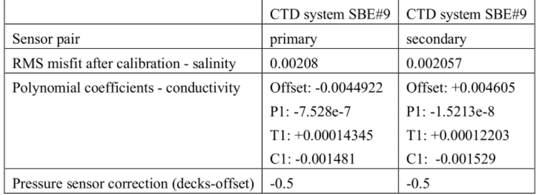
Table 5.1. Summary of CTD system SBE #9 configuration used during M158.
CTD system SBE#9 (all except 80) CTD system SBE#9 (cast 80)
Pressure sensor # 1149 # 1149
T primary # 2463 # 2463
T secondary # 2120 # 2120
C primary # 2443 # 3959
C secondary # 3959 # 2443
O2 primary SBE 43 # 1312 SBE 43 # 1312
O2 secondary SBE 43 # 1739 SBE 43 # 1739
PAR Sensor # 70714 # 70714
Altimeter # 42299 # 42299
WET Labs ECO-AFL/FL # 2294 # 2294
5.1.1.2 CTD-conductivity calibration
Overall 232 calibration points were obtained by sampling for salinity. Salinity samples were taken by the CTD watch in ‘Flensburger’ bottles, which proofed to be ideal for storing salt samples over a long time. The limited amount of bottle cases brought along required the washing and reuse of eight boxes. Reused bottles were used for salt samples from cast 42 onwards. Measurements are described in section 5.1.2. Due to the large number of samples a simple outlier removal method was applied that discharged the largest 33% deviations between CTD and bottle samples prior to calibration. The projection of data taken during the bottle stops of the upcast to the data from the downcast was done by searching within a 30-dbar pressure interval for similar potential temperatures. For the critical loop edit velocity 0.01m/s was used. The final CTD data set is composed from the primary set of sensors for all profiles, though the differences between sensor pairs were marginal. The conductivity calibration of the downcast data was performed using a 1st order linear fit with respect to temperature, pressure and conductivity (Table 5.2).
The calibration results in a salinity RMS-misfit for the downcast of order 0.00258 for the primary and 0.00267 for the secondary sensor. The upcast calibration surpasses these values with a RMS-misfit of 0.00208 psu for the primary and 0.00206 psu for the secondary sensor.
Table 5.2. End of cruise salinity and pressure summary of downcast calibration information for the two CTD systems used during M116.
CTD system SBE#9 CTD system SBE#9
Sensor pair primary secondary
RMS misfit after calibration - salinity 0.00208 0.002057 Polynomial coefficients - conductivity Offset: -0.0044922
P1: -7.528e-7 T1: +0.00014345 C1: -0.001481
Offset: +0.004605 P1: -1.5213e-8 T1: +0.00012203 C1: -0.001529 Pressure sensor correction (decks-offset) -0.5 -0.5
5.1.1.3 Oxygen calibration
The CTD oxygen downcast for CTD systems is calibrated by using the best 66% of the joint data pairs between downcast CTD sensor value and Winkler-titrated oxygen (Section 5.1.3). For the calibration a linear correction polynomial depending on pressure, temperature and the actual oxygen value was fitted (Table 5.3). A total of 403 oxygen data points for CTD system SBE#5 were recorded, which resulted in an RMS-misfit for the downcast of 1.0859 µmol kg-1 for the primary SBE43 and 1.0143 µmol kg-1 for the secondary SBE43. The upcast calibration even surpassed these very good values with a RMS-misfit of 1.0489 µmol kg-1 for the primary SBE43 and 1.0105 µmol kg-1 for the secondary SBE43.
Table 5.3. End of cruise downcast oxygen summary of calibration information for the CTD system SBE#9 used during M158.
Oxygen Sensor #1312 Oxygen Sensor #1739
Sensor pair primary secondary
RMS misfit after calibration - oxygen 1.0859 1.0143 Polynomial coefficients - oxygen Offset: -2.2712
P1: 0.0032034 T1: 0.060801 O1: 0.030105
Offset: -0.68345 P1: 0.0025876 T1: 0.097481 O1: 0.055254
5.1.2 Conductivity measurements
(Boris Kisjeloff, Peter Dennert, Sunke Schmidtko)
In order to calibrate the conductivity sensors of the CTD system, the conductivity of more than 500 water samples was measured using the GEOMAR OPTIMARE Precision Salinometer (OPS) 10. The OPS has been tested for several years both in GEOMAR laboratories and on prior research cruises (see e.g. cruise report of RV Maria S. Merian MSM60). Before measuring the conductivity of the water samples with the OPS, the bottled water samples had to be degassed to remove gas micro-bubbles, which would deteriorate the OPS instrument performance. Degassing was done after warming the sample bottles in a water bath at a temperature of about 40°C. After approximately one hour the bottles were removed from the bath. The Flensburger bottles were opened shortly to release the gas. Afterwards the sample bottles were brought to the salinity lab where their conductivity could be measured after 24 hours of cooling down to the lab temperature.
During the cruise we realized a strong drift in the salinity measurements. Even with enhanced use of substandard and standard waters the measurements were not useful for calibration.
Therefore, we tried to clean the Salinometer with distilled waters. However, further jumps of several thousandth PSU were noticed during the measurements. Therefore, we exchanged the bath of the already broken Salinometer 020 with the Salinometer 010. This led to a functioning Salinometer 020 which allowed for valuable measurements for the calibration of the CTD.
5.1.3. Oxygen Winkler measurements (Rainer Kiko)
Discrete samples from selected depths were analyzed for oxygen at the majority of the stations.
Bubble free samples were taken in 100 ml ground flasks, treated with alkaline sodium iodide and manganese chloride solutions and analyzed within eight hours after fixation using the Winkler method. In short, the precipitated hydroxides were dissolved with 1 ml sulphuric acid and the liberated iodine was then titrated to a light-yellow color using sodium thiosulfate. Thereafter, a zinc starch solution was added and the titration continued until the blue color disappeared. During the entire cruise three 1 l sodium thiosulfate bottles were prepared and used. For each bottle the calibration factor was determined using a WAKO iodate standard (batch no TWJ0275), see Table 5.4. In total 410 niskin bottles from 89 CTD profiles were sampled. The respective measurements were used to calibrate the profiling sensor of the CTD.
Table 5.4. Calibration factors of sodium thiosulfate bottles.
Date Factor
Sep. 21, 2019 - Oct. 02, 2019 1.00181315 Oct. 03, 2019 - Oct. 19, 2019 0.99706067 Oct. 20, 2019 - Oct. 24, 2019 0.99440646
5.1.4 Thermosalinograph
(Anna Cristina Hans, Sunke Schmidtko)
Underway measurements of sea surface temperature (SST) and sea surface salinity (SSS) were continuously done by the ship’s dual thermosalinograph. One inlet is located at the portside (TSG1) while the other thermosalinograph’s inlet is at the starboard side (TSG2). The parallel system worked well and continuously throughout M158. Only data gaps were due to the switch off of scientific measurements in the EEZ of Equatorial Guinea. SSS and SST measured by the TSG system was calibrated with CTD measurements at 5m, with a resulting rms in SST of 0.005
°C and a resulting rms in SSS of <0.01.
5.2 Current observations 5.2.1 Vessel mounted ADCP
(Rena Czeschel, Rodrigue Anicet Imbol Koungue)
Underway-current measurements of the upper ocean were performed continuously throughout the entire cruise (except in the territorial waters of Equatorial Guinea) using two Vessel Mounted Acoustic Doppler Current Profilers (VMADCPs): a 75kHz RDI Ocean Surveyor (OS75) mounted in the ship’s hull, and a 38kHz RDI Ocean Surveyor (OS38) placed in the moon pool. We had no allowance for ocean measurements for the territories of Equatorial Guinea. Therefore, we had to
stop the record of both VMADCPs at the end of the coastal section from 7.11°E, 3.64°S to 5˚E;
0°N on September 27, 22:50 UTC to September 28, 21:45 UTC and at the beginning of the equatorial section from 5˚E; 0°N to 2.6˚E; 0°N on September 29, 04:00-16:40 UTC.
Overall, both Ocean Surveyor instruments worked well throughout the cruise with the exception of two failures of the OS38 computer during the coastal section on September 26/27 for about 15 hours and during the equatorial section on October 7 for ~6 hours. The malfunctioning of the deck unit was probably attributed to a voltage drop. After the reconnection of the deck unit with a buffered plug socket there was no failure anymore.
The OS38 was aligned to zero degrees (relative to the ship's center line) in order to reduce interference with the OS75, which was aligned to 45 degrees. Both instruments ran in narrowband mode. The OS75 instrument was configured with 100 bins of 8 m and a blanking distance of 4 m, pinging 23 times per minute and reaching a range of 600 m to 700 m. The OS38 used 55 bins of 32 m and a blanking distance of 16 m, pinging 18 times per minute and reaching a range between 1000 m and 1500 m. During the entire cruise, the SEAPATH navigation data was of high quality.
No interference with the 12kHz echosounder EM122 that delivered high quality bathymetry data was detected.
Post processing of the data was carried out separately for each instrument. The applied mean misalignment angles and amplitude factors with the associated standard deviation are summarized in Table 5.5.
Table 5.5. Vessel mounted ADCP calibration
OS Mode Misalignment angle ± std Amplitude factor ± std
75 NB -1.0649° ± 0.5020° 1.0025 ± 0.0086
38 NB -0.0134° ± 0.5675° 1.0011 ± 0.0094
5.2.2 Lowered ADCP
(Rena Czeschel, Franz Philip Tuchen)
During the whole cruise the CTD/Rosette system was equipped with a lowered ADCP setup based on two Teledyne RDI ADCPs. The setup consisted of an upward looking and a downward looking 300-kHz instrument. These two instruments were mounted inside the CTD rosette with especially manufactured frames protecting the instruments and allowing zero obstruction of the acoustic beams. The LADCP system worked without trouble with SN #20508 as downward- looking master instrument and #11436 as upward-looking slave during the whole cruise. During the cruise we used a software, which controlled the start, stop, download, and erase of the cycles of the two LADCP systems (ladcp_tool_1.9 developed at GEOMAR).
A newly developed energy supply system that draws energy for the ADCPs from the CTD system using rechargeable batteries worked well throughout the cruise with the exception of the very shallow profiles #1 and 13.
At the beginning of the cruise the transmission of the start signal for the LADCP system as well as the data download was very slow. For profile #24 the LADCP system could not be started due to problems of the transmission of the start signal via Bluetooth. During the search of the source of the error the traditional battery was reinstalled for profile #25, which worked well. The communication problems could then be minimized by reducing the distance between the LADCP
instruments and the Bluetooth transmitter. During the shallow profile #26 the Bluetooth transmitter was installed at the ceiling outside the Geo Laboratory to provide a transmission of the start signal for the LADCP system as well as for the data download as fast and undisturbed as possible.
Therefore, from profile #27 onwards the new energy system was installed again, which worked well and was used until the end of the cruise.
Data processing took place during the cruise using the GEOMAR LADCP processing software V10.22, which includes both shear and inversion methods to derive an absolute velocity profile.
As additional data are necessary for the processing, the corresponding pre-processed CTD files were used containing pressure, temperature and salinity profiles as well as time and navigation data.
The instruments of Teledyne RDI instruments delivered very good deep-ocean velocity profiles when processed in conjunction with the observations of the vessel-mounted ADCP (VMADCP) and when coming close enough to the seafloor to obtain TRDI bottom track data. For profile #55 no bottom information was available due to water depth larger than 6000m resulting in enhanced uncertainties.
5.3 Drifter and floats
(Arthur Prigent and Anna Christina Hans)
In order to further investigate the equatorial current system, different types of drifters and floats were deployed during the cruise. The individual ID-numbers as well as deployment positions and dates are given in the supplements. First of all, 27 CARTHE (surface) drifters were deployed.
These drifters follow the water movement in the upper meter. As the used drifters had already been deployed and again recovered during a French cruise, all drifters have been equipped with new batteries and the data transmission was checked. However, two of the deployed drifters have not been transmitting data after deployment. Simultaneously, five types of Surface Velocity Program (SVP) drifters were deployed: five Global Drifter Program (GDP) SVPB buoys measuring the SST as well as the sea-level air pressure, eleven GDP SVP buoys measuring the SST only, five E- SURFMAR PG upgraded SVPB buoys measuring SST and air pressure, five Copernicus SVP- BRST buoys measuring SST and depth and five Directional Wave Spectra Drifters from the Scripps Institution of Oceanography (SIO-DWS-D) measuring the directional properties of waves, SST and sea-level atmospheric pressure. These drifters are meant to follow the currents at 15 m depth thanks to a ‘holey sock’ drogue. In addition to these drifters following currents at 1 m and 15 m depth, ten Arvor-I floats designed for the Argo program were deployed. Argo floats measure temperature, salinity and depth of the upper 2000 m of the ocean.
The deployment procedures differed for each type. The CARTHE drifters were activated by a magnet and then partly deployed using the crane, partly lowered by rope. The SVP drifters were simply thrown in the water as they activate themselves when in contact to sea water. The Argo floats were tested, activated and then deployed using the crane.
5.4 Mooring operations
(Christian Begler, Rodrigue Imbol, Wiebke Martens, Franz Philip Tuchen) Table 5.6. Mooring operations during M158
M158 Mooring Recoveries
Mooring New ID Latitude Longitude Deployment Date
Recovery Date
13°E 11°S KPO_1200 10° 48.22’S 13° 01.40’E 22-Jun-2018 23-Sep-2019*
PIES-300m KPO_1154 10° 40.44’S 13° 14.44’E 30-Oct-2015 23-Sep-2019**
PIES-500m KPO_1155 10° 42.68’S 13° 11.08’W 04-Nov-2015 23-Sep-2019**
23°W 00°N KPO_1201 00° 00.20’N 23° 06.80’W 24-Feb-2018 11-Oct-2019
* mooring started drifting in July 2019 and was delivered to RV Meteor by a fisher boat close to Porto Amboim, Angola
** no recovery, no acoustic communication, most likely lost.
M158 Mooring Deployments
Mooring New ID Latitude Longitude Deployment Date
Recovery Date 13°E 11°S KPO_1215 10° 49.64’S 13° 00.03’E 25-Sep-2019
PIES-1224m KPO_1219 10° 49.47’S 12° 59.67’E 25-Sep-2019 23W 00N KPO_1210 00° 00.21’S 23° 05.92’W 12-Oct-2019
5.4.1 Instrument performance
(Franz Philip Tuchen, Rodrigue Anicet Imbol Koungue, Peter Brandt)
The Angolan mooring KPO-1200 was not recovered as usual during the cruise. For unknown reasons, the Long Ranger ADCP (LR ADCP) mooring installed at 1200 m surfaced on the July 14, 2019 as noticed by the Argos mooring alert. The mooring started to drift eastward and then poleward before being recovered by an Angolan Navy ship and being brought on land. During TRATLEQ 1, the remainders of the mooring (LR ADCP, MicroCAT, optode and floatations) were delivered offshore Porto Amboim by Angolan navy officers onboard a Chinese fisher boat. The instruments were transferred from board-to-board by the crane of RV Meteor on Sep. 23, 2019.
Unfortunately, the MicroCAT instrument had a leakage and data were lost.
All recovered instruments of the equatorial mooring (KPO-1201) gave full records except for the McLane moored profiler (MMP) which most probably had a ballasting problem and only produced a reduced data set. Since the MMP was equipped with a CTD and an optode the instrument failure is leading to a lower overall instrument performance for all measured parameters. A summarized description over the performance of all instrument types is given in the following. Details are shown in Table 5.7.
Mini-TD: 1 Mini-TD at the equatorial mooring with a temporal resolution of one hour and a nominal depth of 214 m performed well and throughout the mooring.
MicroCATs: 3 MicroCATs at the equatorial mooring located at about 300 m, 500 m and 3905m performed well and provided complete and clean records with a temporal resolution of 10 minutes.
The MicroCAT on the 11°S mooring located at about 500 m was damaged and therefore no data were recovered.
Oxygen sensors: 2 oxygen loggers at the equatorial mooring performed well and provided a clean and complete record. 1 oxygen logger located on the KPO-1200 performed well and complete records were collected until early mooring surfacing.
Single point current measurements: The equatorial mooring was equipped with 3 Aquadopps (nominal depths of 850 m, 3325 m and 3700 m) which all performed well and provided complete and clean records. The Aquadopps sampled at an interval of one to two hours.
ADCPs: The ADCP installed at the Angolan mooring at 11˚S performed well until the early mooring surfacing. The ADCPs on the equatorial mooring at 23˚W performed well and provided complete and clean records.
McLane Moored Profiler: The McLane moored profiler (equipped with a CTD, an ACM as well as an optode oxygen sensor), installed in mooring KPO-1201, delivered almost complete datasets during the first two months of its deployment. During the first two months it covered the whole measurement range between 900 m and 3320 m. After May 2018 the profiler could not reach the lower end of its measurement range which was most likely caused by ballasting issues.
Until the end of the mooring period, the MMP measured between 900 m and a maximum of 2300 m. A first diagnosis showed that the battery consumption was higher on the downcast indicating a ballasting error with the MMP being too light. This problem will be further analyzed back at GEOMAR, Kiel. In total the MMP reached a data coverage of 50.7% and is providing a pair of upcast and downcast profiles every 5 days.
Table 5.7. Instrument performance by sensor type and mooring
sensor type mooring
T (%)
C (%)
P (%)
U,V (%)
O2
(%)
other (%) KPO_1200 56.3 00.0 84.4 84.4 84.4 0 KPO_1201 95.1 87.7 94.5 91.8 83.6 0 all moorings 75.7 43.9 89.5 88.1 84.0 0
5.4.2 Calibration of moored instruments (Franz Philip Tuchen)
CTD/O2 cast calibrations were performed for all Aquadopps, Mini-TDs, MicroCATs and O2
loggers either as pre- or post-deployment calibrations (CTD casts 022, 050, 058, 080 and 101) by attaching the instruments to the CTD frame. During each upcast, 5-6 calibration stops were done over the whole profile range (depths chosen at low gradient-regimes for the respective parameters).
Each stop had a duration of at least 6 min in order to ensure equilibrium at the calibration points.
Additionally, releaser tests were performed at CTD casts 022, 058 and 080. Onboard lab calibrations were conducted for all oxygen loggers in water-filled beakers of 0% and 100% O2- saturated water at two different temperatures (~6°C and ~22°C) following the Aanderaa optode manual.
Due to the short preparation time of the following cruise (M159) before reaching the Brazilian mooring array along 11°S, the pre-deployment calibrations for a total of 2 optodes, 22 Micro- CATs and 7 Aquadopps were already carried out during M158.
5.5 Shipboard microstructure measurements (Finn Heukamp, Franz Philip Tuchen)
A MSS90-DII microstructure profiler (#073) of Sea and Sun Technology was used to infer turbulent dissipation rate and diapycnal diffusivity, aimed at calculating diapycnal fluxes of oxygen, heat, momentum, nutrients, and nitrous oxide (N2O). The loosely tethered profilers are equipped with 3 airfoil shear sensors (#097, #135, #133) and a fast thermistor, as well as some common CTD sensors: pressure, conductivity, temperature and turbidity sensor. The sink velocity of the profilers was adjusted to about 0.55m/s. In total, 166 profiles to a maximum depth of 418m
were recorded on 59 MSS stations. Most stations consisted of 3 microstructure profiles following a CTD/LADCP/UVP5/AZFP cast. A list of all profiles is given in Table 7.5.
Before the first MSS station, shear sensor #095 was replaced by shear sensor #133 due to a drift of the sensor at the end of a previous cruise (M156). The sensors worked fine throughout the cruise and performed well. However, problems with the winch and the electronics led to several changes of the deck unit, the electronic box and the hand control at the beginning of the cruise.
Additionally, the cable of the MSS was found to be moist and had a corroding copper cable likely due to water entering the inside of the cable under pressure. Consequently, about 30 m of cable was removed. After MSS profile 46 an error occurred while cleaning the shear sensors with distilled water. The white plastic tip of the shear sensor (#133) was accidentally removed but put back on. An analysis of the following MSS profiles revealed no suspicious behavior of this sensor.
During the first profile of MSS station 50 a high supply current of about 70mA (in contrast to a normal current of about 32mA) was noted indicating an upcoming shortcut. The profile was aborted. Back on deck a severely damaged part of the cable was detected and removed as it was most likely a source of water entering the interior of the cable. After removing another 5 m of cable the MSS performed well until the end of the cruise.
5.6 X-band Radar
(Rodrigue Anicet Imbol Koungue, Jochen Horstmann)
During TRATLEQ 1 a coherent-on-receive marine X-band radar developed at the Helmholtz- Zentrum Geesthacht (HZG) was installed on the RV Meteor above the bridge. The radar was operated 24/7 without any failure during the entire cruise. No permission for taking measurements within the Equatorial Guinean waters was available. Therefore, we switched off the radar twice:
at the end of the coastal section from 7.11°E, 3.64°S to 5˚E, 0°N on September 27, 22:50 UTC to September 28, 21:45 UTC and at the beginning of the equatorial section from 5˚E, 0°N to 2.6˚E, 0°N on September 29, 04:00-16:40 UTC. Furthermore, the instrument was switched off for short periods, when the crew was working within the vicinity of the radar.
HZG’s marine radar was operated in its rotational mode acquiring radar backscatter intensity images within a range of 3.2 km around the vessel every 2 s at a resolution of 7.5 m in range and 0.9° in azimuth. These images will be utilized to observe ocean surface features, such as signatures of internal waves, current shear, surface slicks and fronts. Furthermore, these images will be utilized to retrieve surface current fields with a resolution of approximately 500 m. Therefore, the radar image sequences are analyzed with respect to surface wave properties such as wavelength and phase velocity, where the surface current vector results from the difference of the observed phase velocity to that given by the linear dispersion relation of surface gravity waves. All of the post processing of this extensive radar data set will be undertaken by HZG with particular focus on the observation of internal waves along the Angolan coast close to the shelf as well as investigation of the diurnal change of near surface current shear within the equatorial waters.
5.7 Biochemical measurements 5.7.1 Tracermeasurements
(Tim Stöven, Iris Kriest, Julia Schrandt, Toste Tanhua)
Analysis System Setup: During the cruise, a gas chromatographic - electron capture detector system was used in connection with a purge and trap unit (GC-ECD/PT5) for the measurements
of the transient tracers CFC-12 and SF6. The systems is a modified version of the set-up normally used for the analysis of CFCs (Bullister and Weiss, 1988).
The trap consisted of a 100 cm 1/16” tubing packed with 70 cm Heysep D kept at temperatures between -60 and -68°C during the purge and trap process. The traps were desorbed by heating to 110°C and injection onto a pre-column of 20 cm Porasil C followed by 20cm Molsieve 5A in a 1/8” stainless steel tubing. The main column consisted of 1/8” packed stainless steel tubing with 180 cm Carbograph 1AC (60-80 mesh) and a 50 cm Molsieve 5A post-column. All columns were kept isothermal at 50°C. Detection was performed on an Electron Capture Detector (ECD). This set-up allowed efficient and simultaneous analysis of both tracers.
Samples were drawn from Niskin bottles using 250 ml ground glass syringes, of which an aliquot of about 200 ml was injected to the purge-and-trap system. The sampling strategy was based on full depths profiles with 22 specific depths. The sampling depths were chosen to cover the most prominent features in the water column such as biological features and characteristics of certain water masses.
Standardization was performed by injecting small volumes of gaseous standard containing SF6
and CFC-12. This working standard was prepared by the company Deuste-Steiniger (Germany).
The CFC-12 concentration in the standard has been calibrated vs. a reference standard obtained from R.F Weiss group at SIO, and the CFC-12 data are reported on the SIO98 scale. Another calibration of the working standard will take place in the home laboratory after the cruise.
Calibration curves were measured roughly once a week in order to characterize the non-linearity of the system, depending on work load and system performance. Point calibrations were always performed between stations to determine the short-term drift in the detector. Replicate measurements were taken on several stations for data statistics (Table 5.8). The final processing and calibration of the obtained transient tracer data will be performed onshore at the GEOMAR in Kiel.
Table 5.8. Detection limit and precision of PT5 system
SF6 CFC-12
Limit of Detection 0.04 fmol kg-1 0.2 fmol kg-1 Precision 0.02 fmol kg-1 / 3.1 % 0.01 pmol kg-1 / 1.3 %
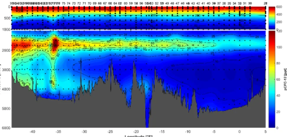
Fig. 5.1. Distribution of SF6 (upper panel) and CFC-12 (lower panel) partial pressure along the equator.
Preliminary results: The distribution of CFC-12 and SF6 along the equator describes the specific ventilation pattern of the different water masses (Fig. 5.1). The main difference in the distribution of both tracers is due to their different atmospheric histories so that CFC-12 already covers the deeper and less ventilated water masses. The shallow and intermediate water masses show the characteristic tracer gradients from equilibrated concentrations at the surface, which monotonically decline towards the Antarctic Intermediate Water (AAIW) at ~800 m. The first tracer minimum and thus less ventilated water layer at ~1000m originates from upper North Atlantic Deep Water (NADW), followed by a significant tracer maximum between 1300-2000 m originating from highly ventilated Labrador Sea Water (LSW). The deep water is dominated by only little ventilated lower NADW. The bottom water along the Romanche Fracture Zone and along the western boundary shows Denmark Strait Overflow water (DSOW). The elevated CFC- 12 and SF6 concentrations in the bottom water indicate the cold and dense Antarctic Bottom Water (AABW).
5.7.2 Underwater Vision Profiler (Rainer Kiko)
During all regular CTD casts, an Underwater Vision Profiler 5 HD (UVP5 HD; serial number 210) was operated on the CTD rosette. The instrument consists of one down-facing HD camera in a 6000 dbar pressure-proof case and two red LED lights which illuminate a 1.24 L-water volume.
During the downcast, the UVP5 takes 20 pictures of the illuminated field per second. For each picture, the number and size of particles are counted and stored for later data analysis. Furthermore, images of particles with a size > 500 µm are saved as a separate “Vignettes” - small cut-outs of the original picture – which allow for later, computer-assisted identification of these particles and their grouping into different particle, phyto- and zooplankton classes. Since the UVP5 was integrated in the CTD rosette and interfaced with the CTD sensors, fine-scale vertical distribution of particles and major planktonic groups can be related to environmental data. In total 102 UVP5 profiles could be obtained. At each station with a water depth < 6000 m a full-depth profile was obtained. Further, computer-assisted analysis of the approximately 750000 images taken with the UVP5 will be done in the home laboratory in order to reveal fine-scale distribution patterns of particles and zooplankton.
5.7.3 Underwater Microscope (Rainer Kiko)
A continuous particle imaging and classification system was operated on the CTD-Rosette during the first 26 CTD profiles obtained off Angola. Pressure-related problems thereafter forced us to deploy the CPICS only down to 110 m depth. We therefore mounted and deployed the CPICS separately, packaged with a Seabird CTD (Table 7.6). The CPICS is an underwater microscope that allows to image plankton and particles in the size range of about 30 µm to 1 mm. Detailed image analysis will be conducted in the home laboratory using deep-learning image recognition algorithms to annotate the recovered images.
5.7.4 Acoustic Zooplankton and Fish Profiler, Mulitnet (Airam Nauzet Sarmiento Lezcano, Rainer Kiko)
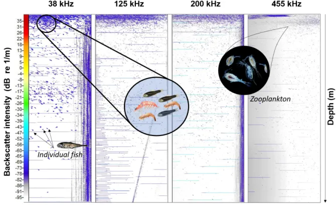
The Acoustic Zooplankton and Fish Profile (AZFP) was used for monitoring the presence and abundance of zooplankton and fish within the water column by measuring acoustic backscatter.
This instrument was mounted on the CTD rosette with the 4 transducers (38, 125, 200 and 455 kHz) oriented towards the side of the rosette. The AZFP was configurated to detect different organisms on the down and upcast, in order to obtain the highest number of detections. The Echoview software and the python Echopype package were used to check the data collected and to get some preliminary results (Fig 5.2). A total of 96 profiles were collected (20 casts between Namibia to Angola and 76 along to the equator). The depth range was variable, reaching a maximum depth near 6000 m. Finally, we will analyze the different frequency profiles (38 kHz for fishes and 125, 200 and 455 kHz for zooplankton) to obtain the vertical distribution of different organisms in the water column and estimate their abundance and biomass.
Fig. 5.2. Fish (38 kHz) and zooplankton (125, 200 and 455 kHz) echogram from the surface to 2500 m depth for one station on the equator.
5.7.5 Nutrient measurements
(Ajit Subramaniam, Rainer Kiko, Gerd Krahmann)
A total of 494 samples were collected for nutrient analysis from CTD casts. The samples were collected in 14 ml polyethylene sampling tubes and immediately frozen for later analysis using an autoanalyzer. While the focus of the nutrient sampling was to define the nutricline, samples from deeper depths were also collected to both serve as reference measurements and to study long term change. In addition, 221 samples were analyzed for NH4 concentrations onboard the ship.
A miniature UV spectrometer (type OPUS manufactured by TriOS) was attached to the CTD during most casts. The spectrometer measures in situ the absorption of UV light by seawater. From comparison with the absorption of clear water and water with a known concentration of nitrate, the nitrate concentration in the seawater sample can be derived. No established processing routines were available during M158. Simple checks showed that the OPUS (#71F9) was properly recording spectra from which the nitrate concentration could be calculated. During the subsequent cruise M159 the same instrument was in use and a processing toolbox was developed based on an existing one for SUNA spectrometer (a similar instrument manufactured by a different company).
Initial processing indicates that the OPUS worked fine during the whole cruise and that nitrate concentrations can indeed be derived. These concentrations still require a calibration comparable to that of the CTD’s conductivity and oxygen sensors. The calibration will be finalized once the frozen nutrient samples have been analyzed. Further improvements of the OPUS processing might be possible by comparing its data with results from the Ocean Optics spectrometer (see section 5.7.8).
5.7.6 Biogeochemistry of nitrous oxide (N2O)
(Sonja Gindorf, Damian Leonardo Arévalo-Martínez)
During TRATLEQ 1, we aimed to investigate the zonal variability of N2O sea-air-fluxes along the equator and to assess the role of variable primary production and sinking organic matter for the cycling of N2O throughout the water column. To this end, we carried out extensive water sampling both from surface waters (every 6 h) and the water column (29 stations spanning surface mixed layer to bottom) in order to measure concentrations of dissolved N2O. Moreover, in order to identify the main processes responsible for N2O production and their variability across the oxygen gradients in the water column, we also collected samples for analysis of N2O isotope signatures. The measurements of N2O concentrations will take place at the Chemical Oceanography Department of GEOMAR, whereas the isotopic analysis will take place at the Marine Stable Isotope Biogeochemistry at the University of South Carolina (USA). Together with oxygen, nutrients, primary production and particle distribution data, we aim to provide the first comprehensive view of the along-equatorial distribution and production of N2O in the Atlantic Ocean.
5.7.7 N2 Fixation, Primary productivity
(Ana Fernández Carrera, Ajit Subramaniam)
Primary production in size fractions was measured at 51 stations (Table 7.7) using two tracer techniques: the radiocarbon (14C) technique (Steeman-Nielsen 1952) and the 13C technique (Hama et al. 1983). The latter was coupled to the 15N2 technique (Montoya et al. 1996) for the estimation of size-fractionated N2 fixation and carbon uptake of the planktonic community in the same incubation bottles. Briefly, for the 14C technique, at each station 1 dark and 3 clear 72 ml polystyrene bottles were filled per depth from 4 depth distributed through the lit upper layer (i.e., euphotic zone) of the water column, spiked with 10µCi of NaH14CO3 and incubated on deck in a system of re-circulating water simulating in situ PAR levels from dawn to dusk on deck. Incubation was terminated sequentially filtering the whole volume of the bottle though 10, 2 and 0.2 µm pore size filters. Then filters were treated on board and the radioactivity was measured in the ship’s Tricarb 2910 scintillation counter. For the 13C/15N2 technique, at each station, triplicate 4.4-L clear polycarbonate bottles (Nalgene) were filled from 2-3 depth, directly from the CTD rosette, spiked with 3 ml of 15N2 (98 atom%, Cambridge Isotopes) and 250 µL of 13C-bicarbonate (0.2M).
Incubation and filtration were similar to that of 14C. The abundance of C and N isotopes in incubated and natural abundance samples will be measured by continuous-flow isotope-ratio mass spectrometry (CF-IRMS) ashore.
5.7.8 HPLC, flow cytometry, photophysiology (Jonathan Joseph Sherman, Ajit Subramaniam)
Samples were collected for enumerating bacterial, cyanobacterial, and picoeukaryote abundance (Table 7.7) and frozen in liquid nitrogen until analysis ashore using a BD Influx flow cytometer following the methods described in (Duhamel et al. 2014).
Phytoplankton functional groups will be determined by High Performance Liquid Chromatography (HPLC) of samples collected throughout the upper 100m at the stations indicated
in Table 7.7. Three liters of water were collected from the Niskin bottles fired at various depths in the euphotic zone and filtered through a GF/F filter. The filters were frozen in liquid nitrogen till analysis. The samples will be analyzed following the method of van Heukelem and Thomas (2001) at the NASA GSFC sample analysis facility.
Phytoplankton photophysiology was assessed using a Fluorescence Induction and Relaxation (mini-FIRe) instrument in combination with a Picosecond Lifetime Fluorescence (PicoLiF) instrument, both custom-built at Rutgers University. The mini-FIRe and PicoLiF use flow-through cuvettes, connected to the ships’ seawater pump to measure continuously from the surface waters along the cruise track at high temporal resolution. System setup included seawater passing through two de-bubblers prior to measurement in order to reduce the effect of bubbles on fluorescence measurements. For a detailed description of methods refer to Lin et al. (2016) and Park et al.
(2017), where the same setup was used. Data collection started on Sep. 19, 2019 at 20:40 and continued almost continuously until Oct. 23, 2019 at 13:30. Each day data collection was stopped in order to download data files for processing, to clean cuvettes, using 90% ethanol, and to collect a blank measurement. A blank sample was prepared by filtering seawater using a 0.2 µm filter. In addition, the mini-FIRe was used to conduct vertical profiles from the CTD casts. During these measurements underway data collection was paused. For vertical profiles, 50 ml of seawater was taken from Niskin bottles in the first 100m for standard measurements as well as blank samples from the surface and the deepest depth sampled for the mini-FIRe. In total 57 depth profile were taken (371 discrete measurements) at the 11ºS section off Angola and the equatorial section.
5.7.9 Organic matter
(Markel Gómez Letona, Alba Filella, Javier Arístegui)
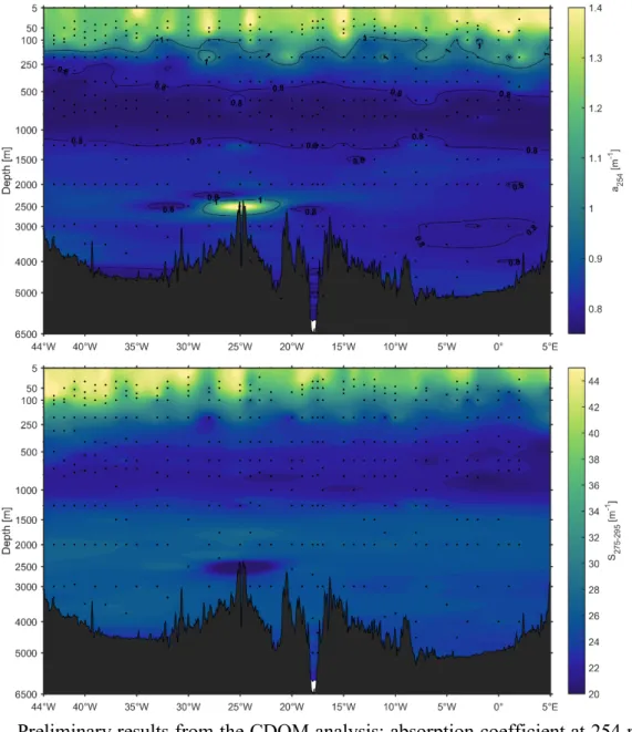
Sampling and analysis: The sampling for the study of the organic matter consisted in samples for Total Organic Carbon (TOC), Particulate Organic Carbon and Nitrogen (POC & PON) and Chromophoric Dissolved Organic Matter (CDOM). Samples for these variables were collected at 63 profiles at 12 depths, from surface to bottom, including the 11ºS section off Angola, the Congo river outflow plume and the equatorial section (Fig. 5.3), for a total of 537 samples.
TOC samples were collected in topaz bottles and were distributed (10 ml, 2 replicates per depth) into high density polyethylene bottles after rinsing. All samples were acidified with 50 µl of phosphoric acid (50%) and stored at -20ºC. TOC samples will be analyzed after the cruise. Samples for POC & PON were filtered through precombusted (450ºC, 6h) glass microfiber GF/F filters.
Upon filtration, filters were placed in individual, precombusted aluminum paper envelopes and stored at -20ºC. POC & PON samples will be analyzed after the cruise.
CDOM samples were collected in topaz bottles for in situ analysis with an Ocean Optics USB2000+UV-VIS-ES Spectrometer alongside a WPI liquid waveguide capillary cell (LWCC).
Samples from the upper 200 meters of the water column were prefiltered using precombusted (450ºC, 6h) glass microfiber GF/F filters to avoid light dispersion by particles. For each sample, absorbance was measured across a wavelength spectrum between 178 nm and 878 nm, performing a blank measurement prior to each sample using ultrapure milli-Q water. Data processing was performed as follows:
1. Data files (samples and blanks) were cropped so as to only preserve wavelengths between 250 and 700 nm.
2. Blank correction: blank spectra were subtracted from sample spectra.
3. Dispersion correction: the average absorbance between 600 and 700 nm was subtracted from the whole spectra.
After processing, absorbance was transformed into absorption following the definition of the Napierian absorption coefficient:
𝑎" = 2.303 ·𝐴𝑏𝑠"
Where, for each wavelength l, the absorption coefficient a𝐿 l is given by Absl (the absorbance at wavelength l), L (the path length of the cuvette, in meters; the LWCC has a length of 0.9982 m) and 2.303, the factor that converts from decadic to natural logarithms.
From the al spectra, several specific wavelengths of interest were considered, mainly al at 254, 325, 354 and 370 nm. Furthermore, spectral slopes between wavelengths of interest were estimated following Helms et al. (2008).
Preliminary results: CDOM results obtained during the cruise present some interesting patterns. Surface waters show an overall decrease in a254 (a proxy for DOM) from east to west in the equatorial Atlantic (Fig. 5.3, upper panel), suggesting a decrease in DOM related to lower productivity in the western basin. However, this overall decrease is not linear, and patches of alternating higher/lower a254 can be appreciated. A preliminary study of this data in combination with meridional velocity data from the ADCP suggests that this patchiness can be related to the northward/southward advection of surface water across the equator due to tropical instability waves. The spectral slope between 275-295 nm (S275-295), which is inversely related to molecular weight of DOM, also shows this patchiness (Fig. 5.3, lower panel).
As expected, a254 decreases with depth as a consequence of the production of DOM by phytoplankton in the surface layer and the recycling and remineralization of DOM by prokaryotes throughout the water. Nonetheless, patterns among these low values can also be discerned, mostly related to the different water masses present in the equatorial region. Minimum a254 values were measured between ~600-1000 m depth and are associated to the Antarctic Intermediate Water (AAIW), which is also present in S275-295, suggesting low concentrations of high-molecular weight DOM as a result of greater remineralization by prokaryotes. This result would agree with the fact that the AAIW is an older water mass than the surrounding waters. Below the AAIW, higher values of a254 were registered in the North Atlantic Deep Water (NADW), although the eastern basin presented lower values than the western. Finally, in the bottom of the western basin, another minimum of a254 was present, a signal associated to the Antarctic Bottom Water (AABW).
Finally, at 25ºW anomalously high values of a254 were measured in most of the deep samples (S275-295 also showed an analogous pattern). A comparison with the UVP5 data showed that these values can be considered real and are associated with high particle abundance. We suggest that this signal stems from hydrothermal activity.