Processes Controlling Stratospheric Dynamic Variability, the Implications for Ozone Levels, and the Coupling to the Troposphere and Mesosphere

(1)

Processes Controlling Stratospheric Dynamic Variability, the Implications for Ozone Levels,

and the Coupling to the Troposphere and Mesosphere

Dissertation

in fulfillment of the requirements for the Degree of Doctor of Natural Sciences

(Dr. rer. nat)

to theFaculty of Mathematics and Natural Sciences of theChristian-Albrechts-Universität zu Kiel

by

Sandro W. Lubis

Kiel, 2016

First Referee: Prof. Dr. Katja Matthes Second Referee: Prof. Dr. Nili Harnik

(2)

ii

Date of the oral examination: 27.06.2016 Approved for publication: 27.06.2016

Signed: Prof. Dr. Wolfgang J. Duschl, Dean

(3)

iii

“The fear of the LORD is the beginning of knowledge, but fools despise wisdom and instruction.”

(Proverbs 1:7)

(4)

(5)

v

Abstract

Stratospheric variability plays an important role in driving the weather and climate of the Earth system. The extent to which various forcing factors explain this variability and the involved mechanisms are not fully understood. This thesis investigates processes controlling the variability of the stratosphere and the implication of this variability on ozone and on circulations in the troposphere and mesosphere. A series of sensitivity simulations with NCAR’s CESM1(WACCM) model was performed to understand how these coupling processes are influenced by different natural and anthropogenic factors. The focus of this thesis is mainly on new aspects of the stratosphere-troposphere coupling mechanism via downward wave coupling (DWC), which is the most direct way by which the stratospheric background wind can affect tropospheric circulation.

Based on a series of sensitivity simulations, it is shown that although DWC is suppressed in the absence of the Quasi-Biennial Oscillation (QBO) variability, the tropospheric signal to DWC is enhanced, and vice versa when the sea surface temperature (SST) variability is excluded. This apparent mismatch is explained by the differences in the strength of the synoptic-scale eddy-mean flow feedback and the possible contribution of SST anomalies during DWC events. In particular, a weaker eddy-mean flow feedback in the absence of SST variability is consistent with modest Eady growth rate and synoptic wave source anomalies, which results in decreased synoptic-scale wave divergence. For the first time, the downward influence of DWC on the surface weather is suggested to be related to enhanced baroclinic instability in the troposphere.

This thesis also provides the first evidence for an effect of DWC on Arctic stratospheric ozone.

A statistically significant decrease in Arctic column ozone is observed towards late winter during years with enhanced DWC. This is attributed to an increased net amount of wave reflection that leads to a cold polar vortex and less ozone transport to the pole. The results establish a new perspective on dynamical processes controlling Arctic ozone variability.

Under extreme climate change conditions, a significant reduction in DWC events is detected in the future, with a shift of their timing from early to midwinter. This variation is related to changes of the vertical reflecting surfaces and an increased wave absorption in early winter. The result also indicates that future changes in midwinter surface weather during DWC event are related to changes in baroclinic eddy feedback in the troposphere.

In the last part of this thesis, the impact of the Antarctic ozone hole on the vertical coupling of the stratosphere and mesosphere-lower thermosphere (MLT) system is investigated in detail. The results highlight that a proper accounting of both, dynamical and radiative effects, is required in order to correctly attribute the causes of the polar MLT response to the Antarctic ozone hole.

This thesis provides an advanced understanding of the mechanisms responsible for the coupling between the troposphere, stratosphere, and beyond in both the upward and downward directions. This knowledge has the potential to improve the representation of middle atmosphere circulation in climate models, and thus to improve predictions of ozone, climate, and even tropospheric weather.

(6)

vi

Zusammenfassung

Die Variabilität in der Stratosphäre spielt eine wichtige Rolle für das Wetter und Klima des Erdsystems. Welche unterschiedlichen Faktoren diese Variabilität beeinflussen und wie diese zu den physikalischen Mechanismen beitragen, ist bisher nicht vollständig verstanden und Gegen- stand dieser Arbeit. Außerdem werden die Auswirkungen der stratosphärischen Variabilität auf die Ozonkonzentration und auf die Zirkulation in der Tropo- und Mesosphäre untersucht. Um den Einfluss verschiedener natürlicher und anthropogener Faktoren auf diese Kopplung besser zu verstehen, wurden verschiedene Sensitivitätsexperimente mit NCAR’s Erdsystemmodell, CESM1 (WACCM), durchgeführt. Der Fokus dieser Arbeit liegt hauptsächlich auf neuen Aspekten der Stratosphären-Troposphären Kopplung durch abwärts gerichtete Wellenkopplung (DWC, von engl.: downward wave coupling). Abwärts gerichtete Wellenkopplung ist der direkteste Weg, über den stratosphärische Winde die Zirkulation in der Troposphäre beeinflussen können.

Mit Hilfe dieser Sensitivitätsexperimente wird gezeigt, dass das troposphärische Signal, wel- ches auf DWC-Ereignisse folgt, ohne das Vorhandensein einer quasi zweijährigen Schwingung der tropischen Winde in der Stratosphäre verstärkt wird, obwohl die abwärts gerichtete Wellen- kopplung schwächer ist. Bei fehlender Variabilität der Meeresoberflächentemperaturen hingegen verhält es sich genau umgekehrt. Dieser scheinbare Widerspruch wird auf die unterschiedlich starke Wechselwirkung von synoptischen Wellen mit dem Grundstrom sowie auf einen möglichen Einfluss der Variabilität der Meeresoberflächentemperatur während eines DWC-Ereignisses zu- rückgeführt. Eine schwächere Wechselwirkung zwischen synoptischen Wellen und dem Grund- strom bei fehlender Variabilität der Meeresoberflächentemperatur steht im Zusammenhang mit einer geringeren Eady-Wachstumsrate und mit Anomalien im Auftreten von Quellen synoptischer Wellen. Dies resultiert in verringerter Divergenz synoptischer Wellen. Zum ersten Mal wird der abwärts gerichtete Einfluss von Wellenkopplung auf das Wetter mit verstärkter barokliner Instabilität in der Troposphäre in Zusammenhang gebracht.

Erstmals wird in dieser Arbeit der Einfluss von abwärts gerichteter Wellenkopplung auf die Ozonkonzentration in der arktischen Stratosphäre untersucht. In Jahren mit erhöhter Anzahl von DWC-Ereignissen wird eine statistisch signifikante Abnahme in der Ozonkonzentration zum Ende des Winters beobachtet. Dies wird auf eine erhöhte Gesamtanzahl von Wellenreflektionen in der Stratosphäre zurückgeführt, welche zu einem kalten Polarwirbel und zu einem verringerten Trans- port von Ozon in Richtung Pol führen. Diese Ergebnisse ermöglichen eine neue Perspektive in Hinblick auf die dynamischen Prozesse, die die Variabilität von arktischem Ozon bestimmen.

Unter Verwendung eines extremen Klimawandelszenarios wird eine Abnahme der DWC- Ereignisse in der Zukunft bei gleichzeitiger zeitlicher Verschiebung des Auftretens dieser Ereignisse zur Mitte des Winters festgestellt. Dies wird auf Veränderungen der vertikalen Reflektionsflächen und erhöhte Wellenabsorption zurückgeführt. Die Ergebnisse lassen außerdem darauf schließen, dass zukünftige Änderungen des Winterwetters während DWC-Ereignissen mit Änderungen der baroklinen Wellenwechselwirkungen in der Troposphäre in Zusammenhang stehen.

(7)

vii Im letzten Teil dieser Arbeit wird der Einfluss des antarktischen Ozonlochs auf die vertikale Kopplung von der Stratosphäre in die Meso- und untere Thermosphäre (MLT, von engl.: mesosphere and lower thermosphere) im Detail untersucht. Die Ergebnisse machen deutlich, dass eine Berücksichtigung von Strahlungs- und dynamischen Effekten für die Auswirkungen des antarktischen Ozonlochs auf die MLT notwendig ist.

Diese Arbeit liefert ein vertieftes Verständnis der dynamischen Prozesse, welche für die abwärts und aufwärts gerichtete Kopplung zwischen Troposphäre, Stratosphäre und höheren Atmosphärenschichten von Bedeutung sind. Dieses Wissen hat das Potential, die Repräsentation der mittleren Atmosphäre in Klimamodellen zu verbessern und damit bessere Klima-, Ozon- und Wetterprognosen zu ermöglichen.

(8)

(9)

ix

Atmospheric layers are coupled vertically by radiative, dynamical, and chemical processes acting on different timescales. These couplings do not only comprise atmospheric processes, but also include interactions with other components of the Earth’s systems, such as ocean, sea-ice, and land surface. For example, changes in the chemical composition of radiatively active gases, such as ozone (O3) in the stratosphere cause significant changes in stratospheric temperatures as well as surface radiative forcing (e.g., Ramaswamy et al. 2001). On the other hand, variations in the stratospheric polar vortex induced by the variation in solar ultraviolet radiation could influence the tropospheric circulation by modifying vertically propagating planetary waves (e.g., Geller and Alpert1980). Although these three coupling processes are equally important for the climate system, this thesis focuses mostly on the dynamical coupling mechanisms between the troposphere, stratosphere, and higher layers in both the upward and downward directions.

The dynamical coupling between the troposphere and stratosphere is primarily driven by a two-way interaction between atmospheric waves and the mean flow. Planetary waves originating from the troposphere propagate upward into the stratosphere, where they interact with the polar vortex. In extreme cases, the breaking or dissipating waves exert a systematic mean force that leads to a destruction of the polar vortex, causing a sudden stratospheric warming (SSW) event.

SSWs evolve downwards into the troposphere where they can affect surface weather and climate (e.g., Baldwin and Dunkerton2001; Limpasuvan et al.2004). During periods following a sudden warming, studies have shown that a knowledge of the winds in the stratosphere increases predictability of the troposphere (e.g., Baldwin et al.2003; Kuroda2008). On the other hand, upward propagating planetary waves into the stratosphere can also be reflected back down to the troposphere, resulting in downward planetary wave coupling (DWC, Perlwitz and Harnik2003).

DWC has been found to significantly affect the tropospheric weather and surface climate over the North Atlantic sector (e.g., Shaw and Perlwitz,2013; Dunn-Sigouin and Shaw,2015; Lubis et al., 2016b). However, the underlying physical mechanisms that affect the variability of DWC and the associated impact on the troposphere are far from being fully understood. Thus, a better understanding of dynamical stratosphere-troposphere coupling via planetary wave coupling processes is required to improve predictions of tropospheric weather and climate.

Several studies have linked variations in stratospheric weather phenomena to the temperature and circulation changes in the mesosphere through gravity wave modulation (Smith et al., 2010; Lossow et al., 2012). Smith et al. (2010) showed that the ozone-hole-induced changes in

(12)

2 Chapter 1. General Introduction the stratospheric wind field leads to a warming of the polar summer mesopause, as a result of enhanced westerly gravity wave drag filtering. Other studies showed that enhanced easterly gravity wave drag filtering in the stratosphere during SSW events leads to a polar mesospheric cooling (analogous to the ozone hole’s impact but with an opposite sign) [e.g., Walterscheid et al.2000; Liu and Roble2002; Hernandez 2003; Cho et al.2004]. However, there are still gaps in our knowledge about the importance of planetary wave forcing for the stratosphere-mesosphere coupling. Thus, a better knowledge of dynamical stratosphere-mesosphere coupling and the involved mechanisms will help to improve the representation of mesospheric circulation in climate models.

The goal of this thesis is to investigate various aspects of the variability of the stratospheric polar vortex and the effect of this variability on ozone and circulations in the troposphere and mesosphere. The first part of this thesis investigates the stratospheric-troposphere coupling mechanism via downward planetary wave reflection. This includes investigation of the effects of different natural and anthropogenic factors on the variability of DWC, the impact of DWC on polar stratospheric ozone, and the underlying mechanism responsible for the tropospheric responses to DWC. In the last part of the thesis, a complete mechanism of the stratosphere-mesosphere-lower thermosphere (MLT) coupling during the Antarctic ozone hole period is proposed. This is the first study that investigates the combined effects of dynamical (resolved and non-resolved wave driving) and radiative forcings on the MLT response to the ozone hole. All underlying physical mechanisms for these couplings will be investigated in this thesis.

1.1 Theory of Vertically Propagating Rossby Waves

Fundamental properties of vertically propagating planetary waves, which is the basis of studies of the dynamical coupling between the stratosphere and the troposphere, are reviewed briefly. On aβ plane, the linearized quasi-geostrophic potential vorticityqin the logarithmic pressure coordinate (z=-H logp), under assumption of conservative flow, can be expressed as follows (Charney and Drazin,1961):

(∂

∂t+ ¯u ∂

∂x)q⁰+ ¯q_y∂ψ⁰

∂y = 0 (1.1)

whereψ = Φ/f is the geostrophic streamfunction, q is quasigeostrophic potential vorticity, Φ is geopotential, and f is the Coriolis parameter. The overbar and prime denote zonal mean and eddies (deviations from zonal mean), respectively. Equation (1.1) has solutions in the form of harmonic waves with zonal and meridional wavenumbers (k and l), respectively, and angular frequencyω:

ψ⁰(x, y, z, t) = Ψ(z)exp

i(kx+ly−ωt) + z 2H

(1.2)

(13)

1.1. Theory of Vertically Propagating Rossby Waves 3 whereΨ is a function only of z. Note that the altitude factor exp(z/2H) takes into account the fact that a propagating non-dissipating wave will conserve energy, which is proportional to|ψ⁰|². Substituting (1.12) to the equation (1.1), yields

d²Ψ

dz² +m²Ψ = 0 (1.3)

where

m² = N² f²

"

¯ q_y

¯ u−Cpx

−(k²+l²)

#

− 1

4H². (1.4)

and zonal phase speedCp = ω/k. We recall that m² must be positive for the vertical propagation, and thus vertically propagating modes can exist only for zonal mean flows that satisfy the following condition:

Cpx<u < C¯ px+ q¯_y k²+l²+ _4N^f2²H²

≡Uc. (1.5)

whereU_c is called as the Rossby critical velocity and H is the density scale height. This condition suggests that stationary (Cpx >0) Rossby waves cannot propagate vertically in the easterlies (Charney and Drazin, 1961). In the westerlies, only the Rossby waves with longer zonal wave- length can propagate vertically in the strong wind speed. If the westerly speed increases with height under condition of constantq¯y, upward propagating waves reaching at some level where

¯

u=U_cfor eachkcannot propagate farther above that level. This can be seen in Fig.1.1, that long waves are able to propagate upward in contrast to high wavenumbers (K > 5). Such waves are already filtered by a moderate zonal wind (U > 20 m/s). This property has a consequence in the seasonal pattern of vertical propagating Rossby waves.

FIGURE 1.1: Vertically propagating Rossby waves as a function of background flow (U) and the total wavenumberKat 50^oN and a buoyancy frequency ofN= 2·10⁻²s⁻¹(see Eq.1.5).

Furthermore, if u¯ satisfies the above condition (1.5), thus Ψmay be written as: Ψ(z) = ψ0

exp(imz), whereψ₀ is a constant andi represents imaginary part. The equation (1.12) becomes

(14)

4 Chapter 1. General Introduction

FIGURE 1.2: A vertically propagating Rossby wave in the NH (warm/cold are reversed in the Southern Hemisphere). Note that this should be multiplied by exp(z/2H) to give the actual result for ψ⁰. Figure adapted from Charney and Drazin,1961.

ψ⁰(x, y, z, t) =ψ₀exp(i(kx+ly+mz) +z/(2H)), for which we obtain a dispersion relation as:

ω= ¯uk− kq¯y

K²+_4N^f2²H

, (1.6)

where

K² =k²+l²+ f₀²

N²m²= q¯y

¯

u−C_px − f²

4N²H². (1.7)

Therefore, the group velocity,C_g = (C_gx, C_gy, C_gz)^T, can be expressed as:

C_gx=C_px+ 2 ¯q_yk²

K²+ (_4HN^f² 2)²; (1.8)

Cgy= 2 ¯qykl

K²+ (_4HN^f²2)²; (1.9)

Cgz = 2_N^f²2q¯ykm

K²+ (_4HN^f²2)²; (1.10)

For stationary waves (Cpx=0), the group velocity may be simplified as:

C_g = (k, l, f²

N²m)× 2¯uk K²+_4HN^f 2

, (1.11)

Thus, the group velocity of a stationary Rossby wave is tangent to phase lines in a horizontal plane, phase lines associated with the upward- (downward-) propagating Rossby wave group velocity are tilted westward (eastward) with height (see schematic diagram in Fig1.2). On the other hand a west-and eastward tilt of the waves with increasing latitude characterizes pole- and

(15)

1.2. Stratosphere-Troposphere Coupling 5 equatorward propagation, respectively. It is also shown that the magnitude of the group velocity is almost twice as large asu¯(i.e., |C_g = 2¯ucosα|), whereαis the angle between lines of constant phase and the y axis .

1.2 Stratosphere-Troposphere Coupling

Recently, the dynamical influence of the stratosphere on the troposphere has been extensively studied due to its implication for extended-range forecasts and climate variability (e.g., Baldwin and Dunkerton2001; Limpasuvan et al. 2004; Kuroda 2008). As a pioneer work for this study, Quiroz (1977) showed that a large increase of temperature anomalies in the troposphere was linked to extreme stratospheric phenomena, SSWs. Through numerical experiments, Geller and Alpert (1980) argued that changes in the tropospheric circulation were attributed to variations in the stratospheric polar night jet (PNJ) through modulation of planetary wave propagation. Likewise, Boville (1984) showed that changes in the stratospheric PNJ could alter the tropospheric circulation by modifying the transmission-refraction properties of vertically propagating waves.

The downward propagation of the stratospheric zonal-mean zonal wind anomalies to troposphere in the NH was firstly shown by Kodera et al. (1990). In that process, the observed westerly anomalies first appear in the upper stratosphere and then propagate downward into the troposphere within a month, accompanied by anomalous meridional propagation of planetary waves (Kodera et al.1990; Kodera et al.1991). Much of the evidence for a stratospheric impact on the troposphere has been widely described using the so-called annular modes: the Northern Annular Mode (NAM) and Southern Annular Mode (SAM) (e.g., Baldwin and Dunkerton1999;

Thompson and Wallace2000). These modes are the dominant patterns of variability in the extra tropical troposphere and stratosphere, characterized by a zonally-symmetric, barotropic dipole pattern between the polar region and mid-latitude in the stratosphere and troposphere winter.

Baldwin and Dunkerton (1999) showed that the NAM anomalies first appear in the stratosphere and subsequently progress downward into the troposphere over periods of a few weeks. Figure1.3 shows composites of weak vortex events from the NCEP-NCAR Reanalysis taken from Baldwin and Dunkerton (2001). It is evident that anomalous values of the NAM are evident in the troposphere and at the surface for up to two months after they first appear in the stratosphere. In the stratosphere the annular mode values are a measure of the strength of the polar vortex, while the near surface is recognized as the "Arctic Oscillation (AO)" or the North Atlantic Oscillation (NAO). Moreover, subsequent studies showed that the best extended-range forecasts of the AO in the winter can be achieved by using the lower stratospheric NAM as a predictor (e.g., Baldwin et al.2003).

While the influence of the troposphere on the stratosphere is well established, the influence in the opposite direction is more difficult to determine. A simple schematic diagram to illustrate the stratospheric downward influence on the troposphere during strong polar vortex conditions is given in Fig1.4(Kidston et al.,2015). First, weaker planetary wave forcing in the stratosphere

(16)

FIGURE1.3: (a) composite of time-height development of the NAM for 18 weak vortex events (top). The contour interval for the colour shading is 0.25 and 0.5 for the white contours. (b) Average sea-level pressure anomalies (hPa) for the 1080 days during weak vortex regimes. Figure from Baldwin and Dunkerton (2001).

leads to strengthening of the polar vortex (1). The reduced stratospheric wave forcing is in turn balanced by the Coriolis force, resulting in upward (downward) residual circulation at high latitudes (mid-to-low latitudes) and subsequent adiabatic cooling (warming) in this region (2). The mass redistribution – through upwelling/downwelling – increases the tropopause heights and reduced mean sea level pressure in polar latitudes and vice versa in mid-latitudes (3). The tropospheric eddy feedbacks (4), in turn, induce and maintain a poleward shift of both the tropospheric jet and the storm tracks (5). Although it is generally recognized that the tropospheric eddy feedbacks are linked to a poleward shift of tropospheric jet, the involved mechanism is not completely clear.

According to the timescales of the process, the stratosphere-troposphere coupling can be distinguished into: (1)short term coupling that includes planetary wave activity: wave absorption (e.g., Matsuno1970; McIntyre and Palmer1983), wave reflection (e.g., Harnik and Lindzen 2001; Perlwitz and Harnik 2003), and wave resonance (e.g., Tung and Lindzen 1979; Esler and Scott2005), (2)intraseasonal couplingincluding downward influence of sudden and final stratospheric warmings (e.g., Baldwin and Dunkerton2001; Limpasuvan et al.2004; Sun and Robinson 2009), and (3)interannual couplingthat includes modification of eddy-mean flow interactions by El Niño-Southern Oscillation (ENSO, e.g., Loon and Labitzke1987; Manzini et al.2006), Quasi- Biennial Oscillation (QBO, e.g., Holton and Tan1980; Coughlin and Tung 2001), solar cycle (e.g., Kodera and Kuroda2002; Matthes et al.2006), volcanoes (e.g., Robock and Mao1992; Fischer et al.2007), sea-ice changes (e.g., Jaiser et al.2013), Atlantic meridional overturning circulation (e.g., Reichler et al.2012) etc.

The exact dynamical mechanism by which the stratospheric signals can be transmitted to the

(17)

1.2. Stratosphere-Troposphere Coupling 7

FIGURE 1.4: A sketch of stratospheric downward influence during a strong vortex event. Figure from Kidston et al. (2015).

troposphere and surface, however, is unknown, but a number of theories have been proposed. The first theory is a direct adjustment of the tropospheric flow to stratospheric potential vorticity (PV) anomalies (diagnosed by PV inversions; Hartley et al.1998; Ambaum and Hoskins 2002; Black 2002). This theory explains how tropospheric wind anomalies can be influenced by stratospheric potential vorticity. In particular, enhanced positive stratospheric PV anomalies associated with a strong stratospheric polar vortex cause both a rise of the tropopause height and stretching of the tropospheric column. This results in lower pressure levels in polar latitudes and increase of the tropospheric westerlies (Ambaum and Hoskins2002). An equivalent mechanism to the non- local effect of the PV inversion is the "downward control" principle (Haynes et al.1991; Holton et al. 1995). This mechanism shows that the meridional circulation is non-locally controlled by wave induced forcing. In other words, the meridional circulation at each level is controlled only by the forces acting above it. Another idea includes changes in refractive properties and Rossby wave propagation (Hartmann et al.2000; Limpasuvan and Hartmann2000). In this mechanism, changes in the vertical structure of stratospheric winds (shear and curvature) cause changes in transmission and refraction properties of vertically propagating waves. The last mechanism is associated with the downward reflection of wave activity by the stratosphere back into the troposphere (e.g., Perlwitz and Harnik2003).

Recent model and observational studies also reported the importance of synoptic eddies in shaping and maintaining the downward influence of stratospheric anomalies in the troposphere (e.g., Limpasuvan et al.2004; Song and Robinson2004; Simpson et al.2009; Kunz and Greatbatch 2013; Domeisen et al. 2013). In particular, Simpson et al. (2009) performed spin-up experiments with an idealized general circulation model (GCM) by looking at the response to many different stratospheric forcings and reported that changes to eddies are related to changes in the refractive

(18)

8 Chapter 1. General Introduction index near the tropopause. Other studies also reported that changes in the mean flow conditions in the vicinity of the tropopause, can affect synoptic eddies in the troposphere via changes in lower stratospheric shear (Wittman et al., 2007), isentropic slope (Thompson and Birner, 2012), eddy length scale (Kidston et al., 2010), and eddy phase speed (Chen and Held, 2007). However, the direct impact of planetary wave coupling on synoptic scale eddies in the troposphere is still not fully understood.

In this thesis, the mechanism of stratosphere-troposphere dynamical coupling via downward planetary wave reflection is investigated in detail. Planetary waves are generated in the troposphere by orographic and non-orographic forcing (diabatic heating and/or interaction with transient eddies) (e.g., Kuroda and Kodera1999; Kodera and Kuroda2000; Baldwin and Dunker- ton2001; Christiansen2001; Plumb and Semeniuk2003; Polvani and Waugh2004). These waves propagate upward into the stratosphere where they either dissipate or are reflected downward toward the troposphere, resulting in downward wave coupling.

1.3 Downward Wave Coupling (DWC)

Although a mechanism of a downward dynamic influence – reflection of wave activity by the stratosphere back into the troposphere – has been suggested by several authors in the past (Hines 1974; Geller and Alpert 1980; Schmitz and Grieger 1980; Bates1981), Perlwitz and Harnik (2003) was the first to clearly show the impact of reflected wave-packets on tropospheric planetary waves.

In this section, the fundamental properties of DWCs and their effects on the tropospheric circulation are reviewed.

1.3.1 Fundamental Properties of DWC

DWC occurs when the upward propagating waves decelerate the polar vortex in the upper stratosphere, causing the formation of a reflecting surface that redirects waves back to the troposphere (Harnik and Lindzen2001; Lubis et al.2016b, see also Fig1.5). The reflecting surface forms as a result of the negative vertical westerly shear that leads to negative meridional PV gradient (see Eq.1.12). When the zonal mean winds decrease with height in the upper stratosphere, the index of refraction squared for these waves becomes negative, blocking the waves from propagating further up. As a result, the waves are reflected back down to the troposphere, instead of being absorbed in the stratosphere (Harnik and Lindzen,2001; Perlwitz and Harnik,2003; Lubis et al.,2016b), leaving the vortex strong and the pole cold. Harnik (2009) showed that a lower stratospheric acceleration also contributes to this negative vertical shear, and that this acceleration occurs at the trailing edge of the upward pulse of wave activity. Thus, reflection is associated with short wave forcing, while SSWs are associated with long wave pulses (e.g., Harnik2009; Sjoberg and Birner 2012), which are often manifested as blocking events (e.g., Quiroz1986; Naujokat et al. 2002; Woollings et al.

2010). The meridional PV gradient, which is an important ingredient for the formation of vertical

(19)

1.3. Downward Wave Coupling (DWC) 9

FIGURE 1.5: (a) The squared covariance between Z-ZWN1500 and Z-ZWN110 calculated from the time- lagged SVD analyses for negative (reflective) or positive (non-reflective) U2−10 index in JFM. A positive (negative) time lag indicates that the stratospheric (tropospheric) wave field is leading. (b-c) The composites of vertical and meridional wavenumbers, calculated for each of the reflective and non-reflective years. Gray shading indicates regions of wave evanescence in the meridional (l < 0) and vertical (m < 0) directions.

Data was obtained from ERA reanalysis. See Chapter2for a detailed methodology description.

reflecting surface, can be approximately written as:

q_y ≡β− 1 a²

∂

∂φ

1

cosφ

∂(ucosφ)

∂φ

− f²

HN² + f² N⁴

∂N²

∂z

!∂u

∂z + f² N²

∂²u

∂z². (1.12) whereN²is the buoyancy frequency, andβis the variation of the Coriolis parameter with latitude.

The third term of the right hand side can be negative associated with a decreasing zonal-mean zonal wind speed with height. Hence, this quantity contributes to decreasing total wavenumber K(see Eq.1.7) to yield m=0 (reflecting surface).

Perlwitz and Harnik (2003, 2004) showed that NH winters tend to be either reflective (very cold and undisturbed), or non-reflective (absorptive, with a SSW), with the two occurring approximately equally in the observational record. In the non-reflective state, most of the waves gets deposited in the stratosphere, resulting in strong wave-mean-flow interaction, while in the other state, wave activity is reflected back down to the troposphere resulting in more DWC events and affecting the structure of tropospheric planetary waves (Fig1.5). The reflective state is characterized by a well-defined high-latitude meridional waveguide in the lower stratosphere that is bounded above by a vertical reflecting surface (Fig1.5). This configuration is favourable for the occurrence of DWCs and known as bounded wave geometry. The bounded wave geometry can be diagnosed by determining the existence and location of turning surfaces for meridional and vertical propagation. For a non-isothermal atmosphere, a general refractive index (n²_r) decomposition for waves with a zonal wavenumberkand a phase speedc, is written as (for details, see Harnik and Lindzen2001and Chapter2):

(20)

n²_r ≡ N² f²

( q¯_y

u−c−k²+f²e^z/2H N

∂

∂z

"

e^−z/H N

∂

∂z

e^z/2HN

#)

≡m²+N²

f² l². (1.13) From (1.13), the waves propagate in the vertical (meridional) direction whenm² >0(l² > 0), are evanescent whenm² <0(l² <0), and are reflected whenm² = 0(l² = 0).

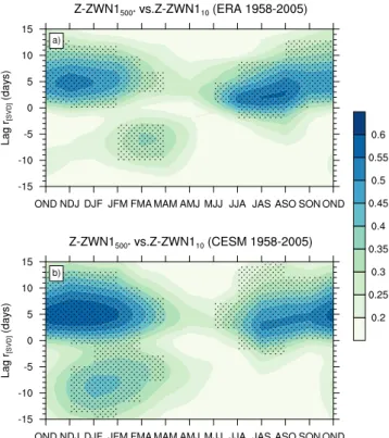
FIGURE1.6: Three-month overlapping periods of lagged SVD correlations between Z-ZWN1 at 500 hPa and 10 hPa calculated from ERA reanalysis for (a) NH and (b) SH. Black dots represent statistically significant values at the 99% level calculated using a Monte Carlo approach (see Chapter2for a detailed methodology description).

In the NH, the formation of bounded wave geometry happens intermittently, when waves decelerate the vortex only in the upper stratosphere. However, in the SH this happens every year towards the end of winter, as part of the seasonal cycle (Shaw et al., 2010). In Figure 1.6, the seasonal cycles of DWC in the Northern and Southern Hemispheres are presented by time-lagged singular value decomposition (SVD) correlations between geopotential height wave number 1 (Z- ZWN1) at 500 hPa and 10 hPa from ERA reanalysis. A negative (positive) time lag indicates that the stratospheric (tropospheric) wave field is leading. Therefore, the most favourable season for DWCs in the NH is during midwinter from January to March, while in the SH it occurs from September to December (Fig1.6).

Although the mechanism by which tropospherically forced waves are reflected downwards in the stratosphere is already well established, what factors determine the variability and the source of DWCs remains a difficult question, and is one of subjects of this thesis. In this thesis, the influence of different natural and anthropogenic forcing factors on the DWC variability was investigated using a unique set of model simulations, which include both an interactive ocean and an interactive chemistry module, extending up to the thermosphere.

(21)

1.3. Downward Wave Coupling (DWC) 11 1.3.2 Tropospheric Impact of DWC

DWC is the most direct way by which the stratospheric background wind can affect tropospheric circulation. Recent studies have revealed that the wintertime distribution of high-latitude planetary wave-1 heat flux exhibits extreme values that are linked to the tropospheric circulation in the North Atlantic (Shaw and Perlwitz,2013; Shaw et al.,2014; Dunn-Sigouin and Shaw, 2015; Lubis et al.,2016b). Shaw and Perlwitz (2013) investigated the dynamics of DWC in the NH using total (anomaly plus climatology) negative wave-1 heat flux values. They showed that the life cycle of DWC in the stratosphere occurred over a few weeks and involved vertical coupling via a clear high-latitude wave-1 pattern in the troposphere that results in a poleward jet shift in the Atlantic sector. The growth of wave-1 amplitude began around the time of minimum heat flux and was followed by the development of a reflecting surface. The associated near-surface temperature and mean sea level pressure anomalies are very reminiscent of the positive phase of the North Atlantic Oscillation (NAO). Subsequent studies by Shaw and Perlwitz (2014) and Dunn-Sigouin and Shaw (2015) showed that extreme positive and negative stratospheric wave-1 heat flux values are instantaneously linked to poleward and equatorward shifts of the tropospheric jet. However, the mechanism by which the DWC affects the tropospheric jet shifts and what factors control the strength of tropospheric response to DWC remain unclear.

The basic principle of the dynamical coupling between stratosphere and troposphere via DWC, as well as the unclear mechanisms related to this coupling process are illustrated in Fig1.7.

FIGURE1.7: A stratosphere-troposphere coupling mechanism via DWC. The red (blue) arrow indicates the direction of the planetary wave propagation. The shaded oval indicates Eliassen-Palm (EP) flux divergence.

The horizontal orange solid line indicates vertical reflecting surface (m² = 0). The effects of the QBO, SST and anthropogenic (GHG and ODSs) forcings on this coupling mechanism are unclear and marked with "?".

Likewise, the mechanisms responsible for downward influence on the troposphere and the implication for ozone levels are not understood.These questions will be answered in this thesis.

(22)

1.4 Impact of Stratospheric Variability on Polar Stratospheric Ozone

Much of the interannual variability in the stratosphere is caused by variations in planetary wave activity, with the amount of ozone depletion strongly correlating with the total amount of wave activity entering the stratosphere from the troposphere during winter (Fusco and Salby,1999; Ran- del et al., 2002; Weber et al., 2003). Randel et al., 2002show that variations in planetary wave forcing in the lower stratosphere during winter-spring exhibit a strong correlation with column ozone. The mechanism for this is that increased (decreased) wave dissipation in the stratosphere leads to strengthening (weakening) of residual circulation, which in turn increases (decreases) the transport of ozone-rich air to the polar lower stratosphere. On the other hand, strong (weak) midwinter planetary wave forcing causes a warmer (cooler) Arctic lower stratosphere in early spring (Newman et al.,2001), resulting in smaller (larger) chemical ozone losses in spring. A recent study by Manney et al. (2011) revealed that the unprecedented Arctic ozone loss in 2011 is highly cor- related with extremely cold lower-stratospheric temperatures in early spring. These extremely low temperatures are attributed to the unusually weak midwinter planetary wave forcing in the stratosphere (Hurwitz et al., 2011), as expected from a close relationship between polar spring temperatures and eddy heat flux in mid to late winter (Newman et al.,2001).

The NH winter stratosphere is characterized by large interannual variability, which either results in very disturbed winters with SSWs, or very cold undisturbed winters. SSWs are dramatic events that cause the stratospheric pole to heat up by tens of degrees within a period of days, and cause the strong winds circulating the pole to reverse direction (e.g., Baldwin et al. 2003;

Kuroda2008). Enhanced stratospheric wave dissipation during SSW events causes strengthening of the residual circulation and a warmer polar vortex. This in turn leads to more dynamical ozone transport to the pole and less springtime ozone destruction (e.g., Rose and Brasseur1985; Randel 1993; Hocke et al.2015). On the other hand, cold and undisturbed stratospheric winters provide opportunity for temperatures to drop below the threshold for the formation of Polar Stratospheric Clouds (PSCs), on which ozone destruction processes take place. In the SH, this results in an ozone hole in the polar stratosphere every spring, the pole being dynamically isolated from lower latitudes by the strong winds that circulate it. The NH pole is not as dynamically isolated as the SH, and winter temperatures do not regularly drop as low, so the degree of ozone destruction is much smaller and more variable from year to year.

Though very different in their type of influence, both of the aforementioned dynamical influences – SSWs and cold winters with low ozone levels – involve the interaction of the polar vortex with planetary waves’ large-scale undulations of the vortex which propagate up from the troposphere, then break and are absorbed in the vortex, slowing it down and heating the pole in the process (e.g., Solomon1999; Fusco and Salby1999; Randel et al.2002). When wave absorption is very strong, a SSW occurs, and when it is very weak, polar temperatures become cold enough for ozone to be destroyed. Since the amount of wave-induced heating in the NH is highly variable, the occurrences of cold winters with ozone depletion, or winters with SSWs, are also highly variable. One process that is associated with reduced wave absorption is DWC (Harnik, 2009).

(23)

1.5. External Forcing Factors Influencing Stratospheric Variability 13 The vortex remains strong and cold when the waves are reflected back down to the troposphere, instead of being absorbed in the stratosphere (Harnik and Lindzen, 2001; Perlwitz and Harnik, 2003). Therefore, winters with increased DWC activity are expected to be related with strong ozone destruction.

In this thesis, the impact of the DWC on stratospheric circulation, polar temperatures, and ozone is investigated in Chapter3. Determining the connection between DWC, residual circulation, and polar temperatures is one of the keys to improving our understanding of the link between stratospheric dynamics and ozone variability both in the real atmosphere and in stratosphere- resolving chemistry-climate models (CCMs). The schematic diagram showing a possible influence of DWC on polar stratospheric ozone is also illustrated in Fig1.7.

1.5 External Forcing Factors Influencing Stratospheric Variability

Variability in the stratosphere is the result of complex and nonlinear relationships between various forcings affecting the evolution of the stratosphere (e.g., Calvo et al. 2009; Richter et al.

2011). Recent studies have shown that understanding the factors influencing the polar vortex can improve tropospheric weather forecasts and seasonal predictions for different latitudes and regions (e.g., Baldwin and Dunkerton2001; Thompson and Solomon2002; Domeisen et al.2015). In addition, it is well established that the two-way vertical (upward and downward) planetary wave propagation, which influence the strength of the polar vortex, can be modified by changes in the vertical and meridional structures of the zonal mean wind (Charney and Drazin1961; Limpasu- van and Hartmann 2000; Perlwitz and Harnik 2003). Therefore, examining which factors affect the variability of the polar vortex can help us understand what processes control the variability of DWC and its associated impact on tropospheric circulation.

The forcing factors influencing stratospheric variability can be distinguished into "natural"

and "anthropogenic" forcings. The natural forcing factors are responsible for natural or internal climate variability (IPCC,2013). These forcings include the QBO of equatorial stratospheric winds, variations in sea surface temperatures (SSTs), volcanic eruptions, and variations in solar radiation.

Many studies have shown that these natural forcing factors have significant impact on the variability of the polar vortex (e.g., Holton and Tan1982; Loon and Labitzke1987; Labitzke and Loon 1996; Matthes et al. 2006). Recent studies with CCMs have also shown the QBO and SSTs play important roles for representation of mutually dynamical relations between the stratosphere and troposphere in climate models (e.g, Calvo et al.2009; Richter et al.2011; Hansen et al.2014; Lubis et al.2016b). On the other hand, anthropogenic forcings are human-induced factors that include greenhouse gases (GHG, prominent examples are carbon dioxide (CO2) and methane (CH4)) and ozone-depleting substances (ODS, e.g, chlorofluorocarbons). Changes in GHG and ODS concentrations in the atmosphere have been reported to significantly influence the climate system. Under increased GHG emissions, a globally averaged tropospheric warming and stratospheric cooling are expected (e.g., Bell et al.,2010a; IPCC,2013; Marsh et al.,2013). Increased ODSs that lead to the

(24)

14 Chapter 1. General Introduction ozone hole, on the other hand, has caused a significant climate change in the SH during the last three decades (e.g., Gillett and Thompson2003; Marsh et al.2013).

In this thesis, special attention is paid to the effects of the QBO, SST, and anthropogenic (GHG and ODSs) forcings on the DWC variability in the NH. The importance of these natural and anthropogenic forcing factors for tropospheric and stratospheric variability are briefly introduced in the following sections. More detailed descriptions about the QBO and SST variability patterns can also be found in the next chapters.

1.5.1 The Quasi-Biennial Oscillation

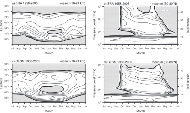
The quasi-biennial oscillation (QBO) is the primary mode of variability of the equatorial mean wind in the stratosphere (∼16-50 km), which is characterized by downward propagating easterly and westerly wind regimes, with a variable period averaging approximately 28 months (Baldwin et al.,2001). The maximum amplitude is observed in the middle and lower tropical stratosphere, with the easterly phase having larger amplitudes compared to the westerly phase. Figure 1.8a shows the equatorial zonal wind anomalies from 1965 to 1991, from control simulation performed with CESM1(WACCM) (see Chapter2for detailed simulation description). QBO first appears in the upper stratosphere and then propagates downward to the lower stratosphere. In the upper stratosphere, the more chaotic zonal wind regime are observed with a period of approximately 6 months, which is mainly attributed to the Semi-Annual Oscillation (SAO). QBO is forced by the interaction of long-period, vertically propagating tropical atmospheric waves (e.g., gravity, inertia- gravity, Kelvin and mixed Rossby-gravity waves) with the zonal mean flow, including (Lindzen and Holton,1968). These waves transfer momentum in the stratosphere and initiate the downward migration of easterly and westerly wind regimes (Lindzen and Holton1968; Andrews et al.1987;

Baldwin et al.2001).

The dependence of the strength of stratospheric polar vortex on the phase of the tropical QBO was first proposed by Holton and Tan (1980). In the so-called Holton-Tan (HT) mechanism, the vortex remains in an undisturbed, colder state when the QBO is in its westerly phase, and favors a disturbed, warmer state during the east phase of the QBO (Holton and Tan1980,1982).

This is shown exemplarily in Fig1.8b for QBO west (WQBO) minus QBO east (EQBO) years in a 145-year control simulation performed with the CESM1(WACCM)¹. The mechanism for this is related to the shifting of the critical line toward the NH subtropics, followed by a poleward dis- placement of the planetary waveguide during the QBO east phase, which directs more waves to polar regions and decelerates the vortex through enhanced wave-mean flow interactions. In addition, the warmer and more disturbed polar vortex during the QBO east phase are often reflected with a higher frequency of sudden stratospheric warming (SSW) events (Labitzke,1982).

Lu et al. (2014) further elucidate the H-T mechanism by showing that a formation of a mid- latitude waveguide during the QBO east phase provides a favorable pathway for more upward

1Here the QBO is defined as the time series of the zonal wind, averaged between 2.8^oS and 2.8^oN and between 43 and 51 hPa. Values above 5 m/s represent the WQBO phase, values below -2.5 m/s the EQBO phase.

(25)

1.5. External Forcing Factors Influencing Stratospheric Variability 15

FIGURE 1.8: (a) The time evolution of equatorial winds averaged between 2.8^oS to 2.8^oN from CESM1(WACCM) 1965 -1991. The seasonal cycle was removed from the data. Contour Interval is 5 m/s.

(b) Differences in zonal mean wind (m/s) between westerly and easterly QBO phase in DJF, from control simulation performed with CESM1(WACCM), 1955-2099. Colours indicate statistical significance (>95%) based on a two-tailedttest. Contour interval is 2 m/s.

(35-50^oN, 30-200 hPa) and northward (35-60^oN, 20-5 hPa) propagating planetary waves, which eventually dissipate and break in the high-latitude upper to middle stratosphere. However, some studies (e.g., Naoe and Shibata2010; Garfinkel et al.2012) argued that the QBO-induced secondary meridional circulation is more important than the subtropical critical line for the polar QBO signals during the east phase of the QBO. The secondary QBO circulation acts as a barrier for planetary wave propagation in the middle to upper stratosphere during the easterly phase, resulting in enhanced wave convergence in the polar stratosphere and therefore, a more disturbed polar vortex. Even though the evidence is inconclusive as to which mechanism dominates the QBO-vortex interaction, both the aforementioned mechanisms contribute to the breakdown of the polar vortex.

The direct impact of the QBO on the tropical and subtropical troposphere involve a modification of temperature and vertical wind shear along the tropopause (e.g., Gray et al. 1992; Ho

(26)

16 Chapter 1. General Introduction et al.2009; Yoo and Son2016). In the high latitudes, the QBO impact on the polar stratosphere is mostly indirect, which involves a modulation of the mid latitude planetary wave activity and the subsequent wave-mean flow interaction in the polar stratosphere (e.g., Holton and Tan1982;

Garfinkel et al.2012). The QBO signal in the NH high latitudes can propagate downward to the surface through the NAM, with a lag of approximately a few weeks (e.g., Baldwin and Dunkerton, 1999; Coughlin and Tung, 2001). Connections have also been found between QBO and regional winter surface climate (e.g., Marshall and Scaife2009).

In this thesis, the importance of the QBO signal for the stratosphere-troposphere coupling mechanism via DWC will be discussed in Chapter2. A detailed description of more aspects of the QBO can also be found in Chapter2.

1.5.2 Sea Surface Temperatures

Sea surface temperature (SST) is the interference between the ocean and the overlying atmosphere.

As such, it controls the exchange of heat and gases between the atmosphere and ocean. SST anomalies can affect the atmosphere through altering the flux of latent and sensible heat from the ocean, and thus providing anomalous heating patterns. Like the QBO, SSTs play a significant role in driving stratospheric variability at high latitudes. For example, Figure1.9shows the observed upper tropospheric height anomalies during the Northern Hemisphere winter during an El Niño-Southern Oscillation (ENSO) event in the tropical Pacific. The patterns resemble the Pacific North American (PNA) pattern of middle and upper tropospheric height anomalies. The anomaly pattern strongly suggests a train of stationary Rossby waves that emanates from the equatorial source region and follows a great circular path, as predicted by barotropic Rossby wave theory (Horel and Wallace, 1981). In this manner, tropical SST anomalies may generate low-frequency variability in the extratropics.

Several mechanisms have been proposed to explain the impact of SSTs on the variability of the polar stratosphere (e.g., Loon and Labitzke1987; Manzini et al.2006; Calvo et al.2009; Hur- witz et al. 2012; Li and Lau 2013; Omrani et al. 2014). For example, Loon and Labitzke (1987) firstly presented how tropical SSTs can influence the stratospheric polar vortex during the warm phase of ENSO (i.e., El Niño). They showed that warm ENSO events are associated with increased frequency of SSWs, and therefore a warmer and more disturbed polar vortex. This was further confirmed by some general circulation model (GCM) studies (e.g., Hamilton1993; Manzini et al.

2006) showing that the warmings observed during El Niño years are associated with the ampli- fication of upward planetary wave convergence. More recently, using the global coupled climate model GFDL-CM3, Li and Lau (2013) showed that enhancement or attenuation of the amplitudes of zonal wavenumbers 1 and 2 during ENSO events modulates the frequency of occurrence of stratospheric polar vortex anomalies. By combining ENSO-QBO effects on the vortex state, Calvo et al. (2009) showed that weak and warm polar vortex occur during warm ENSO in the late winter during both QBO phases. In addition to ENSO, other mechanisms including large scale North Atlantic temperature (Omrani et al., 2014; Keenlyside and Omrani, 2014; Omrani et al., 2015),

(27)

1.5. External Forcing Factors Influencing Stratospheric Variability 17

FIGURE1.9: Global pattern of middle and upper tropospheric geopotential height anomalies (solid) for NH winter during an ENSO event in the tropical Pacific. The anomaly pattern propagates along a great circle path with an eastward component of group velocity as predicted by stationary Rossby wave theory (Horel and Wallace,1981). Arrows depict a 500-hPa streamline for the anomaly conditions. H and L designate anomalous highs and lows, respectively. Region of enhanced tropical precipitation is shown by shading.

Figure from Horel and Wallace (1981).

extra-tropical SST in the Pacific basin (Hurwitz et al.,2012) and sea-ice (Jaiser et al.,2013) are also important for stratospheric variability through ocean-atmosphere coupling mechanisms.

There is a growing body of literature, much of it very recent, showing the importance of SSTs in modifying storm track dynamics and enhancing the tropospheric response to stratospheric forcing.

This includes the response to the solar cycle (e.g., Thieblemont et al.2015; Scaife et al.2013, and ozone (Ogawa et al., 2015). While the exact dynamical mechanism by which SSTs enhance the tropospheric response needs further study, a possible relevant mechanism is the enhancement of storm tracks and their associated internal variability (the annular modes) in the presence of SST gradients or fronts (e.g., Nakamura et al.2008; Sampe et al.2013).

Since SST variability influences the tropospheric wave source and the polar vortex, the coupling to the ocean can therefore influence the strength of DWC between the stratosphere and troposphere. In this thesis, the impact of SST variability on DWC in the NH is investigated in detail in Chapter2.

1.5.3 Greenhouse Gases and Ozone Depleting Substances

Significant changes in concentrations of key radiative gases in the stratosphere are expected over the 21st century (ozone is expected to increase as the concentrations of ODS decrease back to 1960 levels, and GHGs are expected to continue to increase e.g., IPCC2013; WMO2014). Figure1.10 shows the simulated global column ozone from 1960-2100, carried out using CCM simulations during Validation Activity for the second round (CCMVal-2). The projection represents a mean across the different CCM simulations. It is shown that the continuing slow decline of ODSs, and

(28)

18 Chapter 1. General Introduction the expected further increase of CO2, will contribute to a recovery of stratospheric ozone (Fig1.10).

In the second half of the century, ozone columns may even exceed historical levels.

FIGURE1.10: Simulated and observed evolution of the near global total ozone column. Observations are annual mean anomalies averaged over all available ground- and satellite-based measurements (blue line).

Black line and gray range give multi-model mean and±2 standard deviations of simulated individual model annual mean anomalies for the CCMVal-2 simulations. Figure from WMO (2014).

The role of stratospheric ozone in driving recently observed SH circulation and climate changes over last three decades has been shown by a number of observation and model studies (e.g., Ar- blaster and Meehl2006; Karpechko et al.2008; Butler et al.2010; McLandress et al.2010; Polvani et al. 2011; Thompson et al. 2011). By comparing simulations with both ozone and GHG forcings to simulations with GHG forcing alone, Polvani et al. (2011) showed that ozone depletion has been the dominant driver of recently observed atmospheric circulation changes in the SH during summer, with the GHG increases only playing a secondary role. This conclusion is not based solely on this model result, but is substantiated by the large number of observational and modelling studies mentioned above.

Most studies on the impact of GHG and ODS on the polar stratosphere in the NH are mainly addressed in model studies using 21st century GHG and ODS emission scenarios. An early study by Shindell et al. (1998) showed a significant cooling (and strengthening) of the Arctic vortex in the future as GHGs increased, which leads to significant ozone depletion and formation of an Arctic ozone hole. However, more recent simulations with more sophisticated CCMs, which have a better representation of the dynamics and chemistry (and couplings between them), do not show a significant strengthening or formation of Arctic ozone holes during the 21st century (e.g., Austin and Butchart2003; Eyring et al.2007). The CCMs also predict a limited impact of increased GHGs on the Antarctic vortex during the 21st century. However, the same simulations all predict an increase in the tropical upwelling as GHGs increase, which has been attributed to changes in subtropical wave forcing (e.g., Garcia and Randel2008; Oman et al.2009).

(29)

1.6. Dynamical Coupling of the Stratosphere and Mesosphere 19 In terms of SSWs, a consensus regarding future changes in the frequency of SSWs could not be achieved due to the wide range of results, ranging from an increase in the frequency of MSWs in the future to a decrease (e.g., Charlton-Perez et al.2008; Bell et al.2010a; Mitchell et al. 2012;

Ayarzaguena et al. 2013). These discrepancies have also been found in different CCM simulations under the same future scenario (SPARC CCMVal,2010). A possible reason for these discrepancies might be related to the weak amplitude of future changes in the Arctic polar vortex due to the competition of different contributors (e.g., GHG and ODS), or the biases in reproducing the related processes (SPARC CCMVal,2010; Mitchell et al., 2012). More recently, Manzini et al.

(2014) showed that the majority of the Coupled Model Intercomparison Project Phase 5 (CMIP5) models tends to predict future weakening of the winter stratospheric polar vortex under the extreme emission Representative Concentration Pathways (RCP8.5) scenario. Previous studies have proposed that there are at least two possible mechanisms that elucidate future weakening of the polar vortex associated with increased GHG emissions: (1) it is related to changes in the stratospheric meridional overturning circulation due to changes in the tropospheric wave source (e.g., Butchart and Scaife 2001; Garcia and Randel 2008; Wang and Kushner2011); (2) changes in the location of critical layers within the subtropical lower stratosphere (e.g., Eichelberger and Hartmann2005; McLandress and Shepherd2009; Shepherd and McLandress2011).

This thesis examines how DWC variability between the stratosphere and troposphere, particularly their seasonality, will change in the future, and how different anthropogenic forcing factors individually impact the occurrence of these events (Chapter4). In addition, the relative roles of GHG and ODS in controlling the vertical coupling of the stratosphere-MLT system in the SH during the Antarctic ozone hole period will be also investigated in this thesis (Chapter5).

1.6 Dynamical Coupling of the Stratosphere and Mesosphere

The dynamical linkage between the stratosphere and mesosphere has been discussed with respect to the upward influence of small-scale gravity waves, in recognition of the fact that the source of upward-propagating gravity waves is in the lower atmosphere (e.g., Holton1983; Andrews et al.1987; Fritts and Vadas2008). Gravity waves can be generated by mountain barriers, deep convection, and shear instability of the mean flow. Vertically propagating gravity waves from the troposphere into the mesosphere are strongly dependent on the variation of background stratospheric winds (e.g., Holton1983; Plumb2002). Figure1.11shows an approximate total non-resolved (gravity) wave drag in the middle atmosphere calculated as a residual of the transformed Eulerian mean (TEM) zonal momentum equation (see for details in Chapter5). It is shown that the underlying stratospheric winds selectively filter upward propagating gravity waves, leaving only a net westerly drag in the summer mesosphere and a net easterly drag in the winter hemisphere (Holton1983, Fig1.11). The breaking of gravity waves in the mesosphere deposits angular momentum and energy on the mean flow, which therefore affect the residual-mean circulation and temperatures there (e.g., Manzini et al.2003; Yamashita et al.2010; Li and Lau2013).

(30)

FIGURE1.11: Total non-resolved wave drag computed as a residual of the TEM zonal momentum equation averaged over (a) December to February (DJF) and (b) June to August (JJA), from the 145-yr control simulation performed with CESM1(WACCM). Contour lines indicate the zonal mean wind climatology. Contour interval is 10 m/s. See detailed formulation in Chapter5.

The dynamical coupling of the stratosphere and mesosphere can be examined during SSW events (e.g., Walterscheid et al.2000; Liu and Roble2002; Cho et al.2004; Limpasuvan et al.2012).

Previous studies showed that the polar mesospheric temperature and wind during NH winter can change significantly during SSW events (e.g., Walterscheid et al. 2000; Liu and Roble 2002), characterized by mesospheric cooling, deceleration or reversal of the mesospheric zonal wind, and change of the residual circulation. In the SH, the mesospheric cooling and mesospheric jet reversal (Dowdy et al., 2004) were observed above Antarctica prior to the unprecedented major SSW in 2002 (Baldwin et al.,2003). These changes in the mesosphere are likely caused by changes in gravity wave forcing (e.g., Liu and Roble2002). In addition, the associated changes in the polar mesospheric zonal wind can also affect the wave growth and propagation in the lower atmosphere (e.g., Tung and Lindzen1979; Liu and Roble2002; Coughlin and Tung2005), which in turn affect the course of the SSW event.

Another evidence of the stratosphere-mesospheric coupling can be examined during the Antarc- tic ozone hole period (e.g., Smith et al.2010; Lossow et al.2012; Lubis et al.2016a). The primary mechanism for this is changes in the propagation of gravity waves due to the strengthening of the stratospheric winds induced by the ozone hole (Smith et al., 2010; Lossow et al., 2012; Lu- bis et al.,2016a). The ozone hole leads to trends in the lower stratosphere temperature and winds during late spring to early summer. The trend in the stratospheric wind, as simulated in the Whole Atmosphere Chemistry Climate Model (WACCM), affected the propagation of gravity waves into

(31)

1.7. The Advantages of Climate Models 21 the mesosphere (Smith et al., 2010). As a result, the model simulations showed a weakening of polar summer mesosphere and a warming summer mesopause due to change in gravity wave interaction. This proposed mechanism by Smith et al. (2010) was later confirmed by other CCM studies (e.g., Lossow et al.2012; Lubis et al.2016a) and was verified by observation (Venkateswara Rao et al.,2015). However, until now an explicit interplay between planetary and gravity waves in explaining the enhanced anomalous polar descent from the mesosphere during the Antarctic ozone hole period remains unclear. In addition, it is still not well understood how large the radiative effects from increased GHGs affect the polar MLT response to the ozone hole. The results in this thesis reveal that a proper accounting of both dynamical and radiative effects is required in order to correctly attribute the causes of the polar stratosphere-MLT responses to the Antarctic ozone hole. These results are given in Chapter5.

1.7 The Advantages of Climate Models

Climate models are sophisticated numerical tools designed to simulate the interactions of the important drivers of climate, and to project the future state of the global climate system (IPCC, 2013). While progress in computer science in the past decades has been rapid, the capability of state-of-the-art climate models to realistically simulate the complex interactions of processes in the Earth’s climate system has increased (Reichler and Kim,2008). State-of-the-art GCMs are not only run in a stand-alone version with many prescribed input datasets, but are also used as a part of Earth System Models, which includes the interactive simulation of the ocean, land surface, and also recently, chemical processes. Figure1.12shows the development of climate models over the last 35 years, and shows how the different components were coupled into comprehensive climate models over time. The first climate model was initiated in the mid 1970s (Fig1.12), when scientists began to measure and interpret increasing atmospheric CO2. As satellite technology developed, the representations of Earth system processes in climate models are much more extensive and improved, particularly for the radiation and the aerosol cloud interactions and for the treatment of the cryosphere. The representation of the carbon cycle was added to a larger number of models and has been improved since the fourth assessment report (AR4) of the IPCC. A high-resolution stratosphere with interactive chemistry and an enhanced representation of nitrogen effects on the carbon cycle have now been included in many climate models in AR5 (IPCC,2013).

The Coupled Model Intercomparison Project 5 (CMIP5) [e.g., Taylor et al.2011], an important input to the AR5, has produced a multi-model data set that is designed to advance our understanding of climate variability and climate change. Building on previous CMIP efforts, CMIP5 includes long-term simulations of 20th century climate and projections for the 21st century and beyond. Previous studies have shown CMIP5 models with a comparably higher lid height or boundary ("high top") have a better representation of the stratosphere and its coupling to the troposphere (e.g., Manzini et al.2014), while CMIP5 models with a lower lid height ("low top") tend to