Factors for the Coupling Between the Stratosphere and the Troposphere
Dissertation
zur Erlangung des Doktorgrades
der Mathematisch-Naturwissenschaftlichen Fakult¨ at der Christian-Albrechts-Universit¨ at zu Kiel
vorgelegt von
Felicitas K. Hansen
Kiel, 2015
Tag der m¨ undlichen Pr¨ ufung: 11.05.2015
Zum Druck genehmigt: 11.05.2015
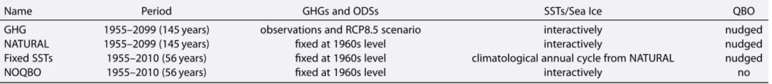
and the troposphere, and how this coupling is influenced by different natural and anthropogenic fac- tors. A unique set of four long-term sensitivity experiments is designed to examine the importance of the Quasi-Biennial Oscillation (QBO) of equatorial stratospheric winds, modes of sea surface temperature (SST) variability like the El Ni˜no Southern Oscillation (ENSO), anthropogenic green- house gases (GHGs) and ozone depleting substances (ODSs), for stratosphere-troposphere coupling.
The model experiments are performed with NCAR’s CESM model with the chemistry-climate model WACCM as its atmospheric component. The number and the length of the simulations performed here, given that the model includes both an interactive ocean and an interactive chemistry module and reaches up to the thermosphere, are exceptional.
Special emphasis is placed on major Stratospheric Sudden Warmings (SSWs) in the Northern hemisphere which are a prominent example of stratosphere-troposphere coupling and which can affect surface weather and climate. It is shown that the QBO strengthens the climatological stratospheric polar night jet (PNJ) and significantly reduces the major SSW frequency by reducing the propagation of planetary waves into the PNJ region. Variability in SSTs weakens the PNJ and significantly increases the major SSW frequency by enhancing planetary wave forcing. Extreme climate change conditions determine the prewarming phase of major SSWs. SST variability is needed to reproduce the observed tropospheric negative Northern Annular Mode pattern after major SSWs.
Further testing the sensitivity of WACCM experiments to the width of the QBO relaxation along the equator leads to a new contribution to the famous Holton-Tan mechanism in stratospheric dynamics and chemistry. The Holton-Tan mechanism, i.e., stronger zonal mean winds during QBO west phases (QBOW) in the PNJ region, is enhanced for a wider compared to a narrower QBO relaxation. The results suggest that at least two processes are involved in transmitting the equatorial QBO signal into the polar stratosphere: first, an effect of the zero wind line in the lower stratosphere which is shifted depending on the phase of the QBO, and second, the effect of the secondary QBO circulation in the middle to upper stratosphere. Both processes affect the direction of planetary wave propagation so that these waves disturb the stratospheric polar vortex more during QBO east phases (QBOE).
The first study which investigates a combined QBO-ENSO influence on the troposphere shows that large differences occur between the North Pacific and North Atlantic. The stratospheric equa- torial QBO anomalies extend down to the troposphere over the North Pacific during boreal winter, but only during La Ni˜na (not El Ni˜no) events. The conditions for the genesis and intensification of synoptic-scale waves are improved during QBOW compared to QBOE conditions by linear QBO- ENSO interactions. In the North Atlantic, the non-linear interaction of QBOW with La Ni˜na (QBOE with El Ni˜no) results in a positive (negative) North Atlantic Oscillation pattern.
This thesis presents an improved understanding of the physical mechanisms that couple the stratosphere and the troposphere, which has the potential to improve tropospheric weather forecast- ing skill and moreover highlights the importance of the stratosphere for understanding and modeling
und Troposph¨are und wie diese Kopplung von verschiedenen nat¨urlichen und anthropogenen Fak- toren beeinflusst wird. Um die Bedeutung der quasi-zweij¨ahrigen Schwingung des Windes in der
¨
aquatorialen Stratosph¨are (engl. Quasi-Biennial Oscillation, QBO), von Variabilit¨aten der Meeres- oberfl¨achentemperatur (engl. sea surface temperature, SST) wie z.B. die El Ni˜no Southern Oscil- lation (ENSO), von anthropogenen Treibhausgasen und von ozonzerst¨orenden Substanzen f¨ur die Stratosph¨aren-Troposph¨aren-Kopplung zu untersuchen, wurde ein einzigartiges Set aus vier langen Sensitivit¨atsexperimenten entworfen. Die Modellexperimente wurden mit NCAR’s CESM Modell durchgef¨uhrt, welches das Klima-Chemie-Modell WACCM als atmosph¨arische Komponente beinhal- tet. Die Anzahl und die L¨ange der Simulationen mit solch einem komplexen Modellsystem, das sowohl einen interaktiven Ozean als auch ein interaktives Chemie-Modul enth¨alt und das bis in die Thermosph¨are hinaufreicht, sind außergew¨ohnlich.
Ein spezieller Fokus dieser Arbeit lag auf der Untersuchung von großen pl¨otzlichen Stratosph¨aren- erw¨armungen in der Nordhemisph¨are, da diese ein bekanntes Beispiel f¨ur Stratosph¨aren-Tropo- sph¨aren-Kopplung darstellen und sogar das Wetter und Klima an der Erdoberfl¨ache beeinflussen.
Die Ergebnisse dieser Arbeit zeigen, dass die Pr¨asenz der QBO den klimatologischen Polarnacht- strahlstrom in der Winter-Stratosph¨are verst¨arkt und die Anzahl von großen Stratosph¨arenerw¨ar- mungen signifikant dadurch verringert, dass die Ausbreitung von planetarischen Wellen in die Polar- nachtstrahlstrom-Region reduziert wird. Variable SSTs schw¨achen den Polarnachtstrahlstrom und erh¨ohen die Frequenz von großen Stratosph¨arenerw¨armungen dadurch, dass die Wellenausbreitung in die Polarnachtstrahlstrom-Region verst¨arkt wird. Extreme Klimawandel-Bedingungen haben einen Einfluss auf die dynamische Entwicklung in den Wochen vor den großen Stratosph¨arenerw¨armungen.
Variable SSTs werden ben¨otigt, um das beobachtete negative Signal der Nordatlantischen Oszillation in der Troposph¨are im Anschluss an große Stratosph¨arenerw¨armungen richtig zu reproduzieren.
Weitere Analysen bez¨uglich der Breite der QBO-Relaxierung am ¨Aquator konnten zu einem besseren Verst¨andnis des bekannten Holton-Tan-Mechanismus’ beitragen. In dieser Arbeit wurde gezeigt, dass der Holton-Tan-Mechanismus, der st¨arkere Zonalwinde in der polaren Stratosph¨are w¨ahrend QBO-West-Phasen bewirkt, verst¨arkt ist, wenn eine breitere QBO-Relaxierung gew¨ahlt wird. Zwei Prozesse scheinen haupts¨achlich f¨ur die ¨Ubermittlung des ¨aquatorialen QBO-Signals in die polare Stratosph¨are verantwortlich zu sein: zum einen der Effekt der Nullwindlinie in der un- teren Stratosph¨are der niederen Breiten, die abh¨angig von der QBO-Phase verschoben wird, und zum anderen der Effekt der sekund¨aren QBO-Zirkulation in der mittleren und oberen Stratosph¨are der mittleren Breiten. Beide Effekte bewirken eine ¨Anderung der Ausbreitungsrichtung von plane- tarischen Wellen, sodass diese w¨ahrend der QBO-Ost-Phase in Richtung des Polarnachtstrahlstromes gelenkt werden und den Polarwirbel st¨oren und abschw¨achen.
In der ersten Studie, die den kombinierten QBO-ENSO-Einfluss auf die Troposph¨are untersucht, konnte gezeigt werden, dass bei diesem Einfluss große Unterschiede zwischen dem Nord-Pazifik und dem Nord-Atlantik auftreten. Die QBO-Anomalien breiten sich aus der ¨aquatorialen Stratosph¨are bis
w¨ahrend der QBO-Ost-Phasen. Im Nord-Atlantik sorgen nicht-lineare Wechselwirkungen zwischen QBO-West-Phasen und La Ni˜na-Bedingungen (QBO-Ost-Phasen und El Ni˜no-Bedingungen) f¨ur die Entstehung eines positiven (negativen) Musters der Nordatlantischen Oszillation.
Diese Arbeit tr¨agt zu einem besseren Verst¨andnisses der physikalischen Prozesse von Stratosph¨aren- Troposph¨aren-Kopplung bei. Dies birgt Potenzial zur Verbesserung der G¨ute von troposph¨arischen Wettervorhersagen. Die Ergebnisse dieser Arbeit betonen auch die Relevanz der Stratosph¨are f¨ur die Dynamik in der Troposph¨are.
1 Introduction 3
1.1 Coupling between Stratosphere and Troposphere . . . 3
1.1.1 Stratospheric Sudden Warmings (SSWs) . . . 4
1.2 Factors of natural climate variability . . . 5
1.2.1 The Quasi-Biennial Oscillation . . . 6
1.2.2 Sea Surface Temperatures . . . 7
1.2.3 Other natural factors. . . 8
1.2.4 Impact on NH zonal mean temperature . . . 10
1.3 The need for climate models. . . 15
1.3.1 A special problem: the QBO in climate models . . . 15
1.4 Scientific questions of this thesis . . . 16
2 The influence of natural and anthropogenic factors on Major Stratospheric Sudden Warmings 19 3 Sensitivity of stratospheric dynamics and chemistry to QBO nudging width in the chemistry-climate model WACCM 41 4 Tropospheric QBO-ENSO interactions and differences between Atlantic and Pa- cific 55 5 Summary 97 5.1 Outlook . . . 100
Bibliography 103 Own Publications 111 Appendix 113 A.1 Multiple Linear Regression (MLR) Analysis . . . 113
Danksagung 115
The two lowermost layers in the Earth’s atmosphere - the troposphere and the stratosphere - are not strictly separated but vertically coupled via various dynamical, chemical and radiative processes. Of these processes, the dynamical coupling deserves special consideration given that large stratospheric anomalies can propagate down into the troposphere and even have an effect on the surface. Thus, detailed understanding of dynamical stratosphere-troposphere coupling contains large potential to enhance skill for predictions of tropospheric weather and climate.
The coupling between the stratosphere and the troposphere can be influenced by those factors which determine atmospheric variability. The appearance of this modulation and the underlying physical mechanisms are far from being fully understood. However, it is crucial to separate and quantify the contributions from natural and anthropogenic factors for these mechanisms, e.g., in order to reli- ably estimate the anthropogenic contribution to the recent tropospheric warming and stratospheric cooling trend, and therefore improve projections of the future climate.
The goal of this thesis is to provide qualitative and quantitative estimates about the impact of dif- ferent natural and anthropogenic factors on stratosphere-troposphere coupling. Underlying physical mechanisms for this coupling will be investigated.
1.1 Coupling between Stratosphere and Troposphere
Several theories exist on the mechanisms for the dynamical coupling between the stratosphere and the troposphere. Haynes et al. [1991] proposed the so-called ”downward control” principle. It suggests that zonal forces which occur due to the dissipation of Rossby and gravity waves in the stratosphere induce a secondary circulation which extends down to the troposphere. Another idea involves the adjustment of the tropospheric flow to stratospheric potential vorticity anomalies [Hartley et al., 1998; Black, 2002; Black and McDaniel, 2004]. Other studies indicate a potential role of synoptic eddies for the downward coupling of stratospheric anomalies and the persistence of the signal in the troposphere [Kushner and Polvani,2004;Song and Robinson, 2004;Simpson et al.,2009;Kunz and Greatbatch, 2013; Domeisen et al., 2013]. Kunz and Greatbatch [2013] report that quasi- geostrophic adjustment of the troposphere to stratospheric wave drag initiates a surface response to the stratospheric anomalies, and that this surface response is delayed up to several weeks with respect to the stratospheric signal due to eddy feedback processes.
considered. Planetary waves are generated in the troposphere by orography and land-sea contrasts.
These waves propagate upward into the stratosphere where they either dissipate or are reflected downward to impact the troposphere again, e.g., through feedback processes with synoptic-scale waves.
Planetary waves can propagate only in a certain range of westerly wind regimes [Charney and Drazin, 1961]. When they dissipate in the stratosphere, they interact with the zonal-mean flow and accelerate or decelerate the prevailing background winds; the resulting anomalies can propagate downward. This process has been shown to be of potential importance for seasonal prediction and weather forecasts of tropospheric NH winter weather [Baldwin and Dunkerton, 2001; Thompson et al., 2002; Baldwin et al., 2003; Mitchell et al., 2013; Sigmond et al., 2013]. Several indices are used to assess this zonal-mean coupling. Many of them are based on the annular modes in both hemispheres (NAM and SAM, respectively), which are commonly defined as the leading empirical orthogonal functions (EOFs) of monthly-mean hemispheric geopotential height fields [Baldwin and Thompson, 2009]. Others use, e.g., the zonal mean wind at a certain latitude and height, or parameters at the polar cap. In a comparison of these indices, Baldwin and Thompson [2009]
highlight the advantages of a methodology based on EOFs of daily zonally-averaged geopotential.
According to their results, the daily evolution of stratosphere-troposphere coupling is seen most clearly with this method, it is robust, easy to apply to climate model output in zonal-mean form and computationally less expensive than other methods.
Especially weak and strong stratospheric events, defined via the various indices, have the potential to propagate downward and affect the troposphere. A prominent example of such an extreme event in the stratosphere is the weak polar vortex event, a so-called Stratospheric Sudden Warming (SSW;
see below).
The process of planetary waves being reflected in the stratosphere to affect the troposphere again is called downward wave coupling. It represents another important source of stratosphere-troposphere coupling. Fundamental research on this topic has been mainly done by N. Harnik, J. Perlwitz and T. Shaw [e.g., Harnik and Lindzen, 2001; Perlwitz and Harnik, 2003, 2004; Harnik, 2009; Shaw et al., 2010]. They found that the occurrence of downward wave coupling is tied to a so-called
”bounded wave geometry”, meaning a well-defined high-latitude meridional waveguide in the lower stratosphere that is bounded above by a vertical reflecting surface.
Recent dynamical metrics of stratosphere-troposphere coupling are based on extreme stratospheric planetary-scale wave heat flux events [Shaw et al., 2014], tropospheric blockings [Davini et al., 2014], or Mark Baldwins idea of a stratospheric ”plunger” (not published yet), meaning anomalies of potential vorticity affecting the tropopause height and thereby stratosphere-troposphere coupling.
1.1.1 Stratospheric Sudden Warmings (SSWs)
Planetary waves propagate upward from the troposphere into the stratosphere only in (not too
during summer when easterly winds are prevailing. By the interaction of planetary waves with the zonal mean flow, the winter stratospheric polar vortex can be disrupted in its zonal symmetry [Matsuno, 1971]. It might then be displaced from the pole or split into two vortices, whereupon both processes lead to a fast (within a few days) and strong (up to several tens of ◦C) increase in temperatures in the polar stratosphere. If this temperature increase is accompanied by a reversal of the zonal mean zonal wind at 60◦N on the 10hPa level from westerly to easterly, the World Meteorological Organization (WMO; see Labitzke and Naujokat [2000]) calls this event a major Stratospheric Sudden Warming (SSW). A major SSW is observed about every two years [Erlebach et al., 1996; Labitzke and Naujokat, 2000; Charlton and Polvani, 2007]. More details about major warmings and how they are influenced by different natural and anthropogenic factors can be found in Chapter 2.
At the end of each winter, the stratospheric winds switch from westerly to the easterly summer circulation; this event is called final warming. A major SSW occurring during this transition period without a circulation change back to the winter westerlies is called major final warming accordingly.
When the polar temperature increases but the circulation at 10hPa does not reverse, the event is defined as a minor warming. Theoretically, major, minor and final warmings can occur in both hemispheres. However, since less waves are generated in the Southern hemisphere due to less land masses and hence dynamics which are very different from the NH, only one major warming occurred until now in the Southern Hemisphere (SH) since the beginning of detection in the 1940s [Kr¨uger et al.,2005]. There exists no SH counterpart of the so-called Canadian warmings which happen in the NH in early winter.
Large stratospheric anomalies like those occurring during major SSWs have the potential to descend down into the troposphere and thus even affect surface weather and climate [Julian and Labitzke, 1965; Quiroz, 1977; Baldwin and Dunkerton, 2001; Thompson et al., 2002; Mitchell et al., 2013;
Hitchcock and Simpson, 2014], and even the ocean [e.g., Reichler et al., 2012; O’Callaghan et al., 2014]. The resulting surface pattern strongly projects on the negative phase of the North Atlantic Oscillation (NAO) or the Arctic Oscillation (AO) [Baldwin and Dunkerton, 2001; Charlton and Polvani, 2007]. Examples of the surface influence of SSWs are an effect on North American, European [Mitchell et al., 2013] or northern Russia [Sigmond et al., 2013] surface temperatures, eastern Canada and North Atlantic precipitation [Sigmond et al., 2013], or 500hPa geopotential height over Europe [Domeisen et al., 2015].
1.2 Factors of natural climate variability
From the effect of stratospheric anomalies on tropospheric weather and climate it follows that the coupling mechanisms described above can be used to improve tropospheric weather forecasts and seasonal predictions for different latitudes and regions [Baldwin and Dunkerton, 2001; Thompson
mandatory to gain detailed understanding about the processes underlying this coupling, and of potential influencing factors. This thesis wants to contribute to this gain of understanding (and at the end to the enhancement of tropospheric prediction skill) by investigating the importance of different so-called ”anthropogenic” and ”natural” factors for stratosphere-troposphere coupling.
The factors which can be assumed to influence stratosphere-troposphere coupling are the factors which determine the variability of each of the two layers separately. Some of these factors, namely greenhouse gases (the most prominent example of them is carbon dioxide,CO2) and ozone-depleting substances, have reached unsightly popularity in the last decades, as they have been shown to be responsible for the recent warming trend in global tropospheric temperatures and the accompanying cooling in the stratosphere (see assessment reports (AR) of the Intergovernmental Panel on Climate Change (IPCC), e.g. IPCC [2014]). The decline of the stratospheric ozone layer as well as changes in the ozone hole which forms over Antarctica each Southern hemisphere (SH) spring have been the focus of many chemistry studies. These studies agree that for the involved ozone depletion processes, catalytic chemistry including man-made chlorofluorocarbons are responsible [Solomon, 1999]. As GHGs and ODSs are produced and emitted due to human behavior, these factors are called
”anthropogenic”. Their counterpart are the so-called ”natural” factors, causing natural or internal climate variability. Natural factors are, e.g., internal factors like the Quasi-Biennial Oscillation (QBO) of equatorial stratospheric winds, variations in sea surface temperatures (SSTs), volcanic eruptions, or external factors like variations in solar radiation. These natural factors and their importance for tropospheric and stratospheric variability shall be briefly introduced in the following. More detailed descriptions, especially of the QBO and SST variability patterns, can be found in the following chapters.
1.2.1 The Quasi-Biennial Oscillation
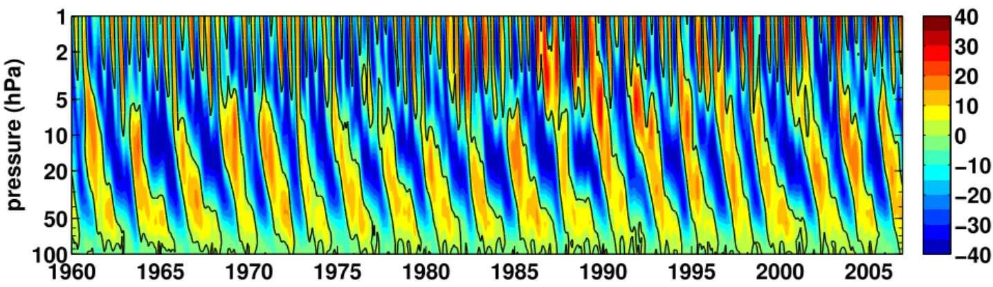
The QBO is the dominant natural variability mode in the equatorial stratosphere [Baldwin et al., 2001]. It is mainly driven by upward propagating tropical atmospheric waves like gravity, inertia- gravity, Kelvin and Rossby-gravity waves. These waves, which are smaller-scale compared to the previously introduced planetary waves, transfer momentum in the stratosphere and initiate the down- ward propagation of easterly and westerly wind regimes [Lindzen and Holton, 1968; Andrews and McIntyre,1976;Baldwin et al.,2001] as can be seen in Figure1.1. The wind regimes alternate with an average period of about 28 months. The amplitude of the wind regimes is asymmetric with a maximum of around +20 m/s in the westerly and -30 m/s in the easterly phase. By influencing the propagation of mid-latitude planetary waves and their interaction with the mean flow, the tropical QBO affects the mean state and variability in the extra-tropical and even polar stratosphere [Holton and Tan, 1980, 1982; Anstey and Shepherd, 2014]. In the latter, the stratospheric polar winter vortex is on average colder and less disturbed in QBO west phase winters, while it tends to be warmer and hence more disturbed in winters of dominating easterly QBO phase [Holton and Tan,
pressure (hPa)
1960 1965 1970 1975 1980 1985 1990 1995 2000 2005 1
2 5 10 20 50
100 −40
−30
−20
−10 0 10 20 30 40
Figure 1.1: Zonal mean zonal wind (m/s) in the equatorial stratosphere, averaged between 2.8◦S and 2.8◦N. Contour interval 5 m/s; the black contour indicates the zero wind line. From the extended ERA40 data set (see Chapter 3).
line depending on the QBO phase, which hinders or allows planetary waves to propagate into the tropical stratosphere. However, more recent studies [Naoe and Shibata,2010;Garfinkel et al.,2012]
suggest that the underlying mechanism is more a combination of this effect with another effect in the mid-latitude stratosphere which includes the QBO secondary meridional circulation. In the mid-latitude stratosphere, a ”barrier” for planetary waves is created depending on the QBO phase, leading to a convergence of these waves in the polar vortex region and hence a more disturbed vortex during QBOE. In Chapter 3 the importance of these two mechanisms for the QBO signal in the polar stratosphere will be addressed.
A detailed description of many more aspects of the QBO can also be found in Chapter 3.
Although the QBO is primarily a stratospheric phenomenon, there are at least two ways in which it can affect the troposphere: 1) directly in the tropics and subtropics by modifying, e.g., temper- ature and vertical wind shear along the tropopause and hence stratosphere-troposphere exchange [e.g., Gray et al., 1992], or 2) indirectly through its modulation of the stratospheric polar vortex which can be seen at the surface with a lag of 2–3 weeks [e.g., Baldwin and Dunkerton, 1999].
The tropospheric impact of the QBO then occurs, e.g., as an influence on European winter surface climate [Marshall and Scaife, 2009], as a modulation of the tropospheric subtropical jet [Garfinkel and Hartmann, 2011a,b] or as a modulation of tropical cyclone tracks [Ho et al., 2009] and their frequency [e.g., Shapiro, 1989].
1.2.2 Sea Surface Temperatures
Variations in SSTs also have a strong impact on the variability not only in the lower, but also in the middle to upper atmosphere [e.g.,Sassi et al.,2004]. The dominant mode of SST variability between 60◦S and N is the oceanic component of the El Ni˜no-Southern Oscillation (ENSO) [Trenberth,1997].
ENSO is a seesaw between warm and cold SST anomalies in the equatorial Pacific with consequences
anomalously warm in the tropical Pacific ocean; during a cold ENSO phase (La Ni˜na), SSTs are anomalously cold in this region. The coupled atmospheric component of ENSO, the Southern Oscillation, appears as according anomalies in sea level pressure (SLP), wind or temperature around the equatorial Pacific, i.e., high SLP over the western tropical Pacific during El Ni˜no and low SLP in this region during La Ni˜na.
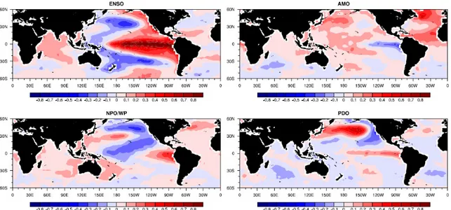
Aside from ENSO, other important large-scale SST variability patterns are the Atlantic Multidecadal Oscillation [Schlesinger and Ramankutty, 1994], the North Pacific Oscillation/West Pacific pattern [e.g.,Wallace and Gutzler,1981;Linkin and Nigam,2008], or the Pacific Decadal Oscillation [Mantua et al., 1997]. Figure 1.2 (from Blume [2012]) shows these variability patterns as the first four empirical orthogonal functions (EOFs) of observed monthly detrended SST anomalies.
Like the QBO, the effect of ENSO and other SST variability patterns is not restricted to their main occurrence regions. ENSO, although being a phenomenon of the tropical Pacific, has an effect on the global atmospheric circulation [e.g., Alexander et al., 2002]. There seems to be a tropospheric (via tropospheric teleconnections) and a stratospheric (mainly via SSWs) pathway of ENSO influencing the troposphere as recently summarized for reanalysis data byButler et al. [2014]. Via tropospheric teleconnection patterns like, e.g., the Pacific-North American pattern (PNA; Wallace and Gutzler [1981]), ENSO modulates the climate over North America. Its influence on the stratospheric polar vortex has been, e.g., confirmed in observations by van Loon and Labitzke [1987] and in model studies by Sassi et al.[2004];Manzini et al. [2006];Ayarzag¨uena et al. [2013]. During ENSO warm phases, the Aleutian low is deepened, and the planetary wave number 1 interferes positively with the climatological wave structure [Ineson and Scaife, 2009]. The resulting stronger wave forcing in turn leads to a weaker stratospheric polar vortex [Manzini et al., 2006; Ayarzag¨uena et al., 2013]
and more SSWs. Via this stratospheric pathway, ENSO affects the climate over the North Atlantic and Europe [Ineson and Scaife, 2009; Butler et al., 2014; Domeisen et al., 2015]. The resulting surface signal consists of a negative North Atlantic Oscillation (NAO) pattern, which leads, e.g., to cold late winters in Northern Europe during the ENSO warm phase [Ineson and Scaife, 2009].
Influencing the same regions, ENSO effects interact with the QBO. During El Ni˜no (La Ni˜na) phases, the amplitude of the QBO at the equator is weaker (stronger) and the period is shorter (longer) [Taguchi, 2010; Yuan et al., 2014]. In the stratospheric polar vortex region, El Ni˜no interacts non-linearly with the easterly QBO phase [Garfinkel and Hartmann, 2007; Calvo et al.,2009].
1.2.3 Other natural factors
Volcanic eruptions can influence climate variability by the injection of aerosols into the atmosphere.
Two processes are mainly involved in modulating global temperatures: first, the aerosol layer leads to an enhanced scattering of incoming solar radiation back to space, resulting in a cooling at the surface.
Second, by absorbing solar and terrestrial radiation, stratospheric temperatures increase [Robock, 2000]. Although stratospheric ozone depletion is enhanced after an eruption through heterogeneous
Figure 1.2: The first four empirical orthogonal functions (EOFs) of monthly observed detrended SST anomalies in Kelvin. Figure fromBlume [2012].
absorption and hence reduced radiative heating in the stratosphere, the net stratospheric effect is still heating. Because this stratospheric warming is stronger at low than at high latitudes, the equator-to- pole temperature gradient is enhanced which results in a stronger stratospheric polar vortex. A global influence of volcanic eruptions is more likely when the eruptions take place close to the equator:
by tropical convection, the injected aerosols are transported higher up into the atmosphere and are distributed globally with the Brewer-Dobson circulation, the meridional overturning circulation in the stratosphere [Brewer, 1949; Dobson, 1952]. Prominent examples of volcanic eruptions which were followed by a significant decrease in global surface temperature and an increase in stratospheric temperatures are the eruptions of Mt. Agung (1963), El Chich´on (1982), and Mt. Pinatubo (1991).
The stratospheric warming following such strong volcanic eruptions can last 1–2 years, the surface cooling even 1–3 years [Robock,2000].
Another non-negligible part of the variability in the climate system is generated by variations in solar irradiance (see review paper by Gray et al. [2010]). Strong variations in various atmospheric parameters like, e.g., ozone and temperatures occur with a period of 11 years [e.g., Haigh, 1994, 1996; Matthes et al., 2006; Frame and Gray, 2010] which is referred to as the 11-year solar cycle.
These variations are induced by a varying number of sunspots and faculae on the Sun’s surface.
Although the total solar irradiance changes only by about 0.07% between sunspot maximum and minimum [Gray et al., 2010], differences in the ultra-violet (UV) band of the spectrum can reach up to 8% [Lean et al., 1997]. This is of special importance for the ozone layer in the middle atmosphere where UV radiation is absorbed which in turn directly affects the radiation budget and hence atmospheric temperatures. Solar cycle induced changes in the meridional temperature gradient lead to changes in wind fields due to thermal wind balance. It occurs that the stratospheric
influence on the atmosphere interacts with effects of the QBO in such way that the Brewer-Dobson circulation is weakened during solar maximum conditions and the easterly phase of the QBO, and strengthened during solar maximum and the westerly QBO phase [Matthes et al.,2010].
1.2.4 Impact on NH zonal mean temperature
Both natural and anthropogenic factors have an influence on the whole atmosphere, albeit in differ- ent strength, depending, amongst others, on the altitude, the latitudinal region and the season. As the factors vary on different time scales and also interact with each other in a complex, non-linear way, it is difficult to separate their individual contributions and quantify their respective roles for the total variability. Some parts of the total variability might also be due to chaotic behavior [e.g., Holton and Mass,1976; Yoden, 1987a,b;Christiansen,2000;Badin and Domeisen, 2013].
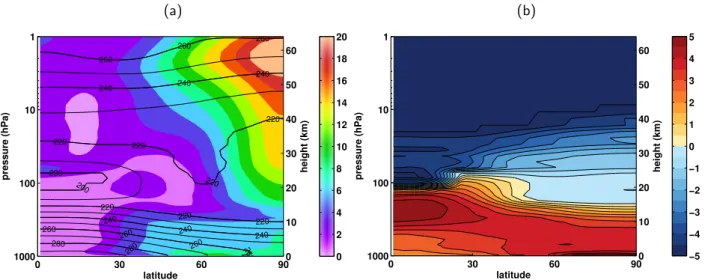
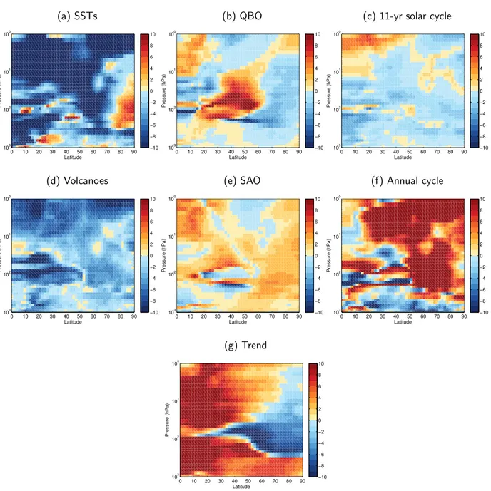
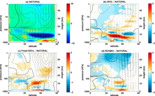
Figure1.3, left, shows zonally averaged NH tropospheric and stratospheric temperatures, and Figure 1.4 provides an estimate of the relative importance of the different factors for these temperatures.
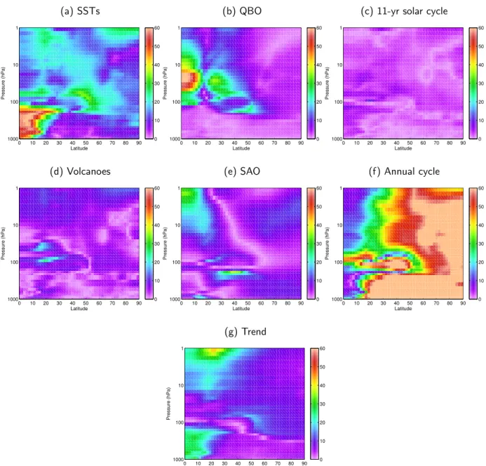
For Figure 1.4, the Linear Discriminant Analysis (LDA) is chosen and applied in a similar way as in Blume [2012]. The time series of zonal mean temperatures at each grid point in the zonal mean plane is modeled using a linear and stationary regression model where the time series of the different factors serve as forcing factors. The output of the LDA is a coefficient for each of the forcing factors, and from these coefficients the normalized impacts of the respective factors (which are shown in Figure1.4) for zonal mean temperatures can be computed (see Appendix A.1 for details). Data are taken from a simulation of the recent past (1955–1999) with the Community Earth System Model (CESM) (20th century part of the “GHG” simulation described in chapter 2).
Figure 1.4 shows that in the tropical troposphere, zonal mean temperature variability is dominated by variability in SSTs (maximum impact larger than 60%; Figure 1.4 a), originating mainly from ENSO (not shown)1. Higher up in the tropical stratosphere, the QBO becomes apparent as the dominant mode not only in zonal mean zonal wind but also in zonal mean temperatures (maximum impact larger than 60%; Figure 1.4 b). Its dominant influence reaches into the stratospheric sub- tropics, where a secondary QBO signal is induced in order to maintain thermal wind balance [Plumb and Bell, 1982]. In the upper tropical stratosphere, temperature variability is dominated by the stratospheric semi-annual oscillation (SAO; Figure 1.4 e) [Reed, 1966; Belmont et al., 1974; Gray and Pyle, 1986].
The largest impact - more than 70% - on extra-tropical NH zonal mean temperatures in both the troposphere and the stratosphere comes from variations due to the seasonal cycle (Figure 1.4 f).
The other factors are of secondary importance in the extra-tropics and play a role only locally, like, e.g., the SSTs in the mid-latitude lower stratosphere and high-latitude lower and upper stratosphere.
The impact of volcanic eruptions is strongest along the subtropical tropopause and in the upper
1As described in Appendix A.1, the LDA has been performed separately for the first four EOFs of daily detrended SST anomalies. The tropical tropospheric signal in Figure 1.4 (a) is dominated by the signal coming from the
stratosphere (Figure 1.4 d). However, with a maximum impact of around 25%, its relative impor- tance for NH zonal mean temperatures is small compared to the other factors. The same is true for the solar cycle (Figure 1.4 c). The influence of these factors on climate can be better seen using other methods, like in anomaly composites as done, e.g., in Kodera and Kuroda [2002]; Matthes et al. [2006]; Ineson et al. [2011]. The LDA applied here is not able to bare comparatively small signals which can be amplified by feedback processes; however, the method is sufficient to provide a estimate of the mean relative importance of the factors.
Compared to the other factors, the linear trend (Figure 1.4 g) is of special importance for the NH zonal mean temperature in the tropical troposphere (impact of ∼30%), the subtropical upper stratosphere (∼40%) and along the mid-latitude tropopause and stratosphere (10–20%) during the period 1955–1999.
The general picture presented here is consistent with the results from Mitchell et al. [2014] where multilinear regression techniques are applied to nine reanalysis data sets, and with other model stud- ies [e.g., Robock, 2000;Butchart et al.,2003;Giorgetta et al., 2006; Manzini et al.,2006].
From the method applied for Figure1.4, we can get a rough idea about the impact of the respective factors on NH global zonal mean temperature; however, the real impact is not zonally symmetric around the globe. Chapter 4of this thesis partly discusses this issue using the example of the QBO and its influence on different tropospheric sectors.
The impact of the different factors might change over time, e.g., due to changing atmospheric background states like the increase in GHGs since the industrial revolution which results in a tro- pospheric warming and stratospheric cooling trend (see Figure 1.3, right). Figure 1.5 shows how this impact change could look like for the period 2050–2099, using again the CESM ”GHG” sim- ulation, but now forced with the so-called Representative Concentration Pathways (RCP) Scenario 8.5. The RCP8.5 scenario is a strong GHG scenario which assumes an increase in radiative forcing of 8.5 W/m2 relative to preindustrial values. Following this scenario, the impact of the linear trend increases especially in the tropical and subtropical troposphere and stratosphere by 10%, and this increase mainly counterbalances the decreasing impact of SSTs in this region. The SSTs become increasingly important (+10%) in the polar lower stratosphere, and the impact of the QBO increases by∼10% in the mid-latitude lower stratosphere.
Altogether, it can be seen from this analysis that the natural and anthropogenic factors introduced before all have an impact on the stratosphere and the troposphere. However, as these two layers are not dynamically separated but vertically ”coupled”, the different factors also affect the stratosphere- troposphere coupling. Besides the seasonal cycle, the QBO and SSTs have the largest impact on NH zonal mean temperatures. This is why these two natural factors are chosen for this thesis for the following more detailed analysis on their importance for stratosphere-troposphere coupling, while the solar cycle, volcanic eruptions and the SAO are not further investigated here.
(a)
0 30 60 90
1
10
100
1000
latitude
pressure (hPa)
200 200
220
220 220
220 220
220
220
240
240 240
240 240
240
260 260 260
260
260
260
260
280 280
0 2 4 6 8 10 12 14 16 18 20
0 10 20 30 40 50 60
height (km)
(b)
latitude
pressure (hPa)
0 30 60 90
1
10
100
1000 −5
−4
−3
−2
−1 0 1 2 3 4 5
0 10 20 30 40 50 60
height (km)
Figure 1.3: Annual NH zonal mean temperatures. Mean (contours, contour interval 10K) and standard deviation (colours, contour interval 2 K) for the period 1955–1999 (a), and the difference between the 2050–2099 average and the 1955-1999 average (b; contour interval 0.5 K). Data from CESM ”GHG” simulation (see Chapter 2).
(a) SSTs
0 10 20 30 40 50 60 70 80 90
1
10
100
1000
Latitude
Pressure (hPa)
0 10 20 30 40 50 60
(b) QBO
0 10 20 30 40 50 60 70 80 90
1
10
100
1000
Latitude
Pressure (hPa)
0 10 20 30 40 50 60
(c) 11-yr solar cycle
0 10 20 30 40 50 60 70 80 90
1
10
100
1000
Latitude
Pressure (hPa)
0 10 20 30 40 50 60
(d) Volcanoes
0 10 20 30 40 50 60 70 80 90
1
10
100
1000
Latitude
Pressure (hPa)
0 10 20 30 40 50 60
(e) SAO
0 10 20 30 40 50 60 70 80 90
1
10
100
1000
Latitude
Pressure (hPa)
0 10 20 30 40 50 60
(f) Annual cycle
0 10 20 30 40 50 60 70 80 90
1
10
100
1000
Latitude
Pressure (hPa)
0 10 20 30 40 50 60
(g) Trend
0 10 20 30 40 50 60 70 80 90
1
10
100
1000
Latitude
Pressure (hPa)
0 10 20 30 40 50 60
Figure 1.4: Impact (in %) of different natural (1st and 2nd row) and anthropogenic (3rd row) factors on annual NH zonal mean temperatures during 1955–1999. For details about the computation of the impact and about the single factors see Appendix A.1. Data from CESM ”GHG” simulation (see Chapter2).
(a) SSTs
0 10 20 30 40 50 60 70 80 90
100
101
102
103
Latitude
Pressure (hPa)
−10
−8
−6
−4
−2 0 2 4 6 8 10
(b) QBO
0 10 20 30 40 50 60 70 80 90
100
101
102
103
Latitude
Pressure (hPa)
−10
−8
−6
−4
−2 0 2 4 6 8 10
(c) 11-yr solar cycle
0 10 20 30 40 50 60 70 80 90
100
101
102
103
Latitude
Pressure (hPa)
−10
−8
−6
−4
−2 0 2 4 6 8 10
(d) Volcanoes
0 10 20 30 40 50 60 70 80 90
100
101
102
103
Latitude
Pressure (hPa)
−10
−8
−6
−4
−2 0 2 4 6 8 10
(e) SAO
0 10 20 30 40 50 60 70 80 90
100
101
102
103
Latitude
Pressure (hPa)
−10
−8
−6
−4
−2 0 2 4 6 8 10
(f) Annual cycle
0 10 20 30 40 50 60 70 80 90
100
101
102
103
Latitude
Pressure (hPa)
−10
−8
−6
−4
−2 0 2 4 6 8 10
(g) Trend
0 10 20 30 40 50 60 70 80 90
100
101
102
103
Latitude
Pressure (hPa)
−10
−8
−6
−4
−2 0 2 4 6 8 10
Figure 1.5: Change of impact (in %) of different natural (1st and 2nd row) and anthropogenic (3rd row) factors on annual NH zonal mean temperatures during 2050–2099 relative to 1955-1999. Data from CESM ”GHG” simulation (see Chapter 2).
1.3 The need for climate models
When influencing the coupling between the stratosphere and the troposphere, the different natural and anthropogenic factors partly interact in a complex, non-linear way. This makes it complicated, if not impossible, to separate their contributions to, e.g., polar stratospheric temperatures if only one observational time series of these temperatures is available. Observations which have a spatial and temporal resolution that is high enough for this purpose (e.g., temporal resolution has to be higher than monthly means) are rare in general, but especially for the stratosphere these obser- vational records are short and do not cover more than some decades as they are mainly obtained from satellite observations which were established in 1979. These shortcomings can be overcome in climate model simulations. The advantages of climate models are, e.g., the ability to perform long simulations from which statistically reliable results can be obtained or the ability to perform an ensemble of simulations with slightly altered initial conditions.
During the last decade, more and more international modeling groups became aware of the need to resolve the stratosphere and higher atmospheric layers in climate models to obtain realistic re- sults for their tropospheric research questions. Outcomes of international projects like the Coupled Model Intercomparison Project 5 (CMIP5) [Taylor et al.,2009,2012] begin to convince the research community of the significance of stratospheric processes for the troposphere. Charlton-Perez et al.
[2013], e.g., showed that CMIP5 models with a comparably low upper boundary systematically un- derestimate stratospheric variability on daily to interannual time scales. Manzini et al. [2006] also provide evidence of the need to resolve the stratosphere in models in the context of narrowing un- certainties for future projections of sea level pressure changes. An underestimation was also found for stratospheric planetary wave activity in the so-called low-top models (model lid below 1hPa) in a recent study byLee and Black[2015]. Several studies conclude that knowledge of stratospheric con- ditions could improve seasonal (tropospheric) forecasts substantially [e.g., Thompson et al., 2002;
Sigmond et al.,2013; Butler et al., 2014].
The use of a climate model instead of observational time series allows to perform sensitivity ex- periments, where single processes or factors can be easily switched on or off. The comparison of different experiments with or without the phenomenon enables to estimate the importance of this specific phenomenon. This is not possible from observations, which are the sum of the interactions of all phenomena and processes. Therefore for this thesis a unique set of model experiments has been designed and analyzed.
1.3.1 A special problem: the QBO in climate models
One example for a phenomenon which is difficult to include in climate models is the QBO. Its rep- resentation in climate models is still a well-known shortcoming and one of the major challenges in simulating middle atmosphere processes [e.g., SPARC CCMVal, 2010]. During the last 15 years, a
2000; Giorgetta et al., 2002; Shibata and Deushi, 2005; Kulyamin et al., 2009; Kawatani et al., 2010; Anstey et al., 2010; Xue et al., 2012; Kawatani and Hamilton, 2013; Richter et al., 2014;
Rind et al., 2014]. However, the majority of climate models is still not able to generate a sponta- neous QBO. Reasons for that are insufficient spatial or vertical resolution or problems in realistically simulating small-scale processes like tropical convection [Scaife et al., 2000; Giorgetta et al., 2002;
Shibata and Deushi, 2005; Richter et al., 2014]. To overcome this deficiency, models without an internally-generated QBO employ a so-called ”nudging” technique. A certain parameter in the model (in this case the equatorial zonal mean zonal wind) is forced towards an observed time series of this parameter. This can represent a strong intervention into the model dynamics because no feedback processes can occur then between the tropics (where the nudging is applied) and the extra- tropics. This has to be kept in mind when analyzing model simulations of such kind of climate model.
This thesis addresses - besides the main question of the importance of different factors for stratosphere- troposphere coupling - the question of how the width of the QBO nudging influences stratospheric dynamics and chemistry (Chapter 3).
1.4 Scientific questions of this thesis
This thesis investigates the influence of different natural and anthropogenic factors such as the QBO, SSTs, GHGs and ODSs on the dynamical coupling between the stratosphere and the troposphere.
The following questions are addressed in the coming chapters, which are all reprints of publications accepted in or submitted to scientific journals.
• How do the different natural and anthropogenic factors influence extreme events in the NH stratosphere - major Stratospheric Sudden Warmings (SSWs) - which are a prominent example of stratosphere-troposphere coupling? (Chapter2)
• How does the width of the QBO in a climate model influence the connection be- tween the equatorial and the polar stratosphere, which is often referred to as the Holton-Tan mechanism? (Chapter3)
• How does the stratospheric QBO influence tropospheric weather and climate?
(Chapter4)
To answer these questions, different simulations have been performed and the model output has been analyzed from the Community Earth System Model (CESM), developed at the National Center for Atmospheric Research (NCAR), and from the Whole Atmosphere Community Climate Model (WACCM). CESM is a state-of-the-art coupled model system which includes an ocean, land, sea ice and atmosphere (in the model configuration used here: WACCM) component. WACCM is a fully interactive chemistry-climate model extending from the Earth’s surface to ∼145 km. It is
in this thesis. The set of model simulations performed and analyzed here is unique, considering that it consists of various long-term (up to 145 years) experiments performed with a complex model system which reaches up to the thermosphere and includes both an interactive ocean and interactive chemistry. Both CESM-WACCM and WACCM stand-alone have been evaluated before and have been found to exhibit a realistic middle atmosphere mean state and variability (Marsh et al. [2013]
and Richter et al. [2008], respectively). Especially WACCM has been used independently in many studies of middle to upper atmosphere dynamics and chemistry [e.g., Garcia et al., 2007; Matthes et al., 2010;Garcia et al.,2011; Smith et al.,2011; Limpasuvan et al.,2012; Matthes et al., 2013].
Details of the model and the setup of the simulations can be found in the respective chapters of this thesis.
anthropogenic factors on Major Stratospheric Sudden Warmings
Different natural and anthropogenic factors can have an influence on the NH polar stratosphere, as has been introduced in the previous chapter. Besides this general influence, these factors might also affect the “extreme events” in this region, which are major Stratospheric Sudden Warmings (SSWs). Major SSWs represent an important example for the coupling between the stratosphere and the troposphere. In this chapter, which is a reprint of an article of the same title published in Journal of Geophysical Research - Atmospheres, the impact of the QBO, SST variability and GHGs on different characteristics of major SSWs is investigated.
Citation: Hansen, F., K. Matthes, C. Petrick, and W. Wang, 2014: The influence of natural and anthropogenic factors on major Stratospheric Sudden Warmings. J. Geophys.
Res.-Atmos., 119, 8117–8136, doi: 10.1002/2013JD021397.
The authors’ contributions to this publication are as follows:
• F. Hansen performed one of the four model simulations, did all the analyses, produced all figures and wrote the manuscript.
• K. Matthes initiated the model experiments, contributed with ideas and discussions on the analysis and with comments on the manuscript.
• C. Petrick performed two of the four model simulations.
• W. Wang performed one of the four model simulations and contributed to the script to calculate daily values for the Eliassen-Palm flux and its divergence.
RESEARCH ARTICLE
10.1002/2013JD021397
Key Points:
• The QBO reduces the frequency of major SSWs; SST variability increases it
• Anthropogenic GHGs and ODSs determine the prewarming phase of major SSWs
• Two-way ocean/atmosphere coupling is needed for the negative AO response after SSWs
Correspondence to:
F. Hansen, fhansen@geomar.de
Citation:
Hansen, F., K. Matthes, C. Petrick, and W. Wang (2014), The influence of natural and anthropogenic factors on major stratospheric sudden warmings, J. Geophys. Res. Atmos.,119, 8117–8136, doi:10.1002/2013JD021397.
Received 19 DEC 2013 Accepted 18 JUN 2014
Accepted article online 24 JUN 2014 Published online 15 JUL 2014
The influence of natural and anthropogenic factors on major stratospheric sudden warmings
F. Hansen1, K. Matthes1, C. Petrick2,3, and W. Wang1,4
1GEOMAR Helmholtz Centre for Ocean Research Kiel, Kiel, Germany,2Formerly at GEOMAR Helmholtz Centre for Ocean Research Kiel, Kiel, Germany,3Formerly at GFZ German Research Center for Geosciences, Potsdam, Germany, 4Institute of Meteorology, Freie Universität Berlin, Berlin, Germany
AbstractMajor stratospheric sudden warmings are prominent disturbances of the Northern Hemisphere polar winter stratosphere. Understanding the factors controlling major warmings is required, since the associated circulation changes can propagate down into the troposphere and affect the surface climate, suggesting enhanced prediction skill when these processes are accurately represented in models.
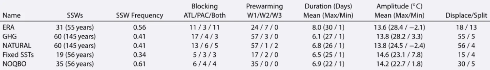
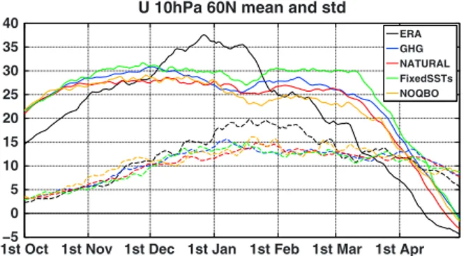
In this study we investigate how different natural and anthropogenic factors, namely, the quasi-biennial oscillation (QBO), sea surface temperatures (SSTs), anthropogenic greenhouse gases, and ozone-depleting substances, influence the frequency, variability, and life cycle of major warmings. This is done using sensitivity experiments performed with the National Center for Atmospheric Research’s Community Earth System Model (CESM). CESM is able to simulate the life cycle of major warmings realistically. The QBO strengthens the climatological stratospheric polar night jet (PNJ) and significantly reduces the frequency of major warmings through reduction of planetary wave propagation into the PNJ region. Variability in SSTs weakens the PNJ and significantly increases the major warming frequency due to enhanced wave forcing.
Even extreme climate change conditions (RCP8.5 scenario) do not influence the total frequency but determine the prewarming phase of major warmings. The amplitude and duration of major warmings seem to be mainly determined by internal stratospheric variability. We also suggest that SST variability, two-way ocean/atmosphere coupling, and hence the memory of the ocean are needed to reproduce the observed tropospheric negative Northern Annular Mode pattern after major warmings.
1. Introduction
Stratospheric sudden warmings (SSWs) are prominent disturbances of the Northern Hemisphere (NH) winter stratospheric polar vortex and are also a clear manifestation of the dynamical coupling in the stratosphere-troposphere system. They were first discovered byScherhag[1952] and are induced by the interaction of upward propagating planetary waves of tropospheric origin with the zonal mean flow [Matsuno, 1971]. By this interaction, the vortex is disrupted in its zonal symmetry and displaced from the pole or split into two vortices, leading to increased temperatures in the polar stratosphere. If additionally the wind at 60◦N, 10 hPa reverses from westerly to easterly, the warming is called a major warming, according to the definition of the World Meteorological Organization (WMO;Labitzke and Naujokat[2000]). The signa- ture of major sudden warmings can descend to the troposphere and thus even affect surface weather and climate [Quiroz, 1977;Baldwin and Dunkerton, 2001;Thompson et al., 2002;Mitchell et al., 2013]; therefore, the accurate simulation of SSWs and their downward propagating dynamical disturbances yield potential for improving the tropospheric weather prediction skill in climate models [Baldwin and Dunkerton, 2001;
Thompson et al., 2002;Mitchell et al., 2013].
A major warming is observed about every 2 years [Erlebach et al., 1996;Labitzke and Naujokat, 2000;
Charlton and Polvani, 2007], thoughLabitzke[1977],Labitzke and Naujokat[2000], andSchimanke et al.
[2011] pointed out (in observations and a model study, respectively) that SSW occurrence has large interannual to interdecadal variability. SSWs dominate the interannual variability of the NH polar winter stratosphere [Labitzke and Naujokat, 2000]. There are various natural and anthropogenic factors that influ- ence both the mean state and the variability of the polar vortex, suggesting a possible impact of these forcings on SSWs. Natural factors include, e.g., the quasi-biennial oscillation (QBO) of equatorial stratospheric winds, variations in sea surface temperatures (SSTs) such as the El Ni ˜no Southern Oscillation (ENSO), the 11 year solar cycle, and volcanic eruptions. Anthropogenic factors involve changes in greenhouse gases
(GHGs) and ozone-depleting substances (ODSs). By affecting either the background winds, the generation and propagation of waves, or the wave-mean flow interaction, these factors impact the polar vortex and hence the frequency and characteristics of SSWs. These dynamical mechanisms are not yet well understood and will be investigated in this study for some of the above mentioned factors.
The influence of the QBO on the polar stratosphere was first examined byHolton and Tan[1980, 1982]. On average, the polar stratospheric vortex is colder and less disturbed in QBO west-phase winters, leading to a lower frequency of SSWs, while winters during QBO east phase tend to be warmer and more disturbed, and more SSWs are observed. The mechanism behind this is not fully understood yet; it is likely that both the position of the zero wind line (known as the Holton-Tan mechanism;Holton and Tan[1980, 1982];Watson and Gray[2014]) and also the QBO-induced secondary meridional circulation [Naoe and Shibata, 2010;
Garfinkel et al., 2012] influence the propagation of planetary waves which are then responsible for the stronger or weaker disturbance of the polar vortex.
The influence of SST variations on the polar vortex largely happens within ENSO events.Van Loon and Labitzke[1987] found in observations that warm ENSO events (El Ni ˜nos) seem to be associated with an anomalously weak and warm polar vortex and hence more SSWs.Manzini et al.[2006] confirmed in a model study the statistical significance of this relationship and also highlighted its nonlinear character, i.e., that cold ENSO events (La Ni ˜nas), on the other hand, do not have an equivalent influence significantly dis- tinguishable from internal variability. This was also confirmed in model studies by, e.g.,Sassi et al.[2004]
andTaguchi and Hartmann[2006] and observational studies byCamp and Tung[2007] andMitchell et al.
[2011]. By analyzing general circulation model simulations,Manzini et al.[2006] andAyarzagüena et al.
[2013] suggested that the large-scale, extratropical ENSO teleconnection pattern in NH winter includes a deepening of the Aleutian low during El Ni ˜no events which enhances the forcing and vertical propagation of quasi-stationary planetary waves, resulting in a weaker stratospheric polar vortex. However,Butler and Polvani[2011] andGarfinkel et al.[2012] found that the SSW frequency is enhanced during both El Ni ˜no and La Ni ˜na years in reanalysis data and climate model simulations, despite the opposite-signed influence of the ENSO phases on the polar vortex. In general, two-way coupling between the atmosphere and the ocean in climate models has been shown to increase the low-frequency variability in both media [Barsugli and Battisti, 1998]. Recently,Omrani et al.[2014] suggested in a model study that decadal variability in North Atlantic SSTs might influence stratospheric background winds and SSWs.
Other natural factors that modify the polar vortex and hence may affect the frequency of SSWs directly or by interaction with other factors are the 11 year solar cycle [e.g.,Gray et al., 2010] and volcanic eruptions [e.g., Robock, 2000].
The influence of anthropogenic GHGs and ODSs on the polar vortex and SSWs is mainly addressed in model studies using 21st century GHG emission scenarios and comparing them to observations or model simulations of the 20th century. The results are, however, not concordant: while the majority of recent studies shows an increase in SSW frequency under increased GHG forcings [e.g.,Huebener et al., 2007;
Charlton-Perez et al., 2008;Bell et al., 2009;Schimanke et al., 2013;Ayarzagüena et al., 2013], one general circu- lation model study shows a decrease [Rind et al., 1998] and others no significant trend [Butchart et al., 2000;
SPARC CCMVal, 2010;Mitchell et al., 2012]. Possible causes for changes in SSW frequency under increased GHG conditions are found to be changes in the stratospheric meridional overturning circulation, which itself occurs due to a combination of changes in wave flux from the troposphere into the stratosphere [Ayarzagüena et al., 2013;Schimanke et al., 2013], and changes in middle atmospheric zonal winds [McLandress and Shepherd, 2009;Schimanke et al., 2013].
There are still a number of open questions about the influence of natural and anthropogenic factors on the polar vortex and the frequency of SSWs. Nonlinear interactions between the single forcing factors compli- cate the gain of insight, e.g., because QBO east years tend to coincide with El Ni ˜no years. Since observational records of the stratosphere are short and it is complicated if not impossible to separate the influence of the respective factors, we designed sensitivity simulations with a high-top stratosphere-resolving chemistry- climate model (CCM) to systematically switch on and off the single factors and analyze their respective roles.
We use National Center for Atmospheric Research (NCAR)’s Community Earth System Model (CESM) ver- sion 1.0.2, a state-of-the-art coupled model system with the Whole Atmosphere Community Climate Model (WACCM) version 4 as its atmospheric component.