The importance of interactive chemistry for stratosphere–troposphere coupling

(1)

https://doi.org/10.5194/acp-19-3417-2019

The importance of interactive chemistry for stratosphere–troposphere coupling

Sabine Haase¹and Katja Matthes^1,2

1GEOMAR Helmholtz Center for Ocean Research Kiel, Kiel, Germany

2Faculty of Mathematics and Natural Sciences, Christian-Albrechts-Universität zu Kiel, Kiel, Germany Correspondence:Sabine Haase (shaase@geomar.de)

Received: 1 October 2018 – Discussion started: 25 October 2018

Revised: 25 January 2019 – Accepted: 15 February 2019 – Published: 18 March 2019

Abstract. Recent observational and modeling studies suggest that stratospheric ozone depletion not only influences the surface climate in the Southern Hemisphere (SH), but also impacts Northern Hemisphere (NH) spring, which im- plies a strong interaction between dynamics and chemistry. Here, we systematically analyze the importance of interactive chemistry with respect to the representation of stratosphere–troposphere coupling and in particular the effects on NH surface climate during the recent past. We use the interactive and specified chemistry version of NCAR’s Whole Atmosphere Community Climate Model coupled to an ocean model to investigate differences in the mean state of the NH stratosphere as well as in stratospheric extreme events, namely sudden stratospheric warmings (SSWs), and their surface impacts. To be able to focus on differences that arise from two-way interactions between chemistry and dynamics in the model, the specified chemistry model version uses a time-evolving, model-consistent ozone field generated by the interactive chemistry model version. We also test the effects of zonally symmetric versus asymmetric prescribed ozone, evaluating the importance of ozone waves in the representation of stratospheric mean state and variability.

The interactive chemistry simulation is characterized by a significantly stronger and colder polar night jet (PNJ) during spring when ozone depletion becomes important. We identify a negative feedback between lower stratospheric ozone and atmospheric dynamics during the breakdown of the stratospheric polar vortex in the NH, which contributes to the different characteristics of the PNJ between the simulations.

Not only the mean state, but also stratospheric variability is better represented in the interactive chemistry simulation, which shows a more realistic distribution of SSWs as well as

a more persistent surface impact afterwards compared with the simulation where the feedback between chemistry and dynamics is switched off. We hypothesize that this is also related to the feedback between ozone and dynamics via the intrusion of ozone-rich air into polar latitudes during SSWs.

The results from the zonally asymmetric ozone simulation are closer to the interactive chemistry simulations, imply- ing that under a model-consistent ozone forcing, a three- dimensional (3-D) representation of the prescribed ozone field is desirable. This suggests that a 3-D ozone forcing, as recommended for the upcoming CMIP6 simulations, has the potential to improve the representation of stratospheric dynamics and chemistry. Our findings underline the importance of the representation of interactive chemistry and its feedback on the stratospheric mean state and variability not only in the SH but also in the NH during the recent past.

1 Introduction

Ozone is a key constituent of the stratosphere and is important not only for stratospheric chemistry, but also for transport and dynamics. Ozone is mainly produced in the trop- ics and transported towards higher latitudes by the large- scale meridional circulation in the middle atmosphere, i.e., the Brewer–Dobson circulation (BDC). This transport, which is directed towards the winter hemisphere, leads to a larger concentration of ozone at high latitudes compared with lower latitudes. The production of ozone and the absorption of UV radiation by stratospheric ozone leads to the characteristic increase of the stratospheric temperature with height, resulting in a stable stratification. Hence, ozone and its photochem-

(2)

ical characteristics are important for the seasonal cycle of stratospheric temperatures and due to their influence on the meridional temperature gradient also affect stratospheric circulation and dynamics through the thermal wind balance.

Consequently, a large interannual variability or anomalous trends in stratospheric ozone have the potential to influence the stratospheric mean dynamical state, its variability, and stratosphere–troposphere coupling (STC), which can impact the surface climate. The importance of the interactive representation of stratospheric ozone in a state-of-the-art climate model for STC is addressed here.

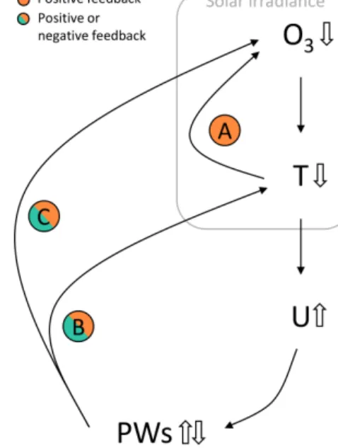
It is well known that polar ozone depletion during spring leads to a cooling of the lower stratosphere via radiative heating anomalies (Fig. 1). This cooling then enhances cat- alytic ozone depletion, as heterogeneous chemistry is more efficient at lower temperatures (A in Fig. 1). Thus, it de- scribes a positive feedback based on the interaction between ozone chemistry and the absorption of solar radiation (Ran- del and Wu, 1999). However, there is also a dynamical response to ozone depletion: lower polar temperatures enhance the meridional temperature gradient and, therefore, increase the strength of the polar night jet (PNJ) through thermal wind balance which in turn influences planetary wave propagation and dissipation. Depending on the strength of the PNJ, upward planetary wave propagation and dissipation can either be enhanced or diminished (Charney and Drazin, 1961). This has opposing effects on the state of the polar vortex and can lead to either positive or negative feedbacks between ozone depletion and stratospheric dynamics (B and C in Fig. 1) (e.g., Mahlman et al., 1994; Manzini et al., 2003; Lin et al., 2017). Therefore, the strength of the background wind de- termines the impact of ozone depletion on planetary wave propagation and dissipation and, in turn, the sign of the feedback.

If we consider an initial cooling due to ozone depletion and strong westerly background winds, the cooling would result in a further strengthening of the background winds; this, in turn, would hinder upward planetary wave propagation and result in a positive feedback. If the cooling from ozone depletion was accompanied by weak westerly background winds, it would also result in a strengthening of the background winds; however, in that case it would favor planetary waves propagating upward and would consequently result in a negative feedback. Stronger (weaker) upward planetary wave propagation results not only in a weakening (strengthening) of the PNJ but also in a strengthening (weakening) of the downwelling branch of the BDC, which can both directly or indirectly influence stratospheric ozone concentrations. A stronger (weaker) descent over the pole leads to adiabatic warming (cooling) that counteracts (enhances) the negative temperature anomalies induced by ozone depletion (B in Fig. 1). Stronger (weaker) descent also increases (de- creases) the transport of ozone from higher altitudes to lower altitudes, increasing (decreasing) lower stratospheric ozone concentrations (C in Fig. 1). The same effect is achieved by

Figure 1. Scheme of possible feedbacks between ozone chemistry and dynamics/transport. A negative anomaly in ozone (O₃) will lead to a negative anomaly in temperature (T) which fa- vors ozone depletion (A – positive feedback). It also increases the strength of the polar night jet (U). Depending on the strength of the background westerlies, an increase inU can lead to either an increase or decrease in upward planetary wave propagation (PWs).

A strong (weak) westerly background wind can lead to a decrease (increase) in PWs, which is connected to a less (more) disturbed polar vortex, coupled to (B) a cooling (warming) of the polar vortex, and (C) to less (more) transport of ozone into the polar vortex.

Consequently, strong (weak) background westerlies are connected to positive (negative) feedbacks between ozone chemistry and dynamics/transport (B and C).

the weaker (stronger) PNJ, which allows for more (less) mixing between ozone depleted polar air masses and the relatively ozone-rich surrounding air masses. These feedbacks would therefore be negative (positive) (B and C in Fig. 1).

The impact of ozone depletion on stratospheric dynamics is strongest during spring (when solar irradiance is available to initiate ozone depletion) and, following our discussion above, is very sensitive to the background state of the polar vortex. In fact, previous studies have suggested a dom- inance of the negative feedback during the vortex breakdown (e.g., Manzini et al., 2003; Lin et al., 2017).

Although other trace gases, such as water vapor, can also be affected by these feedbacks, we concentrate our discussion on ozone in this publication. The effects of ozone can be represented differently in climate models: the most so- phisticated representation is to calculate ozone interactively within the model’s chemistry scheme. Ozone, as well as many other trace gases and chemicals, is thereby directly and interactively linked to the radiation and dynamics. These climate models are called chemistry–climate models (CCMs) and are used for stratospheric applications such as in the

(3)

WCRP/SPARC initiatives. However, fully interactive atmospheric chemistry schemes are computationally expensive, particularly if an interactive ocean is also used for long- term climate model simulations. Therefore, an alternative way of representing the effects of ozone chemistry in a climate model is to prescribe ozone fields which can be based on either observed or modeled ozone concentrations. These ozone fields can be of different temporal and horizontal resolution. The majority of climate models that participated in the Climate Model Intercomparison Project, Phase 5, (CMIP5), prescribe ozone as monthly mean, zonal mean values (Eyring et al., 2013) based on the recommended IGAC/SPARC ozone database (Cionni et al., 2011).

When prescribing ozone as monthly mean, zonal mean fields, some aspects of ozone variability, such as zonal asymmetries in ozone, are neglected. Using a monthly climatology has been shown to introduce biases in the model’s ozone field that reduce the strength of the actual seasonal ozone cycle due to the interpolation of the prescribed ozone field to the model time step (Neely et al., 2014). To avoid these biases, a daily ozone forcing can be applied. Furthermore, ozone is not distributed in a zonally symmetric fashion in the real atmosphere; therefore, prescribing zonal mean ozone values inhibits the effect that zonal asymmetries in ozone, also referred to as ozone waves, can have on the dynamics. Different studies have shown that including zonal asymmetries in ozone in a model simulation leads to a warmer and weaker stratospheric polar vortex in the NH, which has also been associated with a higher frequency of SSWs (e.g., Gabriel et al., 2007; Gillett et al., 2009; McCormack et al., 2011; Peters et al., 2015). The recommended ozone forcing for CMIP6 now includes zonal asymmetries, but does not include variability on timescales shorter than a month (Checa- Garcia et al., 2018).

As the interactive chemistry module in a climate model is computationally very expensive, it is necessary to elucidate alternative representations of ozone for long-term climate simulations. To date, the importance of interactive chemistry in climate models has mainly been evaluated for experimental settings that have focused on the effect of an altered external forcing, such as a change in solar irradiance or CO₂ concentrations (e.g., Chiodo and Polvani, 2016, 2017; Diet- müller et al., 2014; Noda et al., 2018; Nowack et al., 2017, 2018b). In these studies CCM simulations were compared to model simulations forced with a constant ozone field (e.g., based on preindustrial control conditions), which did not include the ozone response to the changing external forcing. It was shown that the ozone response to the external forcing has an important damping effect on the surface climate response to the external forcing. That is to say, under such conditions, including interactive chemistry reduces the model’s climate sensitivity (e.g., Chiodo and Polvani, 2016; Dietmüller et al., 2014; Noda et al., 2018; Nowack et al., 2018b) and connected surface responses, such as the tropospheric jet (e.g.

Chiodo and Polvani, 2017) or El Niño–Southern Oscillation

trends (e.g., Nowack et al., 2017). Here, we use a different approach. We are interested in how feedbacks between ozone chemistry and model dynamics can impact the stratospheric mean state and variability, given that the variability in stratospheric ozone is the same between the interactive and specified chemistry experiments. This question will be addressed in the present study using a time-evolving, model- consistent ozone forcing in the specified chemistry version of the model.

When considering the impact of ozone on stratospheric dynamics one has to distinguish between the two hemispheres.

During Antarctic winter, temperatures are very low and reach the threshold for polar stratospheric cloud (PSC) formation every winter. This allows the heterogeneous chemical loss of polar ozone via ozone depleting substances (ODSs) once sunlight returns in spring and leads to the well-known formation of the Antarctic ozone hole every austral spring.

Although the Montreal Protocol regulated the emissions of ODSs, they have a very long lifetime and continue to de- plete ozone every winter, which is most prominently seen in the last 2 decades of the 20th century. The ozone hole contributes to a positive trend in the southern annular mode during austral summer (December to February, DJF), which influences the position and strength of the tropospheric jet and consequently impacts the surface wind stress forcing on the Southern Ocean (e.g., Son et al., 2008; Thompson et al., 2011; Previdi and Polvani, 2014).

Recently, Son et al. (2018) evaluated the representation of the observed SH ozone trend and the resulting poleward shift of the tropospheric jet in the latest CCMs and high-top CMIP5 models (model top at or above 1 hPa). They argued that irrespective of the representation of stratospheric ozone (prescribed or interactive) the poleward shift of the tropospheric jet due to ozone depletion was captured in all model ensembles. Separating the CMIP5 models with and without interactive chemistry showed a slightly stronger poleward trend in zonal mean zonal wind during DJF in the models with interactive chemistry. However, Son et al. (2018) also point out that the inter-model spread in the tropospheric jet latitude trend is rather high; it is positively correlated with the strength of the ozone trend in individual CCMs but also dependent on different model dynamics. Hence, it is more convenient to use one model with the same dynamics to investigate the effect of interactive chemistry. For example, Li et al. (2016) focused on one model, the Goddard Earth Ob- serving System Model version 5 (GEOS-5), to assure that the same dynamical background was used between simulations; their study found a significantly stronger trend in zonal mean zonal wind in austral summer and a more significant surface response in surface wind stress and ocean circulation to the same ozone trends when ozone was calculated interactively in the model. There are only a few studies, such as Li et al. (2016), which are designed to systematically compare the effect of including or excluding interactive chemistry in the same model, i.e., also using the ozone forcing from the

(4)

CCM in the specified chemistry version of the model. How- ever, there is still a great need to better understand the role that feedbacks between chemistry and dynamics may play in representing recent and also future climate conditions on different timescales.

Recently, Lin et al. (2017) discussed the negative feedback between ozone depletion and dynamics (recall Fig. 1) in detail for the observed SH ozone trend, showing that the lower stratospheric dynamical response to ozone depletion depends on the timing of the climatological vortex breakdown during spring. They also claimed that models with a cold-pole bias overestimate the effect of SH ozone depletion due to an un- derestimation of the negative feedback. Here, we want to investigate how important the representation of such feedbacks in a climate model is for Northern Hemisphere (NH) stratospheric dynamics and whether it can impact the tropospheric circulation via extreme stratospheric events.

In the NH, where the stratospheric polar vortex is much more disturbed and, therefore, warmer during winter, a clear trend in either total column or lower stratospheric ozone is not as prominent as in the SH. Very low ozone concentrations dominated in the 1990s (Ivy et al., 2017), but more recent years, such as 2011, have also exhibited extremely low Arc- tic spring ozone concentrations (Manney et al., 2011). This event (in 2011) in particular initiated discussions about the possibility of an Arctic ozone hole and also about the possible impact of NH ozone depletion events on the surface (Che- ung et al., 2014; Karpechko et al., 2014; Smith and Polvani, 2014). Using different models but all with prescribed ozone, these studies did not find a significant surface impact from observed ozone anomalies. In particular, Smith and Polvani (2014) reported that significantly higher NH ozone depletion than that observed in 2011 would be needed to cause a detectable surface impact. Conversely, Calvo et al. (2015) reported statistically significant impacts of NH ozone depletion events on tropospheric winds, surface temperatures, and precipitation in April and May using the same CCM (WACCM) as used in this study. This suggests that feedbacks between dynamics and chemistry are necessary to induce a tropospheric signal due to ozone depletion in the NH. In this study, we will test the importance of two-way feedbacks between ozone chemistry and dynamics for NH STC in recent decades.

Extreme events in the NH stratosphere can have strong and relatively long-lasting impacts on the troposphere (e.g.

Baldwin and Dunkerton, 2001) and are therefore of great interest, for example, for seasonal weather prediction (e.g.

Baldwin et al., 2003; Sigmond et al., 2013). Different pathways have been proposed to explain the coupling between the stratosphere and the troposphere, including the wave–mean- flow interaction, wave refraction and reflection mechanisms (e.g., Haynes et al., 1991; Hartmann et al., 2000; Perlwitz and Harnik, 2003; Song and Robinson, 2004), as well as potential vorticity change (Ambaum and Hoskins, 2002; Black, 2002).

Understanding the relative contribution of these mechanisms

to STC in detail is still the subject of recent research. Here, we focus on sudden stratospheric warmings (SSWs) as a prominent example of NH STC. SSWs are characterized by a strong wave-driven disturbance or breakdown of the stratospheric polar vortex and result in a surface response a few days after the onset of the stratospheric event that resembles the pattern of the negative phase of the North Atlantic Oscil- lation (NAO) (Baldwin and Dunkerton, 2001). A systematic investigation of interactive vs. prescribed ozone in the same climate model family on NH STC effects has to our knowl- edge not yet been performed and is the goal of the present study.

Apart from the representation of two-way feedbacks between chemistry and dynamics, also zonal asymmetry in ozone is often not included when ozone and other radiatively active species are prescribed. However, earlier publications have shown that zonally asymmetric ozone is associated with a warmer and weaker stratospheric polar vortex in the NH (e.g. Gillett et al., 2009; McCormack et al., 2011; Albers and Nathan, 2012; Peters et al., 2015) compared with zonal mean ozone conditions. Gillett et al. (2009), for example, showed that the NH polar stratospheric vortex is warmer when using zonally asymmetric ozone compared with zonal mean ozone in the radiation scheme. In their model setup feedbacks between dynamics and zonal mean ozone concentrations were possible, only the effects of ozone waves were inhibited. A significant warming of the polar stratosphere was only found in early winter (November and December). Using a similar model setup, McCormack et al. (2011) found a more significant warming in February when including zonally asymmetric ozone in their model and associated it with the more prevalent occurrence of SSWs in their experiments The total number of SSWs was rather low with only five out of thirty ensemble members: four out of the five SSWs occurred in the zonally asymmetric simulations. Peters et al. (2015) prescribed ozone in both simulations and also found a higher occurrence of SSWs in the zonally asymmetric ozone run, with the largest difference in SSW occurrence in November.

Furthermore, a recent study by Silverman et al. (2018) points to the importance of the Quasi-Biennial Oscillation (QBO) for the NH high-latitude response to ozone waves. To test the sensitivity of using either a zonal mean ozone field or a zonally asymmetric field, we additionally include a sensitivity experiment using a 3-D ozone forcing in the specified chemistry simulation.

The paper is organized as follows: Sect. 2 introduces the model and the simulations performed in this study in addition to the methodologies applied. After discussing the differences in the climatological mean state between interactive and prescribed chemistry model simulations in Sect. 3, we analyze the differences in SSW characteristics and downward influences between the simulations in Sect. 4. Finally, we conclude the paper with a discussion of our results.

(5)

2 Data and methods 2.1 Model simulations

To asses the importance of interactive chemistry on the mean state and variability of the stratosphere as well as on STC, we use a model that is capable of utilizing an interactive chemistry scheme as well as specified chemistry.

We use the Community Earth System Model (CESM), version 1, from NCAR with WACCM, version 4, as the atmospheric component; this setting is referred to as CESM1(WACCM). This version of CESM1(WACCM) is documented in detail in Marsh et al. (2013).

WACCM is a fully interactive chemistry–climate model, with a horizontal resolution of 1.9^◦latitude×2.5^◦longitude.

It uses a finite volume dynamical core, has 66 vertical levels with variable spacing, and an upper lid at 5.1×10⁻⁶hPa (about 140 km) that reaches into the lower thermosphere (Garcia et al., 2007). Stratospheric variability, such as SSW properties and the evolution of the SH ozone hole are well captured in CESM1(WACCM) (Marsh et al., 2013). In the SH, CESM1(WACCM) has a strong cold-pole bias in the middle atmosphere, which could influence the feedbacks discussed in Fig. 1 (Lin et al., 2017). In the NH, the strength of the PNJ agrees well with observations (Richter et al., 2010);

therefore, the NH is better suited to investigate these feedbacks.

For our investigations we run the model under historical forcing conditions for the period from 1955 to 2005 and under the Representative Concentration Pathway 8.5 (RCP8.5) from 2006 to 2019. Therefore, we capture a 65-year period that features the years with the lowest ozone concentrations before ozone recovery starts. We include all external forcings based on the CMIP5 recommendations: greenhouse gas (GHG) and ODS concentrations (Meinshausen et al., 2011), spectral solar irradiances (Lean et al., 2005), and volcanic aerosol concentrations (Tilmes et al., 2009) including the eruptions of Agung (1963), El Chichón (1982), and Mount Pinatubo (1991). As the QBO is not generated internally by this version of WACCM, it was nudged following the methodology of Matthes et al. (2010).

CESM1(WACCM) incorporates an active ocean (Parallel Ocean Program version 2, POP2), land (Community Land Model version 4, CLM4), and sea ice (Community Ice CodE version 4, CICE4) model. POP2 and CICE4 have a nominal latitude–longitude resolution of 1^◦; the ocean model has 60 vertical levels. A central coupler is used to exchange fluxes between the different components. For more details on the different model components the reader is referred to Hurrell et al. (2013) and references therein.

As mentioned above, WACCM incorporates an interactive chemistry scheme in its standard version. It uses version 3 of the Model for Ozone and Related Chemical Tracers (MOZART) (Kinnison et al., 2007). Within MOZART ozone concentrations and concentrations of other radiatively active

species are calculated interactively, which allows for feedbacks between dynamics and chemistry as well as radiation.

It includes the O_x, NO_x, HO_x, ClO_x, and BrO_x chemical families, along with CH_xand its degradation products. A total of 59 species and 217 gas-phase chemical reactions are represented, and 17 heterogeneous reactions on three aerosol types are included (Kinnison et al., 2007).

The specified chemistry version of WACCM (SC- WACCM), in which interactive chemistry is turned off, does not simulate feedbacks between chemistry and dynamics.

This version of WACCM is documented in Smith et al.

(2014). Here, ozone concentrations are prescribed throughout the whole atmosphere. Above approximately 65 km, in addition to the ozone concentrations, concentrations of other species, namely atomic and molecular oxygen, carbon diox- ide, nitrogen oxide, and hydrogen, as well as the total shortwave and chemical heating rates are also prescribed. Smith et al. (2014) validated SC-WACCM by prescribing monthly mean zonal mean values of the aforementioned species and heating rates from a companion WACCM run. Following the procedure in Smith et al. (2014), we use the output from our transient WACCM integration to specify all of the necessary components in SC-WACCM (i.e., O, O₂, O₃, NO, H, CO₂, and total shortwave and chemical heating rates). We use transient, monthly mean zonal mean values for all variables, ex- cept ozone, for which we use daily zonal mean transient data.

The use of daily ozone data reduces a bias that is introduced by linear interpolation of the prescribed ozone data to the model time step when using monthly ozone values (Neely et al., 2014). Using daily data also allows for extreme ozone anomalies to occur in the specified chemistry run.

In the following we will refer to the interactive chemistry version of CESM1(WACCM) as “Chem ON” and to the specified version, that uses SC-WACCM as the atmosphere component, as “Chem OFF”. Additionally, we include results from a sensitivity run, prescribing daily zonally asymmetric (3-D) transient ozone in SC-WACCM, which will be referred to as Chem OFF 3D. All other settings in Chem OFF 3D are equal to that of the Chem OFF simulation. The model simulations and settings are summarized in Table 1.

2.2 Methods

The results presented in this paper are largely based on climatological mean values of model output. When variability is considered we use deseasonalized daily or monthly data by removing a slowly varying climatology after removing the global mean from each grid point each year. This follows the procedure described in Gerber et al. (2010) and is used to omit the effect that may arise from variability on timescales longer than 30 years, such as the signature of global warming. The slowly varying climatology is produced as follows:

first, a 60-day low-pass filter is applied. Then, for each time step and grid point, a 30-year low-pass filter is applied to the smoothed time series. Gerber et al. (2010) describe this

(6)

Table 1.Model experiments carried out with CESM1(WACCM) in Chem ON, Chem OFF, and Chem OFF 3D mode. For more details see text.

Experiment/ Ozone setting Years SSWs during winters of

data 1955/56 to 2018/19 1958/59 to 2016/17

Chem ON Interactive 1955 to 2019 26 24

Chem OFF Prescribed^∗zonal mean 1955 to 2019 41 40

Chem OFF 3D Prescribed^∗zonally asymmetric 1955 to 2019 30 28

ERA – 1958 to 2017 – 32

∗The ozone data used for prescription originate from the Chem ON run.

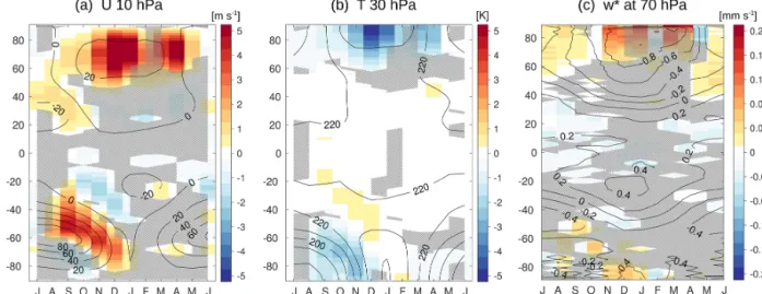
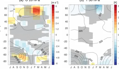
Figure 2.Climatological zonal mean(a)zonal wind at 10 hPa in m s⁻¹,(b)temperature at 30 hPa in K, and(c)w^∗at 70 hPa in mm s⁻¹ with month and latitude for Chem OFF (contours) and for the difference between Chem ON and Chem OFF (shading). Contour intervals are (a)20 m s⁻¹,(b)10 K, and(c)0.2 mm s⁻¹. Statistically insignificant areas are hatched at the 95 % level.

Figure 3.February–April (FMA) zonal mean(a)zonal wind in m s⁻¹and(b)temperature in K with latitude and height for the NH for Chem OFF (contours) and for the difference between Chem ON and Chem OFF (shading). Contour intervals are(a)10 m s⁻¹and(b)10 K. Solid contours are used for positive values, and dashed contours are used for negative values. The zero line is omitted. Statistically insignificant areas are hatched at the 95 % level.

procedure in detail and apply it exemplarily. We confine the results presented to altitudes below 5 hPa, as it is the lower stratospheric ozone and its effects on the circulation that we are most interested in.

We calculated the vertical component of the meridional residual circulation (w^∗) using the transformed Eulerian mean framework defined, for example, in Andrews et al.

(1987):

(7)

w^∗=w+ 1 Acosφ

cosφv⁰2⁰ 2⁰_z

φ

, (1)

where the overbar indicates zonal mean values, subscripts refer to partial derivatives, A denotes the Earth’s radius (A=6 371 000 m), andw^∗is used to estimate the difference in tropical upwelling and polar downwelling between the model simulations. We refer to major sudden stratospheric warmings as “SSWs” or “major warmings” in the following. SSWs are defined based on the definition from the World Meteorological Organization (WMO) (e.g., McInturff, 1978;

Andrews et al., 1987); according to this definition, they occur (between November and March) when the two following criteria are fulfilled: (1) the predominantly westerly zonal mean zonal wind reverses sign at 60^◦N and 10 hPa, i.e., changes from westerly to easterly; and (2) the 10 hPa zonal mean temperature difference between 60^◦N and the pole is positive for at least 5 consecutive days. The central date (or onset) of SSWs is defined as the first day of wind reversal. To exclude final warmings (the transition from winter to summer circulation), a switch from westerly to easterly winds at the given location is only considered a SSW if the westerly wind recov- ers for at least 10 consecutive days prior to 30 April (Charlton and Polvani, 2007) and exceeds a threshold of 5 m s⁻¹(Ban- calá et al., 2012). To avoid double counting of events, there have to be at least 20 days of westerlies in between two major warmings (Charlton and Polvani, 2007).

We compare the modeled major warming frequency to the European Centre for Medium-Range Weather Forecasts Re- Analysis (ERA) products ERA40 (Uppala et al., 2005) and ERA-Interim (Dee et al., 2011). These two products were combined into one data set following Blume et al. (2012) (here merged on 1 April 1979), which resolves the stratosphere up to 1 hPa and spans the period from 1958 to 2017.

Regarding the uncertainty estimate for the SSW frequencies, we use the standard error for the monthly frequencies and the 95 % confidence interval based on the standard error for the winter mean frequency.

Atmospheric variability linked to SSWs is evaluated in the form of composites for selected variables before, during, and after the SSW onset. The statistical significance of the composites is tested using a Monte Carlo approach (see for example von Storch and Zwiers, 1999). Therefore, 10 000 randomly chosen central dates are used to calculate random composites. Statistical significance at the 95 % level is reached when the actual composites exceed the 2.5th or 97.5th percentiles of the distribution drawn from the random composites.

The differences between Chem ON and Chem OFF are displayed as Chem ON minus Chem OFF, and they are de- picted along with the climatological field of the Chem OFF run to display the effect of including interactive chemistry.

For these differences, the statistical significance at the 90 % or 95 % level is tested using a two-sidedttest.

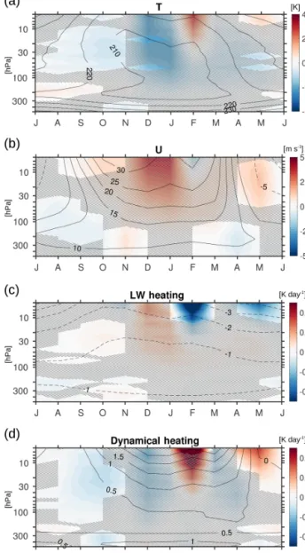
Figure 4.Climatological NH(a)polar cap (70 to 90^◦N) temperature in K,(b)zonal mean zonal wind (55 to 75^◦N) in m s⁻¹,(c)polar cap longwave heating rates in Kday⁻¹, and(d)polar cap dynamical heating rates in K day⁻¹with month and height for Chem OFF (contours) and for the differences between Chem ON and Chem OFF (shading). Contour intervals are(a)10 K,(b)5 m s⁻¹, (c)1 K day⁻¹, and(d)0.5 K day⁻¹. Solid contours are used for positive values, and dashed contours are used for negative values. The zero contour is omitted. Statistically insignificant areas are hatched at the 95 % level.

3 The impact of interactive chemistry on the stratospheric mean state

To assess the importance of interactive chemistry on stratospheric dynamics we first consider zonal mean zonal wind at 10 hPa (U10) and zonal mean temperature at 30 hPa (T30) to characterize the stratospheric polar vortex in our model simulations (Fig. 2a, b). The stratospheric PNJ is character-

(8)

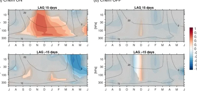
Figure 5.Correlation between polar cap (70 to 90^◦N) ozone at 50 hPa and polar cap dynamical heating rates in(a)Chem ON and(b)Chem OFF for ozone lagging by 15 days (LAG 15 days) and ozone leading by 15 days (LAG−15 days). Statistically insignificant areas are hatched at the 95 % level.

ized by strong westerlies around 70^◦N and 60^◦S (Fig. 2a) and low polar cap temperatures (Fig. 2b). The PNJ is significantly stronger and colder in the Chem ON run. In both hemispheres, this feature is especially significant during spring, when ozone chemistry becomes important for the temperature budget of the lower stratosphere and hence for the dynamics. This difference already hints at the relevance of representing feedbacks between ozone chemistry and dynamics for the climatological state of the PNJ during spring. In the NH, the difference between the runs is also significant during fall and early winter, which is connected to a weaker downwelling, i.e., weaker adiabatic warming, indicated by the statistically significant positive anomaly inw^∗at 70 hPa (Fig. 2c) from June to December. At the same time, Chem ON is characterized by a slightly weaker tropical upwelling at 70 hPa, indicating that at least the shallow branch of the BDC (below 50 hPa) is weaker in Chem ON compared with Chem OFF.

In the following we will focus on the NH spring season as this is the period when the effect of ozone depletion and possible feedbacks between chemistry and dynamics become important. Figure 3 shows February to April (FMA) NH zonal mean zonal wind and zonal mean temperature with height. Consistent with Fig. 2, north of 70^◦N, we find a stronger PNJ (up to 4.5 m s⁻¹ stronger at about 10 hPa) when interactive chemistry is included (Fig. 3a) and a colder polar vortex, with a maximum difference between Chem ON and Chem OFF of −2.8 K at about 60 hPa directly at the pole (Fig. 3b). While temperature differences between Chem ON and Chem OFF are mainly restricted to the lower stratosphere, statistically significant differences in

zonal mean zonal wind reach up to about 4 hPa and even down to the surface.

As the temperature differences are decisive for the differences in zonal wind, we now consider the differences in polar cap heating rates between Chem ON and Chem OFF to investigate why the models differ in their climatological stratospheric state (Fig. 4). As already seen in Figs. 2 and 3, including interactive chemistry leads to a stronger PNJ and colder polar vortex, especially during spring but also during early winter (Fig. 4a, b). Figure 4a and c show that lower (higher) temperatures go along with weaker (stronger) longwave (LW) cooling in the Chem ON run. The difference in LW cooling between Chem ON and Chem OFF is directly connected to the temperature difference and works as a damping factor. By construction, there are no significant differences in the shortwave (SW) heating rates between Chem ON and Chem OFF that could explain the different temperatures between the models in this region, nor can differences in temperature tendencies due to gravity waves (not shown). The dynamical heating rates, which describe the total adiabatic heating rates in the model dominated by ad- vection through the vertical component of the residual circulation, (w^∗), (Fig. 4d) seem to be the dominant factor in shaping the climatological differences in polar cap temperature between Chem ON and Chem OFF. Although the spring season is characterized by a stronger PNJ and lower polar cap temperatures in the lower stratosphere in Chem ON, a stronger dynamical heating in April and May leads to higher temperatures in Chem ON in the middle stratosphere peak- ing in May (Fig. 4a, d). Statistically significant dynamical heating differences between Chem ON and Chem OFF reach down to the troposphere resulting in a strong reduction of the

(9)

temperature difference between Chem ON and Chem OFF in the lower stratosphere in May. These features are characteristic of a later but more intense breakdown of the polar vortex when interactive chemistry is present. The differences in temperature between Chem ON and Chem OFF during early winter can also be explained by the differences in dynamical heating. In the Chem ON run there is statistically significant weaker dynamical warming compared with the Chem OFF run with a maximum difference between the runs in Novem- ber (Fig. 4d) that leads to lower temperatures in Chem ON in December. This agrees with the earlier finding that the shallow branch of the BDC is weaker in the Chem ON simulation (Fig. 2c). However, this poses the question as to why the signal in dynamical heating differs between early winter and late spring. We suggest feedbacks between ozone chemistry and dynamics as the reason for this and will discuss these factors in more detail in the following.

To illustrate the relation between ozone and dynamical heating we calculated the correlation between polar cap ozone concentrations at 50 hPa and polar cap dynamical heating rates in Chem ON and Chem OFF. A similar analysis using ozone and temperature was carried out by Lin et al.

(2017) for the SH. Figure 5 shows this correlation for ozone lagging and leading the dynamical heating rates by 15 days.

As the dynamical heating is only available at a monthly resolution, daily ozone data were shifted by±15 days with respect to the dynamical heating time axis. The contours show the climatological zonal mean zonal wind as a reference.

The shading shows the correlation coefficients. Two different states are represented in Fig. 5: (1) the dependence of ozone on the dynamics (Fig. 5, top row) and (2) the effect ozone can have on the dynamics (Fig. 5, bottom row). When ozone lags behind dynamical heating (Fig. 5a, top row), positive correlation coefficients occur in late autumn and early winter indicating that low (high) ozone concentrations follow low (high) dynamical heating rates. In this case, ozone concentrations and dynamical heating are caused by reduced (enhanced) downwelling which leads to adiabatic cooling (warming) as well as to lower (higher) ozone concentrations. When ozone leads dynamical heating (Fig. 5a, bottom row), positive correlation coefficients are not significant anymore. Instead, a statistically significant negative correlation between ozone and dynamical heating throughout the lower stratosphere is found in April and May, setting in earlier at higher altitudes (above 10 hPa). By only looking at the dynamical heating rates here, we do not capture possible positive feedbacks caused by radiative heating and ozone chemistry indicated under (A) in Fig. 1. Using this analysis we also do not identify a positive feedback between ozone chemistry and dynamics (recall B and C, Fig. 1). However, we clearly find a negative feedback between ozone and dynamics during the vortex breakdown phase in correspondence to earlier studies (e.g. Manzini et al., 2003; Lin et al., 2017). The westerly background wind is weak enough that a decrease in ozone concentrations leads to an increase in dynamical heating,

Figure 6.Same as Fig. 4 but using Chem OFF 3D for comparison with Chem ON.

which would consequently increase ozone concentrations via the aforementioned pathways (B and C, Fig. 1). This negative feedback indicates that during weak zonal mean zonal wind conditions, ozone depletion, which leads to an initial cooling of the lower polar stratosphere and strengthening of the PNJ, eventually leads to a faster breakdown of the vortex by allowing upward wave propagation to take place at a higher rate than would occur during weaker westerlies. In this analysis, the negative feedback clearly dominates and leads to a more abrupt breakdown of the polar vortex in the Chem ON simulation. A statistically significant correlation signature between ozone and dynamical heating is only found in Chem ON (compare Fig. 5a and b). Hence, we conclude that interactive chemistry is indeed contributing to the different

(10)

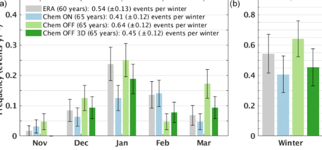
Figure 7.Monthly SSW frequency(a)and winter SSW frequency(b)for the combined ERA data (gray), Chem ON (blue), Chem OFF (light green), and Chem OFF 3D (dark green). Error bars are shown in the figure. They indicate the standard error for the monthly frequencies and the 95 % confidence interval based on the standard error for the mean winter frequency.

climatological characteristics of the PNJ between Chem ON and Chem OFF.

Apart from the lack of feedbacks between chemistry and dynamics, Chem OFF is also missing zonal asymmetry in the prescribed ozone field. Hence, the missing effect of ozone waves in the Chem OFF simulation could potentially contribute to the differences that we find between Chem ON and Chem OFF. Therefore, we also include a sensitivity run, for which we used a zonally asymmetric daily ozone forcing, Chem OFF 3D (Table 1).

When including ozone waves, no significant correlation signature is found between ozone and dynamical heating (similarly to Chem OFF; not shown). Nevertheless, the abso- lute climatological differences between Chem ON and Chem OFF 3D are smaller than what we found for a zonally symmetric ozone forcing (Figs. 4 and 6). The PNJ is still colder and stronger with interactive chemistry (Fig. 6a, b), and significant differences of the same sign as above are found for LW and dynamical heating rates in spring (Fig. 6c, d). The lower amplitude of the differences between Chem ON and Chem OFF 3D compared with Chem ON and Chem OFF do indicate that other processes (apart from the feedbacks discussed so far) are also important for the generally stronger and colder PNJ in Chem ON. Including zonal asymmetries in ozone generally allows for stronger anomalies in ozone, as no averaging is applied, and for anomalies that do not center over the pole but also affect lower latitudes. Hence, ozone waves can influence wave propagation and dissipation pathways, possibly leading to a better representation of the effect that ozone has on wave–mean-flow interactions in our model setup.

4 How does interactive chemistry influence stratosphere–troposphere coupling?

We found a stronger PNJ during NH spring when interactive chemistry and feedbacks between ozone and dynamics are included in a climate model. This stronger PNJ exhibits a boundary for upward planetary wave propagation which influences the occurrence of SSWs. Figure 7 shows the frequency of SSWs for ERA re-analysis data (gray), the Chem ON (blue), Chem OFF (light green), and Chem OFF 3D (dark green) simulations for each month of the extended winter season individually (Fig. 7a) and the average over the whole winter season (Fig. 7b) (see also Table 1). Chem ON rep- resents the observed monthly frequency of SSWs very well with the exception of January where it significantly underestimates the occurrence of SSWs. Chem OFF, in comparison, underestimates SSWs significantly in February and shows an unrealistic increase in the occurrence of SSWs towards the end of the extended winter season (March). Overall there is a tendency for fewer SSWs when interactive chemistry is included in the model (Chem ON: 0.41±0.12 warmings per winter; Chem OFF: 0.64±0.12 warmings per winter; and Ta- ble 1), which is likely due to the stronger background westerlies in Chem ON. The SSW frequency in Chem OFF 3D is much closer to that in Chem ON compared with Chem OFF, which we attribute to the smaller climatological differences between Chem ON and Chem OFF 3D. However, this poses the question as to how interactive chemistry impacts the downward influence of SSWs.

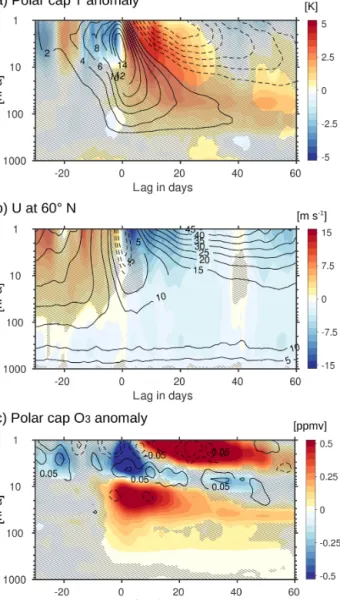
The downward propagation of anomalies connected to the vortex breakdown is stronger in the Chem ON simulation (Fig. 8). Polar cap temperature anomalies are stronger and persist longer in Chem ON (Fig. 8a). Furthermore, the zonal mean wind at 60^◦N (Fig. 8b) shows a longer-lasting easterly anomaly connected to SSWs that reaches further down to the surface. Figure 8a and b also demonstrate that the SSW

(11)

Figure 8. SSW composites for (a)the polar cap (60 to 90^◦N) temperature anomaly in K, (b) zonal mean zonal wind at 60^◦N in m s⁻¹, and for (c)the polar cap ozone anomaly in ppm with lag in days with respect to the SSW central date (lag 0) and height. Contour lines show the composite for the Chem OFF run.

Shading shows the difference between Chem ON and Chem OFF SSW composites. Contour intervals are(a)2 K,(b) 5 m s⁻¹, and (c) 0.05 ppmv. Solid contours are used for positive values, and dashed contours are used for negative values. The zero contour is omitted. Statistically insignificant areas are hatched at the 90 % level (two-samplettest).

signal in the Chem ON run is more sudden compared with the Chem OFF run: the polar cap temperature anomaly is significantly weaker before and significantly stronger after the SSW onset compared with the Chem OFF run. Also, the easterly wind at 60^◦N is preceded by stronger westerlies in the Chem ON simulation. Both criteria show a more abrupt change from before to after the central date. To consider the possible impact of ozone chemistry, we also show a compos-

ite of ozone volume mixing ratio anomalies during the SSWs (Fig. 8c). A strong intrusion of ozone from surrounding air masses during the SSWs, as described in de la Cámara et al.

(2018), is only evident in the Chem ON simulation. No significant signal is found in the Chem OFF run (contours in Fig. 8c). This suggests that the increase in lower stratospheric ozone in Chem ON contributes to the longer persistence of the SSW signal in the lower stratosphere.

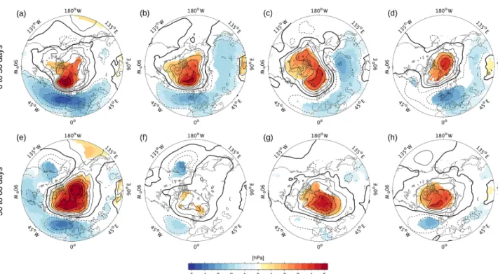
The stronger and more persistent SSW signal in the Chem ON run in the stratosphere also appears at the surface in the sea level pressure (SLP) response to SSWs (Fig. 9). The well- known negative NAO-like surface response after SSWs is stronger in the Chem ON simulation (averaged over 30 days after the SSW onset, Fig. 9a) and longer lasting (averaged over 30 to 60 days after the SSW onset, Fig. 9e) compared with the Chem OFF simulation (Fig. 9b, f). This larger persistence of SLP anomalies after SSWs, which we also find in the combined ERA data set (Fig. 9d, h), could be due to the intrusion of ozone into the lower stratosphere which is only represented with interactive chemistry (Fig. 8c). Pre- scribing zonally asymmetric ozone does not significantly improve the surface response (Fig. 9c, g). The NAO signal averaged over 30 days after the SSWs is similar to Chem OFF, and restricted to a significant positive anomaly over the pole 30 to 60 days after the SSW. Hence, a prescribed 3-D ozone forcing is not sufficient to simulate the persistent NAO-like SLP signal after SSWs.

5 Conclusions

In this study we systematically investigated the effect of interactive chemistry on the characteristics of the stratospheric polar vortex in CESM1(WACCM) during the second half of the 20th century and the beginning of the 21st century with a focus on the NH climatology as well as on its interannual variability. Therefore, an interactive chemistry–climate model was compared to the specified chemistry version of the same model using a time-evolving, model-consistent, daily ozone forcing. We found that including interactive chemistry (Chem ON) results in a colder and stronger polar night jet (PNJ) during spring and early winter. We attribute the spring difference to feedbacks between the model dynamics and ozone chemistry (Fig. 1). The inability to include a dynamically consistent ozone variability when prescribing ozone (Chem OFF), inhibits the two-way interaction between ozone chemistry and model dynamics. We found a negative feedback between ozone chemistry and dynamics similar to that described by Lin et al. (2017) for the SH to be very important during the breakdown of the NH polar vortex in our Chem ON simulation: an initial polar cap temperature decrease due to ozone depletion during NH spring occurs in correspondence with an increase in the strength of the PNJ, which, during weak background westerlies, leads to an increase in upward planetary wave propagation and dissipa-

(12)

Figure 9.SSW composite of SLP anomalies in hPa averaged over 0 to 30 days(a, b, c, d)and over 30 to 60 days(e, f, g, h)following the central date of the SSW for(a)and(e)Chem ON,(b)and(f)Chem OFF,(c)and(g)Chem OFF 3D, and(d)and(h)combined ERA data.

Contour lines show the full composites, whereas only statistically significant areas at the 95 % level are colored. Solid contours are used for positive values, and dashed contours are used for negative values. The zero contour is a bold solid line. The contour line interval is 1 hPa.

tion; this, in turn, results in adiabatic warming and an increase in ozone due to the stronger descent of air masses.

This negative feedback, which only appears in the Chem ON simulation (Fig. 5), leads to a more abrupt transition from the winter to the summer circulation. The climatological differences between Chem ON and Chem OFF during early winter result from reduced dynamical heating in the Chem ON simulation, which is associated with weaker polar downwelling (Figs. 2c, 4d).

The climatological differences between the model simulations also influence stratosphere–troposphere coupling.

The distribution of SSWs is very well captured in Chem ON, whereas Chem OFF significantly overestimates SSWs in March, when ozone chemistry is most important (Fig. 7).

The stratospheric anomalies in polar cap temperature and mid-latitude zonal wind associated with SSWs as well as the NAO-like SLP response to SSWs are better captured and persist for longer in the Chem ON simulation (Figs. 8, 9). Hence, feedbacks between chemistry and dynamics may also impact the influence that stratospheric events can have on the troposphere. In Chem ON, ozone-rich air from surrounding air masses is mixed into the polar vortex during SSWs in correspondence with de la Cámara et al. (2018). Additional heating due to the increase in ozone mixing ratios could explain the extended lifetime of the SSW warming signal in the lower stratosphere in Chem ON and thereby the persistence of the

NAO-like SLP anomaly in association with the occurrence of SSWs in the Chem ON simulation.

Apart from the lack of feedbacks between chemistry and dynamics, Chem OFF is also missing the effect of ozone waves in the prescribed zonal mean ozone field, which contributes to the differences between Chem ON and Chem OFF.

Therefore, we performed a sensitivity run prescribing zonally asymmetric (3-D) ozone (Chem OFF 3D, Table 1). The differences between Chem ON and Chem OFF 3D agree in sign with the differences between Chem ON and Chem OFF but are smaller in amplitude overall and are less significant (Figs. 4, 6). Significant differences are restricted to early winter and late spring. Hence, we conclude that the missing effects of ozone waves in Chem OFF contribute to the larger differences between Chem ON and Chem OFF.

Considering stratospheric variability, the distribution of SSWs throughout the winter season is still better captured in Chem ON compared with Chem OFF 3D (Fig. 7), whereas the total SSW frequency in Chem OFF 3D is not significantly different from that in Chem ON (Table 1). Also, the SSW surface impact is better captured in Chem ON compared with Chem OFF 3D (Fig. 9), which we explain with the missing intrusion of ozone-rich air into higher latitudes in Chem OFF 3D (similar to Chem OFF; not shown).

Our results demonstrate the importance of chemistry–

dynamics interactions and also hint at the important influ-

(13)

Figure 10.Climatological zonal mean(a)zonal wind at 10 hPa in m s⁻¹, and(b)temperature at 30 hPa in K with month and latitude for Chem OFF CTRL (contours) and for the difference between Chem ON CTRL and Chem OFF CTRL (shading). Contour intervals are(a)20 m s⁻¹, and(b)10 K. Statistically insignificant areas are hatched at the 95 % level.

ence of ozone waves on the differences between Chem ON and Chem OFF. Prescribing daily zonally asymmetric ozone such as in Chem OFF 3D, which is not consistent with the dynamics might also introduce feedbacks that are difficult to interpret. A larger ensemble of experiments, which was unfortunately not possible for this study, is needed to better understand the importance of feedbacks between chemistry and dynamics in the absence and presence of ozone waves.

Therefore, a larger ensemble of simulations is planned for a follow-up study to increase significance and reduce the effect of internal variability on the results. However, to further validate the results presented in this study, we show the difference in the climatological mean state of the middle stratosphere for a 145-year control simulation in Fig. 10 using a constant external forcing based on 1960s conditions.

Zonal wind and temperature show the same differences between Chem ON CTRL and Chem OFF CTRL as presented in Fig. 2 for the transient forcing. The amplitude of the differences is lower, which we attribute to the lower variability in lower stratospheric ozone in this control setting. Never- theless, it shows that our basic results are robust and can be reproduced in a control setting.

It is, however, essential to better understand the role of chemistry–dynamics interactions in order to improve our de- cisions about how ozone is prescribed in upcoming model simulations. A new approach was recently presented by Nowack et al. (2018a), who discuss the potential of machine learning to parameterize the impact of ozone in different standard scenarios, such as in a 4×CO₂setting. Based on our findings from prescribing a model-consistent, daily ozone forcing, we argue that a 3-D ozone forcing as now pro- vided for CMIP6 has the potential to improve the representation of the impact that ozone chemistry has on model dy-

namics. However, such a forcing does not perfectly compare to our experimental setting, as the more generalized CMIP6 ozone forcing cannot supply model-consistent ozone fields for different models and is based on monthly mean data.

Data availability. Re-analysis data used in this paper are publicly available from the ECMWF for the ERA-40 and ERA-Interim products. CESM1(WACCM) model data requests should be addressed to Katja Matthes (kmatthes@geomar.de).

Author contributions. SH and KM designed the model experiments, decided on the analysis, and wrote the paper. SH carried out the model simulations and data analysis and produced all of the fig- ures.

Competing interests. The authors declare that they have no conflict of interest.

Acknowledgements. We want to thank the two anonymous re- viewers for their constructive comments that helped to improve the paper. We thank the computing center at Christian-Albrechts- University in Kiel for support and computer time.

The article processing charges for this open-access publication were covered by a Research

Center of the Helmholtz Association.

Edited by: Farahnaz Khosrawi Reviewed by: two anonymous referees

(14)

References

Albers, J. R. and Nathan, T. R.: Pathways for Communicating the Effects of Stratospheric Ozone to the Polar Vortex: Role of Zonally Asymmetric Ozone, J. Atmos. Sci., 69, 785–801, https://doi.org/10.1175/JAS-D-11-0126.1, 2012.

Ambaum, M. H. P. and Hoskins, B. J.: The

NAO troposphere-stratosphere connection, J. Cli- mate, 15, 1969–1978, https://doi.org/10.1175/1520- 0442(2002)015<1969:TNTSC>2.0.CO;2, 2002.

Andrews, D. G., Holton, J. R., and Leovy, C. B.: Middle atmosphere dynamics, Academic Press, San Diego, California, 1987.

Baldwin, M. P. and Dunkerton, T. J.: Stratospheric harbingers of anomalous weather regimes, Science, 294, 581–584, https://doi.org/10.1126/science.1063315, 2001.

Baldwin, M. P., Stephenson, D. B., Thompson, D. W. J., Dunker- ton, T. J., Charlton, A. J., and O’Neill, A.: Stratospheric mem- ory and skill of extended-range weather forecasts, Science, 301, 636–640, https://doi.org/10.1126/science.1087143, 2003.

Bancalá, S., Krüger, K., and Giorgetta, M.: The preconditioning of major sudden stratospheric warmings, J. Geophys. Res.-Atmos., 117, 1–12, https://doi.org/10.1029/2011JD016769, 2012.

Black, R. X.: Stratospheric forcing of surface climate in the Arctic Oscillation, J. Climate, 15, 268–277, 2002.

Blume, C., Matthes, K., and Horenko, I.: Supervised Learning Ap- proaches to Classify Sudden Stratospheric Warming Events, J.

Atmos. Sci., 69, 1824–1840, https://doi.org/10.1175/JAS-D-11- 0194.1, 2012.

Calvo, N., Polvani, L. M., and Solomon, S.: On the surface impact of Arctic stratospheric ozone extremes, Environ. Res. Lett., 10, 094003, https://doi.org/10.1088/1748-9326/10/9/094003, 2015.

Charlton, A. J. and Polvani, L. M.: A new look at stratospheric sudden warmings. Part I: Climatology and modeling benchmarks, J.

Climate, 20, 449–470, 2007.

Charney, J. G. and Drazin, P. G.: Propagation of planetary-scale dis- turbances from the lower into the upper atmosphere, J. Geophys.

Res., 66, 83–109, https://doi.org/10.1029/JZ066i001p00083, 1961.

Checa-Garcia, R., Hegglin, M. I., Kinnison, D., Plum- mer, D. A., and Shine, K. P.: Historical Tropospheric and Stratospheric Ozone Radiative Forcing Using the CMIP6 Database, Geophys. Res. Lett., 45, 3264–3273, https://doi.org/10.1002/2017GL076770, 2018.

Cheung, J. C. H., Haigh, J. D., and Jackson, D. R.: Impact of EOS MLS ozone data on medium-extended range ensemble weather forecasts, J. Geophys. Res.-Atmos., 119, 9253–9266, https://doi.org/10.1002/2014JD021823, 2014.

Chiodo, G. and Polvani, L. M.: Reduction of Climate Sensi- tivity to Solar Forcing due to Stratospheric Ozone Feedback, J. Climate, 29, 4651–4663, https://doi.org/10.1175/JCLI-D-15- 0721.1, 2016.

Chiodo, G. and Polvani, L. M.: Reduced Southern Hemi- spheric circulation response to quadrupled CO₂ due to stratospheric ozone feedback, Geophys. Res. Lett., 44, 465–474, https://doi.org/10.1002/2016GL071011, 2017.

Cionni, I., Eyring, V., Lamarque, J. F., Randel, W. J., Stevenson, D. S., Wu, F., Bodeker, G. E., Shepherd, T. G., Shindell, D. T., and Waugh, D. W.: Ozone database in support of CMIP5 simulations: results and corresponding radiative forcing, Atmos. Chem.

Phys., 11, 11267–11292, https://doi.org/10.5194/acp-11-11267- 2011, 2011.

Dee, D. P., Uppala, S. M., Simmons, A. J., Berrisford, P., Poli, P., Kobayashi, S., Andrae, U., Balmaseda, M. A., Balsamo, G., Bauer, P., Bechtold, P., Beljaars, A. C. M., van de Berg, L., Bid- lot, J., Bormann, N., Delsol, C., Dragani, R., Fuentes, M., Geer, A. J., Haimberger, L., Healy, S. B., Hersbach, H., Hólm, E. V., Isaksen, L., Kållberg, P., Köhler, M., Matricardi, M., McNally, A. P., Monge-Sanz, B. M., Morcrette, J.-J., Park, B.-K., Peubey, C., de Rosnay, P., Tavolato, C., Thépaut, J.-N., and Vitart, F.: The ERA-Interim reanalysis: configuration and performance of the data assimilation system, Q. J. Roy. Meteor. Soc., 137, 553–597, https://doi.org/10.1002/qj.828, 2011.

de la Cámara, A., Abalos, M., Hitchcock, P., Calvo, N., and Garcia, R. R.: Response of Arctic ozone to sudden stratospheric warmings, Atmos. Chem. Phys., 18, 16499–16513, https://doi.org/10.5194/acp-18-16499-2018, 2018.

Dietmüller, S., Ponater, M., and Sausen, R.: Interactive ozone induces a negative feedback in CO₂-driven climate change simulations, J. Geophys. Res.-Atmos., 119, 1796–1805, https://doi.org/10.1002/2013JD020575, 2014.

Eyring, V., Arblaster, J. M., Cionni, I., Sedláˇcek, J., Perlwitz, J., Young, P. J., Bekki, S., Bergmann, D., Cameron-Smith, P., Collins, W. J., Faluvegi, G., Gottschaldt, K.-D., Horowitz, L. W., Kinnison, D. E., Lamarque, J.-F., Marsh, D. R., Saint-Martin, D., Shindell, D. T., Sudo, K., Szopa, S., and Watanabe, S.:

Long-term ozone changes and associated climate impacts in CMIP5 simulations, J. Geophys. Res.-Atmos., 118, 5029–5060, https://doi.org/10.1002/jgrd.50316, 2013.

Gabriel, A., Peters, D., Kirchner, I., and Graf, H. F.: Effect of zonally asymmetric ozone on stratospheric temperature and planetary wave propogation, Geophys. Res. Lett., 34, L06807, https://doi.org/10.1029/2006GL028998, 2007.

Garcia, R. R., Marsh, D. R., Kinnison, D. E., Boville, B. A., and Sassi, F.: Simulation of secular trends in the middle atmosphere, 1950–2003, J. Geophys. Res., 112, D09301, https://doi.org/10.1029/2006JD007485, 2007.

Gerber, E. P., Baldwin, M. P., Akiyoshi, H., Austin, J., Bekki, S., Braesicke, P., Butchart, N., Chipperfield, M., Dameris, M., Dhomse, S., Frith, S. M., Garcia, R. R., Garny, H., Gettelman, A., Hardiman, S. C., Karpechko, A., Marchand, M., Morgen- stern, O., Nielsen, J. E., Pawson, S., Peter, T., Plummer, D. A., Pyle, J. A., Rozanov, E., Scinocca, J. F., Shepherd, T. G., and Smale, D.: Stratosphere-troposphere coupling and annular mode variability in chemistry-climate models, J. Geophys. Res., 115, D00M06, https://doi.org/10.1029/2009JD013770, 2010.

Gillett, N. P., Scinocca, J. F., Plummer, D. A., and Reader, M. C.: Sensitivity of climate to dynamically-consistent zonal asymmetries in ozone, Geophys. Res. Lett., 36, 1–5, https://doi.org/10.1029/2009GL037246, 2009.

Hartmann, D. L., Wallace, J. M., Limpasuvan, V., Thompson, D. W., and Holton, J. R.: Can ozone depletion and global warming in- teract to produce rapid climate change?, P. Natl. Acad. Sci. USA, 97, 1412–1247, 2000.

Haynes, P. H., Marks, C. J., McIntyre, M. E., Shepherd, T. G., and Shine, K. P.: On the “downward control” of extratropical diabatic circulations by eddy-induced mean zonal forces, J. Atmos. Sci., 48, 651–678, 1991.

(15)

Hurrell, J. W., Holland, M., Gent, P. R., Ghan, S., Kay, J. E., Kushner, P. J., Lamarque, J.-F., Large, W., Lawrence, D., Lind- say, K., Lipscomb, W. H., Long, M. C., Mahowald, N., Marsh, D. R., Neale, R. B., Rasch, P., Vavrus, S., Vertenstein, M., Bader, D., Collins, W., Hack, J., Kiehl, J., and Marshall, S.:

The Community Earth System Model: A Framework for Col- laborative Research, B. Am. Meteorol. Soc., 94, 1399–1360, https://doi.org/10.1175/BAMS-D-12-00121.1, 2013.

Ivy, D. J., Solomon, S., Calvo, N., and Thompson, D. W. J.: Ob- served connections of Arctic stratospheric ozone extremes to Northern Hemisphere surface climate, Environ. Res. Lett., 12, 024004, https://doi.org/10.1088/1748-9326/aa57a4, 2017.

Karpechko, A. Y., Perlwitz, J., and Manzini, E.: A model study of tropospheric impacts of the Arctic ozone depletion 2011, J. Geophys. Res.-Atmos., 119, 7999–8014, https://doi.org/10.1002/2013JD021350, 2014.

Kinnison, D. E., Brasseur, G. P., Walters, S., Garcia, R. R., Marsh, D. R., Sassi, F., Harvey, V. L., Randall, C. E., Em- mons, L., Lamarque, J. F., Hess, P., Orlando, J. J., Tie, X. X., Randel, W., Pan, L. L., Gettelman, A., Granier, C., Diehl, T., Niemeier, U., and Simmons, A. J.: Sensitivity of chemical tracers to meteorological parameters in the MOZART- 3 chemical transport model, J. Geophys. Res., 112, D20302, https://doi.org/10.1029/2006JD007879, 2007.

Lean, J., Rottman, G., Harder, J., and Kopp, G.: SORCE contributions to new understanding of global change and solar variability, Solar Phys., 230, 27–53, https://doi.org/10.1007/s11207-005- 1527-2, 2005.

Li, F., Vikhliaev, Y. V., Newman, P. A., Pawson, S., Perl- witz, J., Waugh, D. W., and Douglass, A. R.: Impacts of interactive stratospheric chemistry on Antarctic and South- ern Ocean climate change in the Goddard Earth Observ- ing System, version 5 (GEOS-5), J. Climate, 29, 3199–3218, https://doi.org/10.1175/JCLI-D-15-0572.1, 2016.

Lin, P., Paynter, D., Polvani, L., Correa, G. J. P., Ming, Y., and Ramaswamy, V.: Dependence of model-simulated response to ozone depletion on stratospheric polar vortex climatology, Geophys. Res. Lett., 44, 6391–6398, https://doi.org/10.1002/2017GL073862, 2017.

Mahlman, J. D., Umscheid, L. J., and Pinto, J. P.: Trans- port, Radiative, and Dynamical Effects of the Antarc- tic Ozone Hole: A GFDL “SKYHI” Model Experiment, J. Atmos. Sci., 51, 489–508, https://doi.org/10.1175/1520- 0469(1994)051<0489:TRADEO>2.0.CO;2, 1994.

Manney, G. L., Santee, M. L., Rex, M., Livesey, N. J., Pitts, M. C., Veefkind, P., Nash, E. R., Wohltmann, I., Lehmann, R., Froidevaux, L., Poole, L. R., Schoeberl, M. R., Haffner, D. P., Davies, J., Dorokhov, V., Gernandt, H., Johnson, B., Kivi, R., Kyrö, E., Larsen, N., Levelt, P. F., Makshtas, A., McEl- roy, C. T., Nakajima, H., Parrondo, M. C., Tarasick, D. W., Von Der Gathen, P., Walker, K. A., and Zinoviev, N. S.: Un- precedented Arctic ozone loss in 2011, Nature, 478, 469–475, https://doi.org/10.1038/nature10556, 2011.

Manzini, E., Steil, B., Brühl, C., Giorgetta, M. A., and Krüger, K.: A new interactive chemistry-climate model: 2.

Sensitivity of the middle atmosphere to ozone depletion and increase in greenhouse gases and implications for recent stratospheric cooling, J. Geophys. Res., 108, 4429, https://doi.org/10.1029/2002JD002977, 2003.

Marsh, D. R., Mills, M. J., Kinnison, D. E., Lamarque, J.-F., Calvo, N., and Polvani, L. M.: Climate Change from 1850 to 2005 Simulated in CESM1(WACCM), J. Climate, 26, 7372–7391, https://doi.org/10.1175/JCLI-D-12-00558.1, 2013.

Matthes, K., Marsh, D. R., Garcia, R. R., Kinnison, D. E., Sassi, F., and Walters, S.: Role of the QBO in modulat- ing the influence of the 11 year solar cycle on the atmosphere using constant forcings, J. Geophys. Res., 115, D18110, https://doi.org/10.1029/2009JD013020, 2010.

McCormack, J. P., Nathan, T. R., and Cordero, E. C.: The effect of zonally asymmetric ozone heating on the Northern Hemi- sphere winter polar stratosphere, Geophys. Res. Lett., 38, 1–5, https://doi.org/10.1029/2010GL045937, 2011.

McInturff, R. M.: Stratospheric warmings: Synoptic, dynamic and general-circulation aspects, National Aeronautics and Space Ad- ministration, Scientific and Technical Information Office, available at: http://hdl.handle.net/2060/19780010687 (last access:

1 March 2019), 1978.

Meinshausen, M., Smith, S. J., Calvin, K., Daniel, J. S., Kainuma, M. L. T., Lamarque, J.-F., Matsumoto, K., Montzka, S. A., Raper, S. C. B., Riahi, K., Thomson, A., Velders, G. J. M., and Vuuren, D. P. P.: The RCP greenhouse gas concentrations and their ex- tensions from 1765 to 2300, Climatic Change, 109, 213–241, https://doi.org/10.1007/s10584-011-0156-z, 2011.

Neely, R. R., Marsh, D. R., Smith, K. L., Davis, S. M., and Polvani, L. M.: Biases in southern hemisphere climate trends induced by coarsely specifying the temporal resolution of stratospheric ozone, Geophys. Res. Lett., 41, 8602–8610, https://doi.org/10.1002/2014GL061627, 2014.

Noda, S., Kodera, K., Adachi, Y., Deushi, M., Kitoh, A., Mizuta, R., Murakami, S., Yoshida, K., and Yoden, S.: Mitigation of Global Cooling by Stratospheric Chemistry Feedbacks in a Simulation of the Last Glacial Maximum, J. Geophys. Res.-Atmos., 123, 9378–9390, https://doi.org/10.1029/2017JD028017, 2018.

Nowack, P. J., Braesicke, P., Luke Abraham, N., and Pyle, J. A.:

On the role of ozone feedback in the ENSO amplitude response under global warming, Geophys. Res. Lett., 44, 3858–3866, https://doi.org/10.1002/2016GL072418, 2017.

Nowack, P. J., Braesicke, P., Haigh, J., Abraham, N., Pyle, J., and Voulgarakis, A.: Using machine learning to build temperature-based ozone parameterizations for climate sensitivity simulations, Environ. Res. Lett., 13, 104016, https://doi.org/10.1088/1748-9326/aae2be, 2018a.

Nowack, P. J., Abraham, N. L., Braesicke, P., and Pyle, J. A.:

The Impact of Stratospheric Ozone Feedbacks on Climate Sen- sitivity Estimates, J. Geophys. Res.-Atmos., 123, 4630–4641, https://doi.org/10.1002/2017JD027943, 2018b.

Perlwitz, J. and Harnik, N.: Observational evidence of a stratospheric influence on the troposphere by planetary wave reflection, J. Climate, 16, 3011–3026, https://doi.org/10.1175/1520- 0442(2003)016<3011:OEOASI>2.0.CO;2, 2003.

Peters, D. H. W., Schneidereit, A., Bügelmayer, M., Zülicke, C., and Kirchner, I.: Atmospheric Circulation Changes in Response to an Observed Stratospheric Zonal Ozone Anomaly, Atmos. Ocean, 53, 74–88, https://doi.org/10.1080/07055900.2013.878833, 2015.

Previdi, M. and Polvani, L. M.: Climate system response to stratospheric ozone depletion and recovery, Q. J. Roy. Meteor. Soc., 140, 2401–2419, https://doi.org/10.1002/qj.2330, 2014.

(16)

Randel, W. J. and Wu, F.: Cooling of the Arctic and Antarctic polar stratospheres due to ozone depletion, J. Climate, 12, 1467–1479, https://doi.org/10.1175/1520- 0442(1999)012<1467:COTAAA>2.0.CO;2, 1999.

Richter, J. H., Sassi, F., and Garcia, R. R.: Toward a Phys- ically Based Gravity Wave Source Parameterization in a General Circulation Model, J. Atmos. Sci., 67, 136–156, https://doi.org/10.1175/2009JAS3112.1, 2010.

Sigmond, M., Scinocca, J. F., Kharin, V. V., and Shep- herd, T. G.: Enhanced seasonal forecast skill following stratospheric sudden warmings, Nat. Geosci., 6, 98–102, https://doi.org/10.1038/ngeo1698, 2013.

Silverman, V., Harnik, N., Matthes, K., Lubis, S. W., and Wahl, S.: Radiative effects of ozone waves on the Northern Hemi- sphere polar vortex and its modulation by the QBO, Atmos.

Chem. Phys., 18, 6637–6659, https://doi.org/10.5194/acp-18- 6637-2018, 2018.

Smith, K. L. and Polvani, L. M.: The surface impacts of Arctic stratospheric ozone anomalies, Environ. Res. Lett., 9, 074015, https://doi.org/10.1088/1748-9326/9/7/074015, 2014.

Smith, K. L., Neely, R. R., Marsh, D. R., and Polvani, L. M.:

The Specified Chemistry Whole Atmosphere Community Cli- mate Model (SC-WACCM), J. Adv. Model. Earth Sy., 6, 883–

901, https://doi.org/10.1002/2014MS000346, 2014.

Son, S.-W., Polvani, L. M., Waugh, D. W., Akiyoshi, H., Garcia, R., Kinnison, D., Pawson, S., Rozanov, E., Shepherd, T. G., and Shibata, K.: The impact of stratospheric ozone recovery on the Southern Hemisphere westerly jet, Science, 320, 1486–1489, https://doi.org/10.1126/science.1155939, 2008.

Son, S.-W., Han, B.-R., Garfinkel, C. I., Kim, S.-Y., Park, R., Abraham, N. L., Akiyoshi, H., Archibald, A. T., Butchart, N., Chipperfield, M. P., Dameris, M., Deushi, M., Dhomse, S. S., Hardiman, S. C., Jöckel, P., Kinnison, D., Michou, M., Mor- genstern, O., O’Connor, F. M., Oman, L. D., Plummer, D. A., Pozzer, A., Revell, L. E., Rozanov, E., Stenke, A., Stone, K., Tilmes, S., Yamashita, Y., and Zeng, G.: Tropospheric jet response to Antarctic ozone depletion: An update with Chemistry- Climate Model Initiative (CCMI) models, Environ. Res. Lett., 13, 054024, https://doi.org/10.1088/1748-9326/aabf21, 2018.

Song, Y. and Robinson, W.: Dynamical mechanisms for stratospheric influences on the troposphere, J. Atmos. Sci., 61, 1711–

1725, 2004.

Thompson, D. W. J., Solomon, S., Kushner, P. J., England, M. H., Grise, K. M., and Karoly, D. J.: Signatures of the Antarctic ozone hole in Southern Hemisphere surface climate change, Nat.

Geosci., 4, 741–749, https://doi.org/10.1038/ngeo1296, 2011.

Tilmes, S., Garcia, R. R., Kinnison, D. E., Gettelman, A., and Rasch, P. J.: Impact of geoengineered aerosols on the troposphere and stratosphere, J. Geophys. Res.-Atmos., 114, 1–22, https://doi.org/10.1029/2008JD011420, 2009.

Uppala, S. M., Kållberg, P. W., Simmons, A. J., Andrae, U., Bech- told, V. D. C., Fiorino, M., Gibson, J. K., Haseler, J., Hernandez, A., Kelly, G. A., Li, X., Onogi, K., Saarinen, S., Sokka, N., Al- lan, R. P., Andersson, E., Arpe, K., Balmaseda, M. A., Beljaars, A. C. M., Berg, L. V. D., Bidlot, J., Bormann, N., Caires, S., Chevallier, F., Dethof, A., Dragosavac, M., Fisher, M., Fuentes, M., Hagemann, S., Hólm, E., Hoskins, B. J., Isaksen, L., Janssen, P. A. E. M., Jenne, R., Mcnally, A. P., Mahfouf, J.-F., Morcrette, J.-J., Rayner, N. A., Saunders, R. W., Simon, P., Sterl, A., Tren- berth, K. E., Untch, A., Vasiljevic, D., Viterbo, P., and Woollen, J.: The ERA-40 re-analysis, Q. J. Roy. Meteor. Soc., 131, 2961–

3012, https://doi.org/10.1256/qj.04.176, 2005.

von Storch, H. and Zwiers, F. W.: Statistical Analy- sis in Climate Research, Cambridge University Press, https://doi.org/10.1017/CBO9780511612336, 495 pp., 1999.