THE QUASI-BIENNIAL OSCILLATION

(1)

M. P. Baldwin,¹L. J. Gray,²T. J. Dunkerton,¹K. Hamilton,³P. H. Haynes,⁴

W. J. Randel,⁵J. R. Holton,⁶M. J. Alexander,⁷I. Hirota,⁸T. Horinouchi,⁹D. B. A. Jones,¹⁰ J. S. Kinnersley,¹¹C. Marquardt,¹²K. Sato,¹³and M. Takahashi¹⁴

Abstract. The quasi-biennial oscillation (QBO) dom- inates the variability of the equatorial stratosphere (⬃16–50 km) and is easily seen as downward propagating easterly and westerly wind regimes, with a variable period averaging approximately 28 months. From a fluid dynamical perspective, the QBO is a fascinating example of a coherent, oscillating mean flow that is driven by propagating waves with periods unrelated to that of the resulting oscillation. Although the QBO is a tropical phenomenon, it affects the stratospheric flow from pole to pole by modulating the effects of extratropical waves.

Indeed, study of the QBO is inseparable from the study of atmospheric wave motions that drive it and are mod- ulated by it. The QBO affects variability in the mesosphere near 85 km by selectively filtering waves that propagate upward through the equatorial stratosphere, and may also affect the strength of Atlantic hurricanes.

The effects of the QBO are not confined to atmospheric dynamics. Chemical constituents, such as ozone, water vapor, and methane, are affected by circulation changes induced by the QBO. There are also substantial QBO signals in many of the shorter-lived chemical constitu-

ents. Through modulation of extratropical wave propagation, the QBO has an effect on the breakdown of the wintertime stratospheric polar vortices and the severity of high-latitude ozone depletion. The polar vortex in the stratosphere affects surface weather patterns, providing a mechanism for the QBO to have an effect at the Earth’s surface. As more data sources (e.g., wind and temperature measurements from both ground-based systems and satellites) become available, the effects of the QBO can be more precisely assessed. This review covers the current state of knowledge of the tropical QBO, its extratropical dynamical effects, chemical constituent transport, and effects of the QBO in the troposphere (⬃0–16 km) and mesosphere (⬃50–100 km). It is in- tended to provide a broad overview of the QBO and its effects to researchers outside the field, as well as a source of information and references for specialists. The history of research on the QBO is discussed only briefly, and the reader is referred to several historical review papers. The basic theory of the QBO is summarized, and tutorial references are provided.

1. INTRODUCTION

1.1. The Discovery of the Quasi-Biennial Oscillation The first observations of equatorial stratospheric winds were made when it was discovered that debris from the eruption of Krakatau (1883) circled the globe from east to west in about 2 weeks; these winds became known as the “Krakatau easterlies.” (For a more complete review of the discovery of the quasi-biennial oscil-

lation, and subsequent developments in observations and theory, seeMaruyama[1997] andLabitzke and van Loon [1999].) In 1908 the German meteorologist A.

Berson launched balloons from tropical Africa and found winds blowing from west to east at about 15 km, near the tropopause, which became known as the “Ber- son westerlies.” For nearly 50 years, there were only sporadic balloon observations [Hamilton, 1998a] to con- tradict the existence of equatorial stratosphericeasterly

1NorthWest Research Associates, Inc., Bellevue, Wash- ington.

2Rutherford Appleton Laboratory, Oxon, England, United Kingdom.

3International Pacific Research Center and Department of Meteorology, University of Hawaii, Honolulu, Hawaii.

4Department of Applied Mathematics and Theoretical Physics, University of Cambridge, Cambridge, England, United Kingdom.

5National Center for Atmospheric Research, Boulder, Colorado.

6Department of Atmospheric Sciences, University of Wash- ington, Seattle, Washington.

7NorthWest Research Associates, Colorado Research As- sociates Division, Boulder, Colorado.

8Department of Geophysics, Kyoto University, Kyoto, Japan.

9Radio Atmospheric Science Center, Kyoto University, Uji, Japan.

10Division of Engineering and Applied Sciences, Harvard University, Cambridge, Massachusetts.

11Qwest, Seattle, Washington.

12GeoForschungsZentrum Potsdam, Potsdam, Germany.

13National Institute of Polar Research, Arctic Environment Research Center, Tokyo, Japan.

14Center for Climate System Research, University of To- kyo, Tokyo, Japan.

8755-1209/01/1999RG000073$15.00 Paper number 1999RG000073

● 179●

(2)

Plate 1. (top) Time-height section of the monthly-mean zonal wind component (m s^⫺1), with the seasonal cycle removed, for 1964–1990. Below 31 km, equatorial radiosonde data are used from Canton Island (2.8⬚N, January 1964 to August 1967), Gan/Maledive Islands (0.7⬚S, September 1967 to December 1975), and Singapore (1.4⬚N, January 1976 to February 1990). Above 31 km, rocketsonde data from Kwajalein (8.7⬚N) and Ascension Island (8.0⬚S) are shown. The contour interval is 6 m s^⫺1, with the band between⫺3 and⫹3 unshaded. Red represents positive (westerly) winds. AfterGray et al. [2001]. In the bottom panel the data are band-pass filtered to retain periods between 9 and 48 months.

Plate 2. Dynamical overview of the QBO during northern winter. The propagation of various tropical waves is depicted by orange arrows, with the QBO driven by upward propagating gravity, inertia-gravity, Kelvin, and Rossby-gravity waves. The propagation of planetary-scale waves (purple arrows) is shown at middle to high latitudes. Black contours indicate the difference in zonal-mean zonal winds between easterly and westerly phases of the QBO, where the QBO phase is defined by the 40-hPa equatorial wind. Easterly anomalies are light blue, and westerly anomalies are pink. In the tropics the contours are similar to the observed wind values when the QBO is easterly. The mesospheric QBO (MQBO) is shown above⬃80 km, while wind contours between⬃50 and 80 km are dashed due to observational uncertainty.

(3)

winds overlyingwesterly winds. (Italicized terms are defined in the glossary, after the main text. The meteorological term “easterlies” describes winds that blow from the east, while “westerlies” blow from the west. Unfor- tunately, the termseastward (to the east) andwestward (to the west) are used commonly in discussions of wave propagation and flow and have the opposite meaning of easterly and westerly. Throughout this review we will use both descriptions, as found in the literature.) Palmer [1954] used upper air sounding data, gathered to study fallout from nuclear testing on the Marshall Islands, to find that the transition between the Berson westerlies and Krakatau easterlies varied from month to month and year to year. However, the data were insufficient to show any periodicity. By using observations from Christ- mas Island (2.0⬚N),Graystone[1959] contoured 2 years of wind speeds in the time-height plane, which showed gradually descending easterly and westerly wind regimes.

Discovery of the QBO must be credited to the independent work of R. J. Reed in the United States and R. A. Ebdon in Great Britain. In a paper entitled “The circulation of the stratosphere” presented at the fortieth anniversary meeting of the American Meteorological Society, Boston, January 1960, Reed announced the discovery, using rawinsonde (balloon) data at Canton Island (2.8⬚S), of “alternate bands of easterly and westerly winds which originate above 30 km and which move downward through the stratosphere at a speed of about 1 km per month.” Reed pointed out that the bands

“appear at intervals of roughly 13 months, 26 months being required for a complete cycle.” This work was later published asReed et al. [1961].Ebdon[1960] also used data from Canton Island, spanning 1954–1959, to show that the wind oscillation had an apparent 2-year period.

Ebdon and Veryard [1961] used additional data from Canton Island (January 1954 to January 1960) at 50 hPa (hectopascals, equal to millibars) to show that the wind fluctuated with a period of 25–27 months, rather than exactly 2 years. They extended the earlier study of Eb- don to include other equatorial stations and concluded that the wind fluctuations occurred simultaneously around the equatorial belt and estimated that the wind regimes (when the equatorial winds are easterly or westerly) took about a year to descend from 10 to 60 hPa.

Veryard and Ebdon [1961] extended this study to find a dominant period of 26 months and observed similar fluctuations in temperature.

With the observation of a longer-period cycle starting in 1963, Angell and Korshover [1964] coined the term

“quasi-biennial oscillation,” which gained acceptance and was abbreviated QBO. Many of the dynamical aspects of the QBO are best illustrated by a time-height cross section of monthly-mean equatorial zonal (longitudinal) wind (Plate 1). Ideally, such a diagram would be of the zonally averaged zonal wind, but the approximate longitudinal symmetry of the QBO [Belmont and Dartt, 1968] allows rawinsonde observations from a single station near the equator to suffice. The alternating wind

regimes repeat at intervals that vary from 22 to 34 months, with an average period of slightly more than 28 months. Westerly shear zones (in which westerly winds increase with height) descend more regularly and rapidly than easterly shear zones. The amplitude of⬃20 m s^⫺1 is nearly constant from 5 to 40 hPa but decreases rapidly as the wind regimes descend below 50 hPa. Rawinsonde observations are used up to 10 hPa, and rocketsondes (meteorological rockets) are used above that. The QBO amplitude diminishes to less than 5 m s^⫺1at 1 hPa, near the stratopause. The amplitude of the QBO is approximately Gaussian about the equator with a 12⬚half width and little phase dependence on latitude within the tropics [Wallace, 1973]. Although the QBO is definitely not a biennial oscillation, there is a tendency for a seasonal preference in the phase reversal [Dunkerton, 1990] so that, for example, the onset of both easterly and westerly wind regimes occurs mainly during Northern Hemi- sphere (NH) late spring at the 50-hPa level. The three most remarkable features of the QBO that any theory must explain are (1) the quasi-biennial periodicity, (2) the occurrence of zonally symmetric westerly winds at the equator (conservation of angular momentum does not allow zonal-mean advection to create an equatorial westerly wind maximum), and (3) the downward propagation without loss of amplitude.

1.2. The Search for an Explanation of the QBO At the time of discovery of the QBO, there were no observations of tropical atmospheric waves and there was no theory predicting their existence. The search for an explanation for the QBO initially involved a variety of other causes: some internal feedback mechanism, a natural period of atmospheric oscillation, an external process, or some combination of these mechanisms. All these attempts failed to explain features such as the downward propagation and maintenance of the amplitude of the QBO (and hence increase in energy density) as it descends.

Apparently, forcing by zonally asymmetric waves is required to explain the equatorial westerly wind maximum.Wallace and Holton[1968] tried to drive the QBO in a numerical model through heat sources or through extratropical planetary-scale waves propagating toward the equator. They showed rather conclusively that lateral momentum transfer by planetary waves could not explain the downward propagation of the QBO without loss of amplitude. They made the crucial realization that the only way to reproduce the observations was to have a driving force (a momentum source) which actually propagates downward with the mean equatorial winds.

Booker and Bretherton’s [1967] seminal paper on the absorption ofgravity wavesat acritical levelprovided the spark that would lead to an understanding of how the QBO is driven (seeLindzen[1987] for a historical review of the development of the theory of the QBO). It was Lindzen’s leap of insight to realize that vertically prop-

(4)

agating gravity waves could provide the necessary wave forcing for the QBO.Lindzen and Holton[1968] showed explicitly in a two-dimensional (2-D) model how a QBO could be driven by a broad spectrum of vertically propagating gravity waves (including phase speeds in both westward and eastward directions) and that the oscillation arose through an internal mechanism involving a two-way feedback between the waves and the background flow. The first part of the feedback is the effect of the background flow on the propagation of the waves (and hence on the momentum fluxes). The second part of the feedback is the effect of the momentum fluxes on the background flow. Lindzen and Holton’s model represented the behavior of the waves and their effect on the background flow through a simple parameterization.

The modeled oscillation took the form of a downward propagating pattern of easterly and westerly winds. An important corollary to Lindzen and Holton’s work was that the period of the oscillation was controlled, in part, by the wave momentum fluxes, and hence a range of periods was possible. The fact that the observed oscillation had a period close to a subharmonic of the annual cycle was therefore pure coincidence.

It was a bold assertion to ascribe the forcing of the QBO to eastward and westward propagating equatorial gravity waves, considering that most observational evi- dence of waves was yet to come. The theory of equatorial waves was first developed during the late 1960s, in parallel with the theory of the QBO. The solutions included a Rossby mode, and a mode which became known as the (mixed) Rossby-gravity mode. A third so- lution, an eastward propagating gravity mode, was called the equatorialKelvinmode.Maruyama[1967] displayed observations consistent with a westward propagating Rossby-gravity mode. Wallace and Kousky [1968a] first showed observations of equatorial Kelvin waves in the lower stratosphere and noted that the wave produced an upward flux of westerly momentum, which could account for the westerly acceleration associated with the QBO. A net easterly acceleration is contributed by Rossby-gravity waves [Bretherton, 1969].

Holton and Lindzen [1972] refined the work of Lindzen and Holton [1968] by simulating, in a 1-D model, a QBO driven by vertically propagating Kelvin waves, which contribute a westerly force, and Rossby- gravity waves, which contribute an easterly force. The observed amplitudes of these waves, though small, were arguably (given the paucity of equatorial wave observations) large enough to drive the QBO. The Holton and Lindzen mechanism continued to be the accepted paradigm for the QBO for more than 2 decades.

The conceptual model of the QBO, which formed the basis of the Lindzen and Holton [1968] model, was strongly supported by the ingenious laboratory experiment of Plumb and McEwan[1978], which used a salt- stratified fluid contained in a large annulus. The bottom boundary of the annulus consisted of a flexible mem- brane that oscillated up and down to produce vertically

propagating gravity waves traveling clockwise and coun- terclockwise around the annulus. For waves of sufficient amplitude, a wave-induced mean flow regime was estab- lished that was characterized by downward progressing periodic reversals of the mean flow. This experiment, which remains one of the most dramatic laboratory analogues of a large-scale geophysical flow, showed that the theoretical paradigm for the QBO was consistent with the behavior of a real fluid system.

While the observed amplitudes of Kelvin and mixed Rossby-gravity waves may be sufficient to drive a QBO in idealized models of the atmosphere, Gray and Pyle [1989] found it necessary to increase the wave amplitudes by a factor of 3 over those observed to achieve a realistic QBO in a full radiative-dynamical-photochem- ical model.Dunkerton[1991a, 1997], andMcIntyre[1994]

pointed out that the observed rate of tropical upwelling (about 1 km per month) effectively requires that the QBO wind regimes propagate downward much faster than was thought, relative to the background air motion, because the whole of the tropical stratosphere is moving upward. This fact more than doubles the required momentum transport by vertically propagating equatorial waves. Observations indicate that mixed Rossby-gravity and Kelvin waves cannot provide sufficient forcing to drive the QBO with the observed period. Dunkerton [1997] reasoned that additional momentum flux must be supplied by a broad spectrum of gravity waves similar to those postulated byLindzen and Holton[1968].

Although the QBO is a tropical phenomenon, it in- fluences the global stratosphere, as first shown byHolton and Tan[1980]. Through modulation of winds, temperatures, extratropical waves, and the circulation in themerid- ional plane, the QBO affects the distribution and transport of trace constituents and may be a factor in stratospheric ozone depletion. Thus an understanding of the QBO and its global effects is necessary for studies of long-term variability or trends in trace gases and aerosols.

2. AN OVERVIEW OF THE QBO AND ITS GLOBAL EFFECTS

2.1. Zonal Wind

A composite of the QBO in equatorial zonal winds (Figure 1) [Pawson et al., 1993] shows faster and more regular downward propagation of the westerlyphaseand the stronger intensity and longer duration of the easterly phase. The mean period of the QBO for data during 1953–1995 is 28.2 months, slightly longer than the 27.7 months obtained from the shorter record of Naujokat [1986]. The standard deviation about the composite QBO is also included in Figure 1, showing maxima in variability close to the descending easterly and westerly shear zones (larger for the westerly phase). This mainly reflects deviations in the duration of each phase (as seen in Plate 1).

Dunkerton[1990] showed that the QBO may be some- 182● Baldwin et al.: THE QUASI-BIENNIAL OSCILLATION 39, 2 / REVIEWS OF GEOPHYSICS

(5)

what synchronized to the annual cycle, demonstrating that the onset of the easterly regime at 50 hPa tends to occur during NH late spring or summer. His analysis is updated in Figure 2, which shows the onset of each wind regime at 50 hPa. The easterly and westerly transitions both show a strong preference to occur during April–

June.

The latitudinal structure of the QBO in zonal wind is shown in Figure 3, derived from long time series of wind observations at many tropical stations [Dunker- ton and Delisi, 1985]. The amplitude of the QBO is latitudinally symmetric, and the maximum is centered over the equator, with a meridional half width of approximately 12⬚. Similar QBO structure is derived from assimilated meteorological analyses, but the amplitude is often underestimated in comparison with rawinsonde measurements [Pawson and Fiorino, 1998;

Randel et al., 1999].

Plate 2 provides an overview of the QBO, its sources, and its global dynamical effects, as well as a foundation for the discussion of the details of the QBO in the following sections. The diagram spans the troposphere, stratosphere, and mesosphere from pole to pole and shows schematically the differences in zonal wind be-

Figure 1. A composite plot of the quasi-biennial oscillation (QBO) according to the easterly-westerly transition at 20 hPa. The transition month was chosen as the first month when westerlies were present at 20 hPa. Westerlies are shaded, and the darkness increases at intervals of 5 m s^⫺1(which is the contour interval).

The time axis extends from 5 months before the east-west transition at 20 hPa until 42 months afterward. The regularity of the QBO is shown by the existence of a second westerly phase, which onsets at 20 hPa about 29 months after the initial onset. The lower panel shows the standard deviation about this mean QBO, with a contour interval/shading level of 4 m s^⫺1. The largest variability occurs in the neighborhood of the shear lines and is due to the variable period of the QBO and the fact that the duration of each phase at any level is long compared with the transition time.

Figure 2. Histograms of the number of transitions (zero crossings) at 50 hPa grouped by month. Individual years are listed in the boxes. Easterly to westerly transitions are displayed in the top panel, while westerly to easterly transitions are shown in the bottom panel. AfterPawson et al. [1993].

(6)

tween the 40-hPa easterly and westerly phases of the QBO.

Convection in the tropical troposphere, ranging from the scale of mesoscale convective complexes (spanning more than 100 km) to planetary-scale phenomena, pro- duces a broad spectrum of waves (orange wavy arrows), including gravity, inertia-gravity, Kelvin, and Rossby- gravity waves (see section 3). These waves, with a variety of vertical and horizontal wavelengths and phase speeds, propagate into the stratosphere, transporting easterly and westerly zonal momentum. Most of this zonal momentum is deposited at stratospheric levels, driving the zonal wind anomalies of the QBO. For each wave the vertical profile of the zonal wind determines the critical level at or below which the momentum is deposited. The critical levels for these waves depend, in part, on the shear zones of the QBO. Some gravity waves propagate through the entire stratosphere and produce a QBO

near the mesopause known as the mesospheric QBO, or MQBO (section 6).

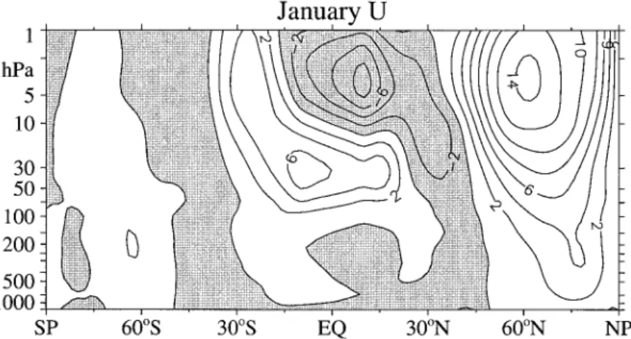
In the tropical lower stratosphere the time-averaged wind speeds are small, so the easterly minus westerly composite in Plate 2 is similar in appearance to the actual winds during the easterly phase of the QBO. At high latitudes, there is a pronounced annual cycle, with strong westerly winds during the winter season. To the north of the equator in the lower stratosphere, tropical winds alter the effective waveguide for upward and equatorward propagating planetary-scale waves (curved purple arrows). The effect of the zonal wind structure in the easterly phase of the QBO is to focus more wave activity toward the pole, where the waves converge and slow the zonal-mean flow. Thus the polar vortex north of

⬃45⬚N shows weaker westerly winds (or easterly anomaly, shown in light blue). The high-latitude wind anomalies penetrate the troposphere and provide a mechanism for the QBO to have a small influence on tropospheric weather patterns (section 6).

2.2. Temperature and Meridional Circulation

The QBO exhibits a clear signature in temperature, with pronounced signals in both tropics and extratropics.

The tropical temperature QBO is in thermal wind balance with the vertical shear of the zonal winds, expressed for the equatorial␤-planeas

⳵u

⳵z⫽⫺R H␤

⳵²T

⳵y² (1a)

[Andrews et al., 1987, equation 8.2.2], where u is the zonal wind, T is temperature, z is log-pressure height (approximately corresponding to geometric altitude),y is latitude,Ris the gas constant for dry air,H⬇ 7 km is the nominal (constant) scale height used in the log- pressure coordinates, and␤is the latitudinal derivative of the Coriolis parameter. For QBO variations centered on the equator with meridional scale L, thermal wind balance at the equator is approximated as

⳵u

⳵z⬃ R H␤

T

L². (1b)

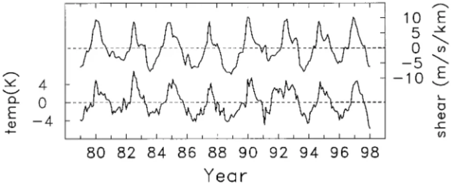
The equatorial temperature anomalies associated with the QBO in the lower stratosphere are of the order of⫾4 K, maximizing near 30–50 hPa. Figure 4 compares time series (after subtraction of the seasonal cycle) of 30-hPa temperature measurements at Singapore with the corresponding zonal wind vertical shear in the 30- to 50-hPa level, showing good correlation (see also Plate 1). The slope of ⳵u/⳵z versus temperature estimated from regression is consistent with a meridional scaleL⬃ 1000–1200 km (⬃10⬚of latitude) [Randel et al., 1999].

Smaller anomalies extend downward, with QBO variations of the order of⫾0.5 K observed near the tropopause [Angell and Korshover, 1964]. The QBO temperature anomalies also extend into the middle and upper stratosphere, where they are out of phase with the lower Figure 3. Harmonic analysis of 30-hPa zonal wind, showing

the amplitude of the annual cycle (squares), semiannual cycle (triangles), and residual deseasoned component (circles). Sym- bols show individual rawinsonde station amplitudes. Solid lines are based on binned data. Reprinted from Dunkerton and Delisi[1985] with permission from the American Meteorolog- ical Society.

184● Baldwin et al.: THE QUASI-BIENNIAL OSCILLATION 39, 2 / REVIEWS OF GEOPHYSICS

(7)

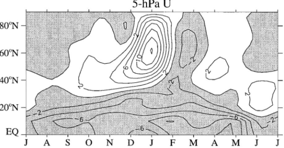
stratosphere anomalies. Figure 5 shows an example of temperature anomalies associated with an easterly phase of the QBO during NH winter 1994, derived from UK Meteorological Office (UKMO) stratospheric assimila- tion data extending to 45 km. Although these data probably underestimate the magnitude of the temperature QBO (the retrievals average over a layer deeper than the temperature anomaly), the out-of-phase vertical structure is a robust feature also observed in long time records of satellite radiance measurements [Randel et al., 1999].

Besides the equatorial maximum in QBO temperature, satellite data reveal coherent maxima over 20⬚–40⬚ latitude in each hemisphere, which are out of phase with the tropical signal. This is demonstrated in Figure 6, which shows regression of stratospheric temperatures over 13–22 km (from the microwave sounding unit chan-

nel 4) onto the 30-hPa QBO winds, for the period 1979–1999. One remarkable aspect of the extratropical temperature anomalies is that they are seasonally synchronized, occurring primarily during winter and spring in each hemisphere. Nearly identical signatures are observed in column ozone measurements (section 5), and this seasonally synchronized extratropical variability is a key and intriguing aspect of the global QBO. Because low-frequency temperature anomalies are tightly coupled with variations in the mean meridional circulation, global circulation patterns associated with the QBO are also highly asymmetric at solstice (arrows in Figure 5).

The temperature patterns in Figure 6 furthermore show signals in both polar regions, which are out of phase with the tropics, and maximize in spring in each hemisphere.

Although these polar signals are larger than the subtrop- ical maxima, and probably genuine, they are not statis- Figure 4. Equatorial temperature anomalies associated with the QBO in the 30- to 50-hPa layer (bottom

curve) and vertical wind shear (top curve).

Figure 5. Cross sections of QBO anomalies in February 1994. Temperature anomalies are contoured (⫾0.5, 1.0, 1.5 K, etc., with negative anomalies denoted by dashed contours), and components of the residual mean circulation (v៮*, w៮*) are as vectors (scaled by an arbitrary function of altitude). Reprinted fromRandel et al.

[1999] with permission from the American Meteorological Society.

(8)

tically significant in this 1979–1998 record because of large natural variability in polar regions during winter and spring.

The modulation by the QBO of zonal-mean wind (Plate 1) is coupled to modulation of the zonally averaged mean meridional circulation. The climatological circulation is characterized by large-scale ascent in the tropics, broad poleward transport in the stratosphere, and compensating sinking through the extratropical tropopause [Holton et al., 1995]. The transport of chemical trace species into, within, and out of the stratosphere is the result of both large-scale circulations and mixing processes associated with waves. Chemical processes, such as those resulting in ozone depletion, not only depend on the concentrations of trace species, but may also depend critically on temperature. Since the QBO modulates the global stratospheric circulation, including the polar regions, an understanding of the effects of the QBO not only on dynamics and temperature but also on the distribution of trace species is essential in order to understand global climate variability and change.

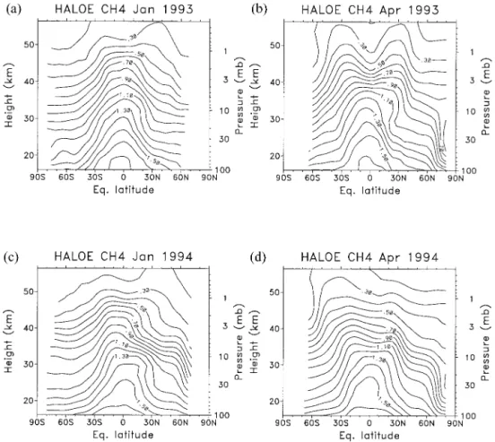
Many long-lived trace species, such as N₂O and CH₄, originate in the troposphere and are transported into the stratosphere through the tropical tropopause. Plate 3 provides a summary of the influence of the QBO on the mean meridional circulation and the transport of chemical trace species. In Plate 3 the contours illustrate schematically the isopleths of an idealized conservative, long-lived, vertically stratified tracer during the NH winter when the equatorial winds are easterly near 40 hPa (matching Plate 2). Upwelling is reflected in the broad tropical maximum in tracer density in the middle to

upper stratosphere. The extratropical anomalies caused by the QBO result in deviations from hemispheric symmetry, some of which are also due to the seasonal cycle of planetary-wave mixing.

The bold arrows in Plate 3 illustrate circulation anomalies associated with the QBO (the time-averaged circulation has been removed), which is here assumed to be easterly at 40 hPa. At the equator the QBO induces ascent (relative to the mean tropical upwelling) through the tropopause, but descent in the middle to upper stratosphere. The lower stratospheric circulation anomaly is nearly symmetric about the equator, while the circulation anomaly in the middle stratosphere is larger in the winter hemisphere (see section 5). This asymmetry is reflected in the asymmetric isopleths of the tracer. In addition to advection by the mean meridional circulation, the tracer is mixed by wave motions (approximately on isentropic, or constant potential temperature, surfac- es). This mixing is depicted by the wavy horizontal arrows. The descent from the middle stratosphere circulation anomaly creates a “staircase” pattern in the tracer isopleths between the equator and the subtropics (near 5 hPa). A second stairstep in the midlatitude winter hemisphere is formed by isentropic mixing in the region of low potential vorticity gradient which surrounds the polar vortex, known as thesurf zone[McIntyre and Palmer, 1983]. Mixing may also occur equatorward of the sub- tropical jet axis in the upper stratosphere, as illustrated by the wavy line near 3 hPa and 10⬚–20⬚N [Dunkerton and O’Sullivan, 1996]. Anomalous transport from the Southern Hemisphere (SH) to the NH near the stratopause is associated with enhanced extratropical plane- Figure 6. QBO regression using 13- to 22-km Microwave Sounding Unit temperature data for 1979–1998.

Shading denotes regions where the statistical fits are not different from zero at the 2␴level. Updated from Randel and Cobb[1994].

(9)

tary wave driving (Plate 2). The detailed effects of the QBO on tracer transport are discussed in section 5.

3. DYNAMICS OF THE QBO 3.1. QBO Mechanism

Since the QBO is approximately longitudinally symmetric [Belmont and Dartt, 1968], it is natural to try to explain it within a model that considers the dynamics of a longitudinally symmetric atmosphere. In a rotating atmosphere the temperature and wind fields are closely coupled, and correspondingly, both heating or mechanical forcing (i.e., forcing in the momentum equations) can give rise to a velocity response. Although, as noted in section 1, the current view is that mechanical forcing, provided by wave momentum fluxes, is essential for the QBO, the coupling between temperature and wind fields must be taken into account to explain many aspects of the structure.

The essence of the mechanism for the oscillation may

be demonstrated in a simple representation of the interaction of vertically propagating gravity waves with a background flow that is itself a function of height [Plumb, 1977]. Consider two discrete upward propagating internal gravity waves, forced at a lower boundary with identical amplitudes and equal but opposite zonal phase speeds. The waves are assumed to be quasi-linear (interacting with the mean flow, but not with each other), steady, hydrostatic, unaffected by rotation, and subject to linear damping. The superposition of these waves corresponds exactly to a single “standing” wave. As each wave component propagates vertically, its amplitude is diminished by damping, generating a force on the mean flow due to convergence of the vertical flux of zonal momentum. This force locally accelerates the mean flow in the direction of the dominant wave’s zonal phase propagation. The momentum flux convergence depends on the rate of upward propagation and hence on the vertical structure of zonal-mean wind. With waves of equal amplitude but opposite phase speed, zero mean flow is a possible equilibrium, but unless vertical diffu- Plate 3. Overview of tracer transport by QBO wind anomalies and mean advection. Contours illustrate

schematically the isopleths of a conservative tracer during northern winter when the QBO is in its easterly phase at 40 hPa (matching Plate 2). Tropical upwelling causes the broad maximum in tracer density in the middle to upper equatorial stratosphere, while the QBO causes deviations from hemispheric symmetry near the equator. Red arrows near the equator depict circulation anomalies of the QBO. The circulation anomaly in the equatorial lower stratosphere is approximately symmetric, while the anomaly in the upper stratosphere is much stronger in the winter hemisphere. The descent near the equator (⬃5 hPa) and ascent to the north (⬃5 hPa, 10⬚N) combine to produce a “staircase” pattern. A second stairstep is formed in midlatitudes by horizontal mixing.

(10)

sion is strong, it is an unstable equilibrium; any small deviation from zero will inevitably grow with time.

Plumb [1977] showed that the zonal-mean wind anomalies descend in time, as illustrated in Figure 7.

Each wave propagates vertically until its group velocity is slowed, and the wave is damped as it encounters a shear zone where兩u៮ ⫺ c兩 is small (u៮ is the zonal-mean wind andcis the zonal phase speed of the wave). As the shear zone descends (Figure 7a) the layer of eastward winds becomes sufficiently narrow that viscous diffusion de- stroys the low-level eastward winds. This leaves the eastward wave free to propagate to high levels through westward mean flow (Figure 7b), where dissipation and the resulting eastward acceleration gradually build a new eastward regime that propagates downward (Figures 7c and 7d).

The process just described repeats, but with westerly shear descending above easterly shear, leading to the formation of a low-level easterly jet. When the easterly jet decays, the westward wave escapes to upper levels, and a new easterly shear zone forms aloft. The entire sequence, as described, represents one cycle of a non- linear oscillation. The period of the oscillation is determined, among other things, by the eastward and westward momentum flux input at the lower boundary and by the amount of atmospheric mass affected by the waves.

InPlumb’s [1977]Boussinesq formulation the QBO pe-

riod is inversely proportional to momentum flux. The same is true in a quasi-compressible atmosphere, but the decrease in atmospheric density with height results in a substantially shorter period.

Simple representations such as Plumb’s capture the essential wave mean-flow interaction mechanism leading the QBO. However, they cannot explain why the QBO is an equatorial phenomenon (notwithstanding its important links to the extratropics). One reason the QBO is equatorially confined may be that it is driven by equatorially trapped waves. However, it is also possible that the QBO is driven by additional waves and is confined near the equator for another, more fundamental, reason.

Some simple insights on this point come from considering the equations for the evolution of a longitudinally symmetric atmosphere subject to mechanical forcing. A suitable set of model equations for such a longitudinally symmetric atmosphere is as follows:

⳵u

⳵t ⫺2⍀sin␾v⫽F (2) 2⍀sin␾⳵u

⳵z⫹ R aH

⳵T

⳵␾⫽0 (3)

⳵T

⳵t ⫹wHN²

R ⫽⫺␣T (4)

1 acos␾

⳵

⳵␾v cos␾⫹ 1

␳0

⳵

⳵z共␳0w兲⫽0 (5) Here ␾ is latitude, ⍀ is the angular frequency of the Earth’s rotation,ais the radius of the Earth, and␳0is a nominal basic state density proportional to exp (⫺z/H).

In (4), N² is the square of the buoyancy frequency (a measure of static stability), defined as

N²⬅R

H冉^dT^dz⁰^⫹^␬T^H⁰冊^,

whereT₀ is a reference temperature profile depending only onzand␬ ⫽ R/c_p, wherec_pis the specific heat of air at constant pressure. Finally, u is the longitudinal component of wind,Tis the temperature deviation from T₀, andv andw are the latitudinal and vertical components, respectively, of velocity.

Equation (2) states that the longitudinal acceleration is equal to the applied force F (here assumed to be a given function of latitude, height, and time), plus the Coriolis force associated with the latitudinal velocity.

The Coriolis force is the important effect of rotation; the response to an applied force is not simply an equivalent acceleration. Instead, part of the applied force is balanced by a Coriolis force; how much depends on how large a latitudinal velocity is excited. Equation (3) is the thermal wind equation coupling the longitudinal velocity field and the temperature field, which follows from the assumption that the flow is in hydrostatic and geostro- phic balance. Equation (4) states that the rate of change of temperature is equal to the diabatic heating plus the Figure 7. Schematic representation of the evolution of the

mean flow inPlumb’s [1984] analog of the QBO. Four stages of a half cycle are shown. Double arrows show wave-driven acceleration, and single arrows show viscously driven accelera- tions. Wavy lines indicate relative penetration of eastward and westward waves. AfterPlumb[1984]. Reprinted with permission.

(11)

adiabatic temperature change associated with vertical motion. Here the diabatic heating is represented by the term ⫺␣T, where ␣ is a constant rate, representing long-wave heating or cooling. Equation (5) is the mass- continuity equation.

Equation (2)–(5) may be regarded as predictive equations for the unknowns⳵u/⳵t,⳵T/⳵t,v, andw. They may be combined to give a single equation for one of the unknowns, with a single forcing term containing the force F. It is convenient to follow Garcia [1987] and assume that the time dependence is purely harmonic.

Thus we writeF(␾,z,t)⫽Re (Fˆ(␾,z)e^i␻t) and consider the response in the longitudinal velocityu, assumed to be of the formu(␾,z,t)⫽ Re (uˆ(␾,z)e^i␻t). Equations (2)–(5) then can be transformed to a single equation

1 cos␾

⳵

⳵␾ 冉^cos¹^␾^⳵␾^⳵ 冉^cos^sin^␾^␾^uˆ冊冊

⫹ 1

␳0

⳵

⳵z冉^␳⁰冉¹^⫹î␻^␣冊 ⁴^⍀^N²²â²^cos^sin^␾^␾^⳵^⳵zûˆ冊

⫽ 1 i␻

1 cos␾

⳵

⳵␾ 冉^cos¹^␾^⳵␾^⳵ 冉^cos^sin^␾^␾^Fˆ冊冊^{. (6)}

The operator acting onuˆon the left-hand side of the equation is elliptic, consistent with the well-known prop- erty of rotating, stratified systems that localized forcing gives rise to a nonlocal response. For an oscillation with period 2 years, ␻ ⬇ 10^⫺7 s^⫺1. The Newtonian cooling rate ␣is, for the lower stratosphere, generally taken to be about 5⫻10^⫺7s^⫺1, corresponding to a timescale of about 20 days. Hence the factor 1⫹ ␣/(i␻) appearing in the second term on the left-hand side may be approximated by␣/(i␻).

A scale analysis of (6) shows that when rotational effects are weak, i.e., when sin␾is small, the dominant balance is between the forcing term and the first term on the left-hand side. This implies that the acceleration is equal to the applied force. More generally, the second term on the left-hand side will play a major role in the balance, implying that the Coriolis force must be substantially canceling the applied force in (2). Following Haynes [1998], a quantitative comparison of the two terms on the left-hand side of (6) may be performed by assuming a height scaleD and a latitudinal scaleL for the velocity response. Then, at low latitudes, noting that sin ␾ scales as ␾ and hence as L/a, the ratio of the second term on the left-hand side of (6) to the first is 4⍀²L⁴␣/(a²D²N²␻). It follows that if L ⬍⬍ (aDN/

(2⍀))^{1/ 2}(␻/␣)^1/4, then the acceleration is approximately equal to the applied force. This might be called the “tropical response”; it occurs if the latitudinal scale L is small enough. On the other hand, ifL ⬎⬎ (aDN/

(2⍀))^{1/ 2}(␻/␣)^1/4, then the applied force is largely canceled by the Coriolis torque and most of the response to the applied force appears as a mean meridional circulation. This might be called the “extratropical response”

(though clearly the scaling would require modification if it were to be applied well away from the equator).

The physical reason for the distinction between the tropical and extratropical responses is the link between velocity and temperature fields in a rotating system, expressed by (3), together with the temperature damping implied by (4). At high latitudes an applied force, varying on sufficiently long timescales, will tend to be canceled by the Coriolis force due to a mean meridional circulation. This circulation will induce temperature anomalies, upon which the thermal damping will act, effectively damping the velocity response and limiting its amplitude. At low latitudes, on the other hand, the force will give rise to an acceleration, there will be relatively little temperature response, and thermal damping will have little effect on the velocity response. It is as if low-latitude velocities have a longer “memory” than high-latitude velocities; anomalies at low latitudes take longer to dissipate [Scott and Haynes, 1998]. Thus the QBO mechanism might be expected to work only at low latitudes. TheLindzen and Holton[1968] experiments in a 2-D model showed that the Coriolis torque reduced the amplitude of the wind oscillation away from the equator.Haynes[1998] went further to suggest that the transition from the tropical regime to the extratropical regime may set the latitudinal width of the QBO, rather than, for example, the latitudinal scale of the waves that provide the necessary momentum flux. Simulations in a simple numerical model where the momentum forcing is provided by a latitudinally broad field of small-scale gravity waves, designed not to impose any latitudinal scale, predicted a transition scale at about 10⬚.

To summarize, a long-period oscillation that requires the zonal velocity field to respond directly to a wave- induced forced is likely to work only in the tropics, since elsewhere the force will tend to be balanced by the Coriolis torque due to a meridional circulation. For this reason, 1-D models, which omit Coriolis torques alto- gether, can capture the tropical oscillation. However, they cannot simulate the latitudinal structure that arises in part from the increase of Coriolis torques with latitude.

3.2. Waves in the Tropical Lower Stratosphere There exists a broad spectrum of waves in the tropics, many of which contribute to the QBO. On the basis of observations of wave amplitudes, we now believe that a combination of Kelvin, Rossby-gravity, inertia-gravity, and smaller-scale gravity waves provide most of the momentum flux needed to drive the QBO [Dunkerton, 1997]. All of these waves originate in the tropical troposphere and propagate vertically to interact with the QBO. Convection plays a significant role in the genera- tion of tropical waves. Modes are formed through lateral propagation, refraction, and reflection within an equatorial waveguide, the horizontal extent of which depends on wave properties, for example, turning points where

(12)

wave intrinsic frequency equals the local inertial frequency.

Equatorward propagating waves originating outside the tropics, such as planetary Rossby waves from the winter hemisphere, may have some influence in upper levels of the QBO [Ortland, 1997]. The lower region of the QBO (⬃20–23 km) near the equator is relatively well shielded from the intrusion of extratropical planetary waves [O’Sullivan, 1997].

Vertically propagating waves relevant to the QBO are either those with slow vertical group propagation under- going absorption (due to radiative or mechanical damping) at such a rate that their momentum is deposited at QBO altitudes, or those with fast vertical group propagation up to a critical level lying within the range of QBO wind speeds [Dunkerton, 1997]. The height at which momentum is deposited depends on the vertical group velocity (supposing for argument’s sake that the damping rate per unit time is independent of wave properties). Waves with very slow group propagation are confined within a few kilometers of the tropopause [Li et al., 1997]. On the other hand, waves with fast vertical group velocity and with phase speeds lying outside the range of QBO wind speeds propagate more or less transparently through the QBO.

Long-period waves tend to dominate spectra of horizontal wind and temperature. However, higher-frequency waves contribute more to momentum fluxes than might be expected from consideration of temperature alone. We can organize the waves relevant to the QBO into three categories: (1) Kelvin and Rossby-gravity waves, which are equatorially trapped; periods of ⲏ3 days; wave numbers 1–4 (zonal wavelengths ⲏ10,000 km); (2) inertia-gravity waves, which may or may not be equatorially trapped; periods of⬃1–3 days; wave numbers⬃4–40 (zonal wavelengths⬃1000–10,000 km); and (3) gravity waves; periods ofⱗ1 day; wave number⬎40 (zonal wavelengths ⬃10–1000 km) propagating rapidly in the vertical. (Waves with very short horizontal wave- lengthsⱗ10 km tend to be trapped vertically at tropospheric levels near the altitude where they are forced and are not believed to play a significant role in middle atmosphere dynamics.)

The observations reviewed below suggest that intermediate and high-frequency waves help to drive the QBO. However, uncertainties remain in the wave momentum flux spectrum, with regard to actual values of flux and the relative contribution from various parts of the spectrum. Although the momentum flux in mesoscale waves is locally very large, it is necessary to know the spatial and temporal distribution of these waves in order to assess their role in the QBO. Available observations are insufficient for this purpose. For intermediate-scale waves, it is unclear what fraction of the waves is important to the QBO without a more precise estimate of their phase speeds, modal structure, and absorption characteristics. Twice-daily rawinsondes provide an accurate picture of vertical structure but have poor hor-

izontal and temporal coverage. Their description of horizontal structure is inadequate, and temporal aliasing may occur, obscuring the true frequency of the waves.

The QBO, in principle, depends on wave driving from the entire tropical belt, but the observing network can only sample a small fraction of horizontal area and time.

Thus it is uncertain how to translate the information from local observations of intermediate and small-scale waves into a useful estimate of QBO wave driving on a global scale. Ultimately, satellite observations will provide the needed coverage in space and time. These observations have already proven useful for planetary- scale equatorial waves and small-scale extratropical gravity waves with deep vertical wavelength. Significant improvement in the vertical resolution of satellite instruments and their ability to measure or infer horizontal wind components will be necessary, however, before such observations are quantitatively useful for estimates of momentum flux due to intermediate and small-scale waves in the QBO region.

3.2.1. Kelvin and Rossby-gravity waves. Kelvin and Rossby-gravity waves were detected using rawinsonde observational data byYanai and Maruyama[1966]

andWallace and Kousky[1968b]; these discoveries were important to the development of a modified theory of the QBO byHolton and Lindzen[1972]. For reviews of early equatorial wave observations, see Wallace[1973], Holton[1975],Cornish and Larsen[1985],Andrews et al.

[1987], and Dunkerton[1997]. Interpretation of distur- bances as equatorial wave modes relies on a comparison of wave parameters (e.g., the relation of horizontal scale and frequency), latitudinal structure (e.g., symmetric or antisymmetric about the equator), and phase relation- ship between variables (e.g., wind components and temperature) with those predicted by theory. The identifi- cation of equatorial modes is relatively easy in regions with good spatial coverage so that coherent propagation may be observed.

Long records of rawinsonde data from high-quality stations have been used to derive seasonal and QBO- related variations of Kelvin and Rossby-gravity wave activity near the equator [Maruyama, 1991; Dunkerton, 1991b, 1993;Shiotani and Horinouchi, 1993;Sato et al., 1994; Wikle et al., 1997]. The QBO variation of Kelvin wave activity observed in fluctuations of zonal wind and temperature is consistent with the expected amplifica- tion of these waves in descending westerly shear zones.

Annual variation of Rossby-gravity wave activity is observed in the lowermost equatorial stratosphere and may help to explain the observed seasonal variation of QBO onsets near 50 hPa [Dunkerton, 1990].

Equatorially trapped waves have been observed in temperature and trace constituent data obtained from various satellite instruments. Most of these studies dealt with waves in the upper stratosphere relevant to the stratopause semiannual oscillation (SAO); a few, however, also observed waves in the equatorial lower stratosphere relevant to the QBO [e.g., Salby et al., 1984;

(13)

Randel, 1990;Ziemke and Stanford, 1994;Canziani et al., 1995;Kawamoto et al., 1997;Shiotani et al., 1997;Mote et al., 1998; Canziani and Holton, 1998]. It is difficult to detect the weak, shallow temperature signals associated with vertically propagating equatorial waves, and satellite sampling usually recovers only the lowest zonal wave numbers (e.g., waves 1–6). Nevertheless, satellite observations are valuable for their global view, complement- ing the irregular sampling of the rawinsonde network.

Two-dimensional modeling studies [Gray and Pyle, 1989; Dunkerton, 1991a, 1997] showed that Kelvin and Rossby-gravity waves are insufficient to account for the required vertical flux of momentum to drive the QBO.

The required momentum flux is much larger than was previously assumed because the tropical stratospheric air moves upward with the Brewer-Dobson circulation.

When realistic equatorial upwelling is included in models, the required total wave flux for a realistic QBO is 2–4 times as large as that of the observed large-scale, long-period Kelvin and Rossby-gravity waves. Three- dimensional simulations [e.g., Takahashi and Boville, 1992; Hayashi and Golder, 1994; Takahashi, 1996] de- scribed in section 3.3.2 confirm the need for additional wave fluxes. Therefore it is necessary to understand better from observations the morphology of smaller- scale inertia-gravity and gravity waves and their possible role in the QBO.

3.2.2. Inertia-gravity waves. Eastward propagating equatorial inertia-gravity waves are seen in westerly shear phases of the QBO, while westward propagating waves are seen in easterly shear phases. Observational campaigns using rawinsondes have provided data with high temporal and vertical resolution, so that analysis is possible both for temporal and vertical phase variations.

Cadet and Teitelbaum[1979] conducted a pioneering study on inertia-gravity waves in the equatorial region, analyzing 3-hourly rawinsonde data at 8.5⬚N, 23.5⬚W during the Global Atmospheric Research Project Atlan- tic Tropical Experiment (GATE). The QBO was in an easterly shear phase. They detected a short vertical wavelength (⬍1.5 km) inertia-gravity wave-like structure having a period of 30–40 hours. The zonal phase velocity was estimated to be westward.

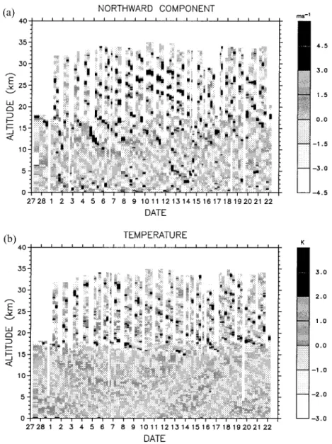
Tsuda et al. [1994a, 1994b] conducted an observa- tional campaign focusing on waves in the lower stratosphere at Watukosek, Indonesia (7.6⬚S, 112.7⬚E), for 24 days in February–March 1990 when the QBO was in a westerly shear phase. Wind and temperature data were obtained with a temporal interval of 6 hours and vertical resolution of 150 m. Figure 8 shows a time-height section of temperature fluctuations with periods shorter than 4 days. Clear downward phase propagation is observed in the lower stratosphere (above about 16 km altitude).

The vertical wavelength is about 3 km, and the wave period is about 2 days. Similar wave structure was seen also for zonal (u) and meridional wind (v) fluctuations.

The amplitudes of horizontal wind and temperature fluctuations were about 3 m s^⫺1and 2 K, respectively.

On the basis of hodographic analysis, assuming that these fluctuations are due to plane inertia-gravity waves, Tsuda et al. [1994b] showed that most wave activity propagated eastward and upward in the lower stratosphere. Similar characteristics were observed in their second campaign, in Bandung, Indonesia (107.6⬚E, 6.9⬚S), during another westerly shear phase of the QBO (November 1992 to April 1993) [Shimizu and Tsuda, 1997].

Statistical studies of equatorial inertia-gravity waves have been made using operational rawinsonde data at Singapore (1.4⬚N, 104.0⬚E). Maruyama[1994] andSato et al. [1994] analyzed the year-to-year variation of 1- to 3-day wave activity in the lower stratosphere using data from Singapore spanning 10 years. Extraction of waves by their periods is useful since the ground-based wave frequency is invariant during the wave propagation in a steady background field. The QBO can be considered sufficiently steady for these purposes for inertia-gravity waves having periods shorter than several days.

Maruyama [1994] analyzed the covariance of zonal wind and the time derivative of temperature for 1- to 3-day components and estimated the vertical flux of zonal momentum per unit densityu⬘w⬘using the following relation derived from the thermodynamic equation for adiabatic motions:

⳵T⬘

⳵t u⬘⫽⫺冋^T^៮^g^N²册 ^c^{cˆ u}^⬘^w^⬘^, ⁽⁷⁾

whereT is temperature,tis time,uandware the zonal and vertical components of wind velocity, c is the ground-based horizontal phase speed,cˆ ⫽ c⫺ u៮ is the intrinsic horizontal phase speed, u៮ is the background wind speed, and the overbar indicates a time average.

Sincecˆis not obtained from the observational data, this estimate is possible only when u៮ is small enough to assumecˆ/c⬃1. Maruyama showed that the momentum flux u⬘w⬘ is largely positive and that the magnitude is comparable to that of long-period Kelvin waves in the westerly shear phase of the QBO.

Sato et al. [1994] examined the interannual variation of power and cross spectra of horizontal wind and temperature fluctuations in the period range of 1–20 days at Singapore. They found that spectral amplitudes are maximized around the tropopause for all components in the whole frequency band, although the altitudes of the tropopause maxima are slightly different. TheT andu spectra are maximized around a 10-day period, corresponding to Kelvin waves. In the lower stratosphere the wave period shortens, for example, 9 days at 20 km to 6 days at 30 km. On the other hand, v spectra are maximized around 5 days, slightly below the tropopause, corresponding to Rossby-gravity waves. The Rossby- gravity wave period also becomes shorter with increasing altitude in the lower stratosphere, consistent with the analysis ofDunkerton[1993] based on rawinsonde data at several locations over the tropical Pacific. An impor-

(14)

tant fact is that spectral amplitudes are as large at periods shorter than 2–3 days as for long-period Kelvin waves and Rossby-gravity waves.

The activity of inertia-gravity and Kelvin waves is observed to be synchronized with the QBO. Plate 4 shows power and cross spectra as a function of time averaged over the height region 20–25 km in the lower stratosphere. A low-pass filter with cutoff of 6 months was applied in order to display the relation with the QBO more clearly. Dominant peaks in the power spectra of T andu are observed in the 1- to 3-day period range during both phases of the QBO and around the 10-day period in the westerly shear phase of the QBO.

The latter peak corresponds to Kelvin waves.

The quadrature spectra Q_Tu(␻) correspond to the covariance of zonal wind and time derivative of temperature. Thus large negative values observed around a 10-day period in the westerly shear phase show the positive u⬘w⬘ associated with Kelvin waves [Maruyama,

1991, 1994]. Such a tendency is not clear at shorter periods in the quadrature spectra. Clear synchronization with the QBO is seen in the cospectra C_Tu(␻) in the whole range of frequencies. Positive and negative values appear in the westerly and easterly shear phases, respectively, though the negative values are weak around the 10-day period. This feature cannot be explained by the classical theory of equatorial waves in a uniform background wind [Matsuno, 1966], which predicts that the covariance of T and u should be essentially zero.

Dunkerton[1995] analyzed theoretically and numeri- cally the covariance ofT andu for 2-D (plane) inertia- gravity waves in a background wind having vertical shear and derived the following relation:

T⬘u⬘⫽冋^2gk兩cˆ兩^T^៮^N 册^u^៮^z^{兩u⬘w⬘兩} ⁽⁸⁾

Figure 8. A time-height section of short-period (⬍4 days) (a) northward velocity component and (b) temperature, at Watukosek, Indonesia (7.6⬚S, 112.7⬚E), for 24 days in February to March 1990. FromTsuda et al. [1994b].

(15)

Plate 4. Power spectra for (a)T and (b)u fluctuations at Singapore as a function of time, averaged over 20–25 km. Contour interval 0.5 K², and 2 (m s^⫺1)², respectively. (c) Cospectra and (d) quadrature spectra of Tanducomponents. Contour interval 0.5 K (m s^⫺1). Red and blue colors show positive and negative values, respectively. The bold solid line represents a QBO reference time series. AfterSato et al.[1994].

(16)

for slowly varying, steady, conservative, incompressible waves. This theory was extended to 3-D equatorially trapped waves (T. J. Dunkerton, manuscript in prepara- tion, 2001). According to (8), the covariance is proportional to the vertical shear and vertical flux of horizontal momentum, or radiation stress. The sign of the covariance is determined by the vertical shear, independent of the horizontal and vertical direction of inertia-gravity wave propagation. This is qualitatively consistent with the observation in Plate 4c.

Sato and Dunkerton [1997] estimated momentum fluxes associated with 1- to 3-day period waves directly and indirectly based on the quadrature and cospectra of Tanducomponents at Singapore obtained bySato et al.

[1994]. Unlike Kelvin waves, which propagate only eastward, inertia-gravity waves can propagate both eastward and westward. Thus the net momentum flux estimate from quadrature spectra as obtained by Maruyama [1994] may be a residual after cancelation between positive and negative values. On the other hand, cospectra correspond to the sum of absolute values of positive and negative momentum fluxes. Using an indirect estimate of momentum fluxes from cospectra and a direct estimate from quadrature spectra, positive and negative parts of momentum fluxes can be obtained separately.

The direct estimate of momentum flux for Kelvin

waves (5- to 20-day period) is 2–9 ⫻ 10^⫺3 m² s^⫺2and accords with the indirect estimate within the estimation error, supporting the validity of the indirect method.

Note that momentum flux is properly measured in pas- cals (Pa), equal to air density times the product of velocity components. In most QBO literature the density term is ignored, and the resulting “flux” is described in units of m²s^⫺2. Near the tropical tropopause the density is about 0.1 in MKS units, providing an easy conversion between the two definitions of flux.

The result for 1- to 3-day periods is shown in Figure 9, assuming plane inertia-gravity waves. The indirect estimate of momentum flux for 1- to 3-day-period components in westerly shear is 20–60⫻10^⫺3m²s^⫺2, while the direct estimate is only 0–4 ⫻ 10^⫺3 m² s^⫺2. For easterly shear, the indirect estimate is 10–30⫻10^⫺3m² s^⫺2, while the direct estimate is almost zero. The dis- crepancy between the indirect and direct estimates indicates a large cancelation between positive and negative momentum fluxes.

There is ambiguity in the indirect estimate according to the assumed wave structure. If equatorially trapped modes are assumed, the values should be reduced by 30–70%. On the other hand, if there is aliasing from higher-frequency waves (with periods shorter than 1 day, for twice-daily data such as rawinsonde data at Singa- Figure 9. Momentum flux estimates for short-period (1–3 days) component in the (a) westerly and (b)

easterly shear phases. Left panels show indirect estimates corresponding to a sum of absolute values of positive and negative momentum fluxes. Right panels show direct estimates corresponding to net momentum fluxes.

FromSato and Dunkerton[1997].