Analysis of the Equatorial Lower Stratosphere Quasi-Biennial Oscillation (QBO) UsingECMWF-Interim Reanalysis Data Set

(1)

This content has been downloaded from IOPscience. Please scroll down to see the full text.

Download details:

IP Address: 134.245.215.185

This content was downloaded on 11/03/2016 at 14:03

Please note that terms and conditions apply.

Analysis of the Equatorial Lower Stratosphere Quasi-Biennial Oscillation (QBO) Using ECMWF-Interim Reanalysis Data Set

View the table of contents for this issue, or go to the journal homepage for more 2016 IOP Conf. Ser.: Earth Environ. Sci. 31 012032

(http://iopscience.iop.org/1755-1315/31/1/012032)

Home Search Collections Journals About Contact us My IOPscience

(2)

Analysis of the Equatorial Lower Stratosphere Quasi-Biennial Oscillation (QBO) Using ECMWF-Interim Reanalysis Data Set

Givo Alsepan¹*, Sandro Wellyanto Lubis², Sonni Setiawan¹

1 Department of Geophysics and Meteorology, Bogor Agricultural University (IPB), Indonesia

2 Physics of the Atmosphere, GEOMAR Helmoltz Centre for Ocean Research Kiel, Germany

E-mail: givoalsepan@yahoo.com

Abstract. The ERA-Interim data set from Europe Center for Medium Range Weather Forecasting (ECMWF) was used to quantitatively analyze the characteristic of equatorial quasi-biennial oscillation (QBO). Analysis of spatial and temporal of the data showed that the zonally symmetric easterly and westerly phase of QBO regimes alternate with period of ~27.7 months. Based on Equivalent QBO Amplitude (EQA) method, the maximum amplitudes in zonal mean zonal wind (u), temperature (T), vertical shear (du/dz) and quadratic vertical shear (d²u/dz²) are ~28.3 m/s , ~3.4 K, ~4.8 m/s/km, and ~1.0 m/s/km² respectively. The amplitudes decay exponentially with a Gaussian distribution in latitude. The twofold-structure of QBO descends downward at rate of ~1 km/month. The temperature anomaly can be used to analyze the characteristic of QBO which satisfies the thermal wind balance relation in the lower- stratosphere due to very small contribution of the mean meridional and vertical motion.

Moreover, the concentration of the total column ozone (TCO) in the tropics is significantly influenced by QBO. During the westerly phase of QBO, the TCO is relatively increased in the lower-stratosphere, but decreased during the opposite phase.

1. Introduction

The stratospheric region in the equator is dominated by descending downward of westerly and easterly wind which was first introduced by Ebdon (1960) and Reed et al (1961), and then it was called as Quasi-Biennial Oscillation (Angell and Korshover 1964). QBO is an oscillation of westerly and easterly wind descending downward in the lower-stratosphere of the equatorial region (~16 – 50 km) with period of 28 months in average (Baldwin et al 2001). The easterly phase of QBO has greater maximum amplitude than the westerly phase, and the amplitudes have symmetrical pattern in the equator with a Gaussian distribution (Baldwin et al 2001; Pascoe et al 2005).

Mechanism of QBO was first shown by Holton and Lindzen (1972), where QBO is a result of the interaction between mean flow and the equatorial planetary waves. Holton and Lindzen were the first

*Corresponding author

ISS-CNS IOP Publishing

IOP Conf. Series: Earth and Environmental Science 31 (2016) 012032 doi:10.1088/1755-1315/31/1/012032

(3)

people who conducted the modeling of QBO based on the propagation of Kelvin waves and Rosby- gravity waves. Holton (2004) explained that QBO is only occurred in the equator because Kelvin waves and Rosby-gravity waves are only formed in a region around 12⁰ N – 12⁰ S. The equatorial region provides a great energy originated from releasing of laten heat in macro scale of convective clouds for creating the planetary equatorial waves and forcing them to the lower-stratosphere. QBO is not occurred in high latitude regions because there is no enough energy to force the equatorial planetary waves to the lower-stratosphere, although there is a formation of clouds and “front” area in high latitude.

In addition to discuss about zonal wind oscillation, QBO also influences the chemical and physical process in the lower-stratosphere. Holton (2004) has proved that QBO satisfies the thermal wind equation if wind shear of zonal wind is associated with temperature in the lower-stratosphere.

Meanwhile, Baldwin et al (2001) showed that temperature and ozone data sets can be used to analyze QBO.

This study uses ERA-Interim data sets from ECMWF (Europe Center for Medium Range Weather Forecasting). ERA-Interim is the last atmospheric reanalysis data sets produced by ECMWF after ERA-40. These data sets are available from January 1979 to present and has the pressure levels from 1000 to 1 hPa (Dee et al 2011).

The aims of this study are to quantify the characteristics of QBO (period, oscillation amplitude, propagation rate, Gaussian distribution of amplitude), to prove the thermal wind equation, and to show the relationship between QBO and total column ozone (TCO) using zonal wind, temperature, and TCO data sets obtained from ECMWF-Interim Reanalysis.

2. Methods

ERA-Interim data sets from ECMWF (Europe Center for Medium Range Weather Forecasting) during 30 years (January 1981 to December 2010) were used in this study, and the spatial resolution of the data is 220 km x 220 km. The data are monthly data sets from 1 hPa (~49 km) to 1000 hPa consisting of zonal wind (u), temperature (T), and total colum ozone (TCO). Temperature and zonal wind data sets are used to quantify QBO and to analyze the thermal wind balance relation, and total column ozone data sets are used to analyzed the relationship of QBO and the fluctuation of ozone in the lower- stratosphere.

2.1.Equivalent QBO Amplitude (EQA)

EQA was first introduced by Randel et al (2004). This method is developed to calculate the amplitude of QBO by determining the standard deviation of zonal wind anomaly, then the standard deviation is multiplied by 2. The mathematical formula can be formulated as follows:

(1) EQA method can also be used to investigate the characteristic of QBO using other parameters such as temperature, wind shear, and quadratic vertical shear.

2.2.Spectral Analysis

Spectral analysis is used to calculate a hidden period or to estimate a spectral density of time series data. This method is a modification of Fourier analysis. Fourier analysis can be represented by using Fourier series, where every periodic function can be represented by unlimited sum of sine and cosine function. Mathematical function of Fourier series can be formulated as follows:

anomaly 2 EQA=s

(4)

0 1

( ) cos sin

2 _i ⁿ 1 ⁿ 1

a n t n t

f t ^∞ a

π

b

π

=

 

= +  + 

 

∑

1

1 ( ) cos d

1 1

n

a f t n t

π

t

−

=

∫

1

1 ( ) sin d

1 1

n

b f t n t

π

t

−

=

∫

⁽²⁾

Spectrum f( )ω is a Fourier transformation of autocovariance function which can be formulated as follows:

(3)

2.3.Cross-Correlation

Cross-correlation is used to explain an association between two non-linear randomly variables. In analysis of time series, cross-correlation between two time series data describes cross-correlation coefficient r_xy( )k which is calculated by using a simple formula of Box and Jenkins (1976) as follows:

(4)

Where k is a lag with k = ± ±0, 1, 2,....,n and s s_{x y} is a standard deviation of series x and y respectively. Meanwhile, c_xy( )k is a cross-covariance function at lag k( ) which can be obtained from:

(5) Where x and y are the average of respective variables and t is time. Cross-correlation is generally used to determine lag value of two non-liniear time series data.

3.Results

3.1.Characteristics of QBO

Time-height section of monthly zonal mean zonal wind from ERA-Interim data sets during 1981 to 2010 was shown in Figure 1, and the result is appropriate with the time-height section found by Naujokat (1986) using radiosonde data sets and Gray et al (2001b) using rokcetsonde data sets.

Oscillation of westerly and easterly zonal wind is dominantly occurred in the lower-stratosphere about

~100 – 5 hPa (~16 – 35 km), meanwhile the atmospheric layer above 5 hPa is dominated by Semiannual Oscillation (SAO) which is appropriate with the result of Pascoe et al (2005). Generally, easterly zonal wind is stronger than westerly zonal wind.

( ) 1 ( ) exp ^{i k}

k

f ω γ k ^ω

π

∞ −

=−∞

=

∑

( ) ^xy( )

xy

x y

c k r k

= s s

( ) 1 ( )( ); 1; 1; 0

xy t t k

c k x x y y t N k

N ⁺

=

∑

− − = − ≥

(5)

Figure 1. Monthly zonal mean zonal wind using ERA-Interim data sets (1981 to 2010) in a function of time and pressure. Blue color indicates easterly zonal wind and red color indicates westerly zonal wind.

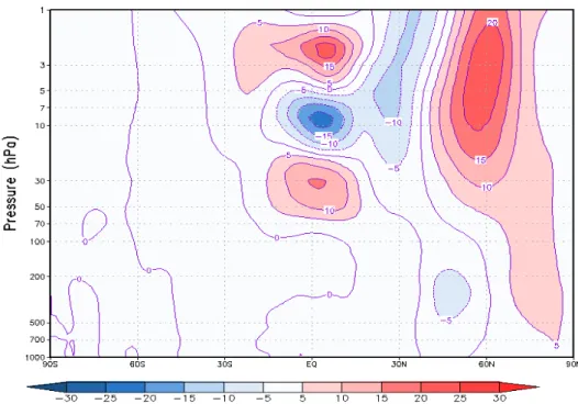
Figure 2. Latitude-height section of zonal mean zonal wind anomaly based on ERA-Interim data sets in January 1981. Blue color indicates easterly zonal wind and red color indicates westerly zonal wind.

(6)

E a) W

E b) W Figure 3. Meridional structure of zonal mean zonal wind. a) at 30 hPa, b) at 100 hPa.

(7)

Figure 2 is latitude-height section of zonal mean zonal wind in January 1981 which shows the threefold-structure. The easterly phase (E) is above the westerly phase (W) of zonal wind at ~100 – 5 hPa in the equator, so it is called as the twofold-structure of QBO. Another structure above ~5 hPa in the upper-stratosphere is indicated as SAO. The structures are symmetry in latitude, where the amplitude is increased in the equator and decreased in the high latitude.

Based on time-latitude section in Figure 3, oscillation of zonal wind is clearly occurred at ~30 hPa (Figure 3a) compared with a level at ~100 hPa (Figure 3b) in the equator. Oscillation of westerly and easterly zonal wind at ~100 hPa can not be seen clearly, so it indicates that oscillation of QBO is stronger at ~30 hPa than at ~100 hPa. In Figure 3, we can also see that oscillation of QBO ascends in the equator and descends in the higher latitude.

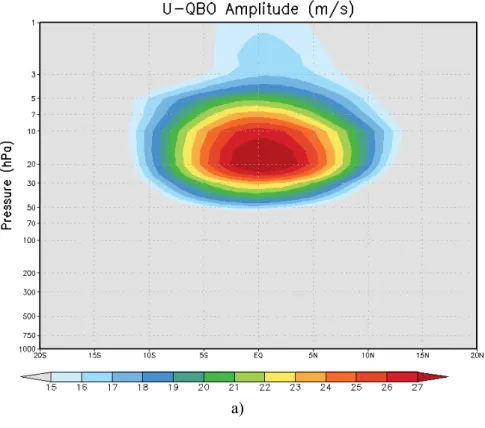
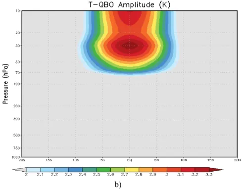
Figure 4a shows that the maximum amplitude of QBO is at ~20 hPa (~27 km) above the surface of equatorial region with the value of ~28.3 m/s where QBO dominates the variability of zonal wind. In the other side, the maximum amplitude of QBO in temperature is occurred at ~30 hPa (~25 km) above the surface with the value of ~3.4 K (Figure 4b). The amplitudes of zonal wind and temperature are increased in the equator, but they are exponentially decreased with a Gaussian distribution in latitude (Figure 5). Those conditions indicate that QBO is only occurred in the equatorial area. According to Holton (2004), QBO is only strongly formed in the area around 12⁰ N – 12⁰ S.

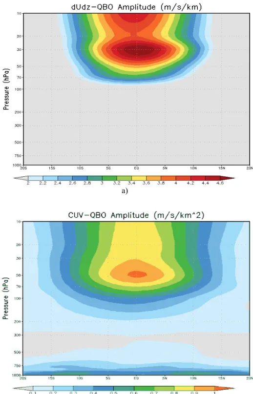
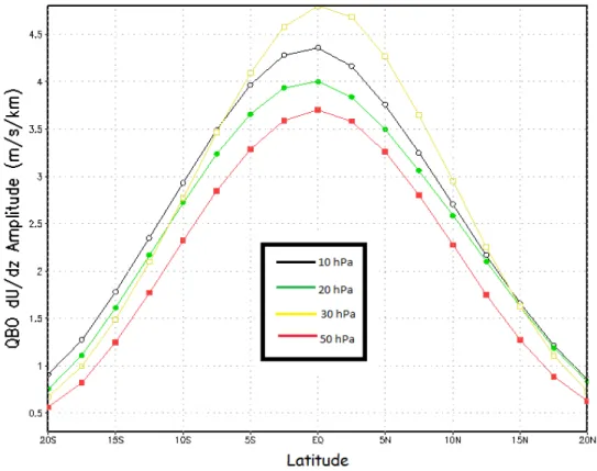
Derivative of zonal wind can also be used to analyze the structure of QBO. Wind shear (du/dz) is the first derivative of zonal wind. The result shows that QBO in the lower-stratosphere with the maximum amplitude of ~4.8 m/s/km is occurred at ~30 hPa (~25 km) above the surface (Figure 6a). Second derivative of zonal wind is a quadratic vertical shear (d²u/dz²) which shows that the maximum amplitude of QBO is occurred at ~50 hPa (~21 km) above the surface with the value of ~1.0 m/s/km² (Figure 6b). The amplitudes of QBO in wind shear and quadratic vertical shear are increased in the equator, but they are exponentially decreased with a Gaussian distribution in latitute (Figure 7).

a)

(8)

b)

Figure 4. Amplitudes of QBO using EQA method. a) U-QBO amplitude, b) T-QBO amplitude.

Figure 5. Meridional profile of U-QBO with a Gaussian distribution.

(9)

a)

b)

Figure 6. Amplitudes of QBO using EQA method in first derivative (dU/dz) and second derivative (d²U/dz²) of zonal wind. a) dU/dz-QBO amplitude, b) d²U/dz²-QBO amplitude.

(10)

Figure 7. Meridional profile of dU/dz-QBO with a Gaussian distribution.

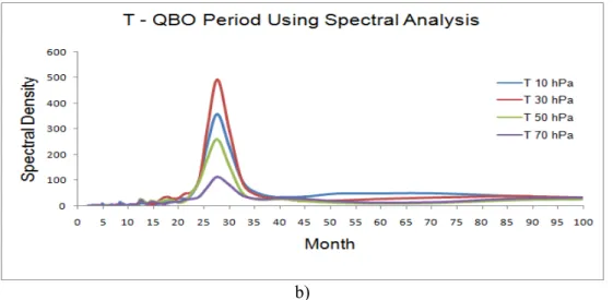
Based on spectral analysis, the oscillation of zonal wind shows a period of ~27.7 months (Figure 8a) at

~30 hPa above the surface. This result is marginally shorter than ~28.4 and ~28.2 months as measured by Baldwin et al (2001; observation) and Pascoe et al (2005; ERA-40) respectively. The similar period of oscillation is also occurred in temperature (Figure 8b).

Using cross-correlation method between zonal wind at 10 hPa and 30 hPa (Figure 9a) and at 10 hPa and 50 hPa (Figure 9b) above the surface, it can be calculated that QBO descends downward at rate of

~1.06 km/month. The result agrees with the propagation rate of ~1 km/month measured by Holton (2004).

a)

(11)

b)

Figure 8. Spectral Analysis method to determine the period of QBO. a) Periodicity value of QBO in zonal wind, b) Periodicity value of QBO in temperature.

Figure 9. Cross-correlation of zonal wind anomaly. a) Cross-correlation between zonal wind anomaly at 10 hPa and 30 hPa, b) Cross-correlation between zonal wind anomaly at 10 hPa and 50 hPa.

(12)

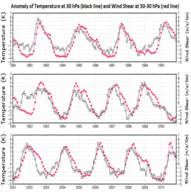
3.2.Relationship of Temperature and Wind Shear

Relationship of QBO-dU/dz (wind shear anomaly) and QBO-T (temperature anomaly) satisfies the thermal wind equation due to very small contribution of the mean meridional and vertical motion (Holton 2004). Anomaly of westerly wind shear associates with anomaly of warm temperature in the equator, and anomaly of easterly wind shear associates with anomaly of cold temperature (Pascoe et al 2005). Figure 10 shows the relationship between zonal mean of temperature anomaly at 30 hPa and zonal mean of wind shear anomaly at 50 – 30 hPa above the surface. Anomaly of temperature in QBO is consistent at ±4 K at 30 hPa (Baldwin et al 2001).

QBO is symmetry to the equator and the contribution of mean vertical and meridional motion is very small to the oscillation, so the relationship of wind shear and temperature in QBO satisfies the thermal wind equation. The equation can be formulated as follows :

(6)

In the equator, T 0 y

∂ =

∂ ^{due to} y=0. By using L’Hopital rule, the thermal wind equation in the equator can be formulated as follows :

(7)

Where uis zonal wind, T is temperature, z is log-pressure height, y is latitude, R is gas costant of dry air, H ≈7 km, and β is variation of Coriolis parameter in latitude (Andrews et al 1987).

The equation explains the meaning of Figure 10. Second derivative of temperature has an apposite sign with temperature in the equator, so wind shear and positive anomaly of temperature (warm) are in a same phase during the westerly phase of QBO. During the easterly phase of QBO, wind shear is in a same phase with negative anomaly of temperature (cold).

An exception is occurred in 1991, where temperature is suddenly increased (Figure 10 and 12). This event is caused by the eruption of Mt. Pinatubo (Philippine) on 14^th – 15^th of June 1991. The eruption created a giant cloud of aerosol in the stratosphere surrounding the earth during 2 weeks and spreading to the tropical region around 30⁰ N – 20⁰ S (McCormick and Veiga 1992). Sulphate aerosol of the eruption heated the stratosphere by absorbing the infrared radiation from the earth (Robock 2000). By absorbing the radiation, temperature in the stratosphere is significantly increased.

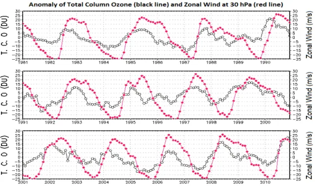
3.3.Association of QBO and Total Column Ozone (TCO) in the Stratosphere

Concentration of ozone in the stratosphere is resulted by a combination of transport and photochemistry process at ~30 – 20 hPa above the surface (Brasseur et al 1999). Figure 11 shows that there is a defference of ozone concentration in the westerly and easterly phase of QBO, where ozone concentration is relatively increased during the westerly phase of QBO, but decreased during the opposite phase. It indicates the transport process of zonal wind oscillation in QBO to the fluctuation of ozone in the lower-stratosphere.

u R T

y z H y

β ^∂ = − ^∂

∂ ∂

2 2

u R T

z H

β

y

∂ ∂

∂ = − ∂

(13)

Figure 10. Relationship of temperature anomaly (T) at 30 hPa and wind shear anomaly (dU/dz) at 50- 30 hPa above the surface.

Ozone depletion is not only related to the depletion of ozone substances, but also related to temperature in the stratosphere. Negative anomaly of temperature in QBO (Figure 12) shows that lower temperature in the easterly phase of QBO is associated with the depletion rate of ozone causing the ozone depletion. In the other side, negative anomaly of TCO is generally associated with negative anomaly of temperature in QBO, because ozone absorbs the sun radiation and infrared radiation. The lower concentration of ozone in the stratosphere causes a lower absorbtion of radiation, so temperature is decreased in the lower-stratosphere. During the westerly phase of QBO, anomaly of temperature will be increased as long as TCO is increased.

(14)

Figure 11. Relationship of Total Column Ozone anomaly (TCO) and zonal wind anomaly (U) in QBO at 30 hPa above the surface.

Figure 12. Relationship of Total Column Ozone anomaly (TCO) and temperature anomaly (T) in QBO at 30 hPa above the surface.

(15)

4.Conclusion

The zonally symmetric easterly and westerly phase of QBO regimes alternate with period of ~27.7 months and descend downward at rate of ~1 km/month. Based on Equivalent QBO Amplitude (EQA) method, the maximum amplitudes of QBO in zonal mean zonal wind (u), temperature (T), wind shear (du/dz), and quadratic vertical shear (d²u/dz²) are ~28.3 m/s, ~3.4 K, ~4.8 m/s/km, and ~1.0 m/s/km² respectively which are generally occurred at ~30 – 20 hPa above the surface of the equatorial region.

The amplitudes are increased in the equator, but decreased exponentially with a Gaussian distribution in latitude.

QBO is not only to discuss about zonal wind oscillation, but also to discuss about the physical and chemical process in the lower-stratosphere. Relationship of wind shear and temperature satisfies the thermal wind equation due to very small contribution of the mean meridional and vertical motion.

Moreover, concentration of Total Column Ozone (TCO) is significantly influenced by QBO. During the westerly phase of QBO, the TCO is relatively increased in the lower-stratosphere, but decreased during the easterly phase of QBO.

5.References

[1] Andrews G A, Holton J R and Leovy C B 1987 Middle Atmosphere Dynamics (Orlando, FL:

Academic Press)

[2] Angell J K and Korshover J 1964 Quasi-biennial Variations in Temperature, Total Ozone, and Tropopause Height J. Atmos. Sci. 21 479-429

[3] Baldwin M P et al 2001 The Quasi-biennial Oscillation Rev. Geophys. 39 179-229

[4] Box E P and Jenkins G M 1976 Time Series Analysis: Forecasting and Control (Michigan:

Michigan University)

[5] Brasseur G P, Orlando J J and Tyndall G S 1999 Atmospheric Chemistry and Global Change (New York: Oxford University Press)

[6] Dee D P et al 2011 The ERA-Interim Reanalysis: Configuration and Performance of the Data Assimilation System Q. J. R. Meteorol. Soc. 137 553-597

[7] Ebdon R A 1960 Notes on the Wind Flow at 50 mb in Tropical and Subtropical Regions in January 1957 and in 1958 Q. J. R. Meteorol. Soc. 86 540-542

[8] Gray L J et al 2001b A Data Study of the Influence of the Equatorial Upper Stratosphere on Northern-Hemisphere Stratospheric Sudden Warnings Q. J. R. Meteorol. Soc. 127 1985- 2003

[9] Holton J R and Lindzen R S 1972 An Updated Theory for the Quasi-biennial Oscillation of the Tropical Stratosphere J. Atmos. Sci. 29 1076-1080

[10] Holton J R 2004 Introduction to Dynamics Meteorology (Burlington: Elsevier)

[11] McCormick M P and Veiga R E 1992 SAGE II Measurements of Early Pinatubo Aerosols Geophys. Res. Lett. 19 155-158

[12] Naujokat B 1986 An Updated of the Observed Quasi-biennial Oscillation of the Stratospheric Winds Over the Tropics J. Atmos. Sci. 43 1873-1877

[13] Pascoe C L et al 2005 The Quasi-biennial Oscillation: Analysis Using ERA-40 Data J.

Geophys. Res. 110 D08105 doi:10.1029/2004JD004941

[14] Randel W J et al 2004 The SPARC Intercomparison of Middle Atmosphere Climatologies, J.

Climate. 17 986-1003

[15] Reed R J, Campbell W J, Rasmussen L A and Rogers R G 1961 Evidence of a Downward Propagating Annual Wind Reversal in the Equatorial Stratosphere J. Geophyis. Res. 66 813- 818

[16] Robock A 2000 Volcanic Eruptions and Climate Rev. Geophys. 38 191-219