Partitioning of Ozone Loss Pathways in the Ozone Quasi-biennial Oscillation Simulated by a Chemistry-Climate Model

(1)

©The Author(s) 2020. This is an open access article published by the Meteorological Society of Japan under a Creative Commons Attribution 4.0 International (CC BY 4.0) license (https://creativecommons.org/licenses/by/4.0).

Partitioning of Ozone Loss Pathways in the Ozone Quasi-biennial Oscillation Simulated by a Chemistry-Climate Model

Kiyotaka SHIBATA

Kochi University of Technology, Kochi, Japan Meteorological Research Institute, Tsukuba, Japan

and Ralph LEHMANN

Alfred Wegener Institute, Helmholtz Centre for Polar and Marine Research, Germany (Manuscript received 9 October 2019, in final form 28 February 2020)

Abstract

Ozone loss pathways and their rates in the ozone quasi-biennial oscillation (QBO), which is simulated by a chemistry-climate model developed by the Meteorological Research Institute of Japan, are evaluated using an objective pathway analysis program (PAP). The analyzed chemical system contains catalytic cycles caused by NOx, HO_x, ClO_x, O_x, and BrO_x. PAP quantified the rates of all significant catalytic ozone loss cycles, and evaluated the partitioning among these cycles. The QBO amplitude of the sum of all cycles amounts to about 4 and 14 % of the annual mean of the total ozone loss rate at 10 and 20 hPa, respectively. The contribution of catalytic cycles to the QBO of the ozone loss rate is found to be as follows: NOx cycles contribute the largest fraction (50 – 85 %) of the QBO amplitude of the total ozone loss rate; HO_x cycles are the second-largest (20 – 30 %) below 30 hPa and the third-largest (about 10 %) above 20 hPa; Ox cycles rank third (5 – 20 %) below 30 hPa and second (about 20 %) above 20 hPa; ClO_x cycles rank fourth (5 – 10 %); and BrO_x cycles are almost negligible. The relative contribution of the NOx and Ox cycles to the QBO amplitude of ozone loss differs by up to 10 % and 20 %, respectively, from their contribution to the annual mean ozone loss rate. The ozone QBO at 20 hPa is mainly driven by ozone transport, which then alters the ozone loss rate. In contrast, the ozone QBO at 10 hPa is driven chemically by NO_x and the temperature dependence of [O]/[O₃], which results from the temperature dependence of the reaction O + O2 + M → O3 + M. In addition, the ozone QBO at 10 hPa is influenced by the overhead ozone column, which affects [O]/[O₃] (through ozone photolysis) and the ozone production rate (through oxygen photolysis).

Keywords quasi-biennial oscillation; ozone; chemistry-climate model; pathway analysis program; catalytic cycles Citation Shibata, K., and R. Lehmann, 2020: Partitioning of ozone loss pathways in the ozone quasi-biennial oscillation simulated by a chemistry-climate model. J. Meteor. Soc. Japan, 98, 615–636, doi:10.2151/jmsj.2020-032.

Corresponding author: Kiyotaka Shibata, School of Envi- ronmental Science and Engineering Kochi University of Technology, 185 Miyanokuchi, Tosayamada, Kami, Kochi 782-8502, Japan

E-mail: shibata.kiyotaka@kochi-tech.ac.jp J-stage Advance Published Date: 2 April 2020

(2)

1. Introduction

The quasi-biennial oscillation (QBO) in zonal wind and temperature is one of the largest variations in the equatorial stratosphere, and its effects can reach the extratropics as far as the North Pole (e.g., Baldwin et al. 2001). Together with the QBO in dynamical quantities, trace gases like ozone show similar oscilla- tions in the equatorial stratosphere due to the transport and/or chemistry associated with the QBO, and the corresponding ozone oscillation is thereby called the ozone QBO. Detailed vertical and temporal structures of the QBO in O3 and NO2 were revealed through Stratospheric Aerosol and Gas Experiment (SAGE) II data by Zawodny and McCormick (1991), Hasebe (1994), and Chipperfield et al. (1994) and through Global Ozone Monitoring by Occultation of Stars (GOMOS) data by Hauchecorne et al. (2010) and Liu et al. (2011). By analyzing the Optical Spectrograph and Infrared Imager System data, Park et al. (2017) have also showed the detailed structures of the QBO in O3, NOx, N2O, and HNO3. Unlike the zonal wind, temperature, and NO2, these studies demonstrated that the ozone QBO has a distinctly sharp phase change (transition) at around 28 km, where the transition occurs between dynamical control below and photochemical control above. The ozone and temperature signals are in phase below the transition altitude, while they are out of phase above it.

The ozone QBO in the dynamically controlled region is interpreted as being driven by transport due to vertical motion, which is a part of the secondary circulation of the QBO (Plumb and Bell 1982). On the other hand, the cause of the ozone QBO in the photochemically controlled region has not yet been fully determined. The sharp phase change in the ozone QBO has been investigated with numerical models.

Ling and London (1986), using a one-dimensional model, attributed the ozone QBO in the photochemically controlled region as the effect of temperature on the rate constants for reactions of ozone destruction.

On the other hand, Chipperfield et al. (1994) asserted that Ling and London (1986) have disregarded the feedback of the NO2 variations on the ozone by using a fixed NO2 profile, and he further demonstrated, using a two-dimensional model, that the ozone QBO above the transition altitude is due primarily to the NO – NO2 catalytic cycles of ozone destruction. Tian et al. (2006), using of a fully coupled chemistry- climate model (CCM) and a photochemical box model, confirmed that NOx is the main chemical driver of the ozone QBO above the transition altitude.

However, using a three-dimensional chemistry transport model without QBO-induced variations in odd nitrogen (NOy) transport, Butchart et al. (2003) reproduced the ozone QBO with a phase reversal (relative to the phase of the QBO of the horizontal wind) near 10 hPa and an amplitude consistent with observations.

The intermediate importance of NOx was detected by Fleming et al. (2002), who found that the QBO in odd nitrogen radicals plays a significant but not dominant role in determining the ozone QBO.

There exist many catalytic cycles of ozone destruction, and the dominant ones vary from one situation to another, depending on conditions such as temperature, solar zenith angle, altitude, and concentrations of ambient trace gases including ozone and aerosols.

Moreover, the analysis of catalytic cycles is primarily based on a predefined set of cycles, which is not nec- essarily the same in different studies (e.g., Wennberg et al. 1994; Jucks et al. 1996; Nevison et al. 1999).

Quantifying the contribution of each catalytic ozone destruction cycles is not straightforwardly performed, as different cycles may share some reactions, which makes the calculation of rates of cycles difficult. A quantitative evaluation of stratospheric ozone chemistry without the explicit specification of full catalytic cycles was made, e.g., by Osterman et al. (1997) and Meul et al. (2014). They evaluated the rate-limiting reactions, but did not aim at the ozone QBO. Oster- man et al. (1997) calculated the daily mean Ox production and loss rates by reactions involving different families of chemical species (NOx, HOx, ClOx, Ox, and BrOx) with a photochemical model, based on balloon observed data in the stratosphere at 34.5°N, 104.2°W in September 1993. Meul et al. (2014) quantified the ozone production and loss cycles in the tropical stratosphere under the current climate and for a projected climate at the end of the twenty-first century by per- forming an off-line evaluation of chemical reactions, in which 6-hourly CCM output for the temperature and a set of chemical constituents were used.

In this study, we use the pathway analysis program (PAP), developed by Lehmann (2002, 2004), to quantify the partitioning of catalytic ozone destruction cycles in the equatorial stratosphere. This program can objectively determine and evaluate (= assign a rate to) all significant pathways in chemical reaction systems.

So far, PAP has been utilized for various analyses such as:• Stratospheric and mesospheric ozone (Grenfell et al.

2006)

• Chlorine chemistry in the Antarctic lower stratosphere (Müller et al. 2018)

(3)

• Mesospheric nitric acid enhancements and ionic reactions affecting middle atmospheric HOx and NOy

during solar proton events (Verronen et al. 2011;

Verronen and Lehmann 2013)

• CO2 and ozone in the Martian atmosphere (Stock et al. 2012a, b; Stock et al. 2017)

• Photochemical reactions in super-Earth atmospheres (Grenfell et al. 2013)

This study aims to quantify the partitioning of ozone loss pathways caused by the following: nitrogen oxides (NOx = NO + NO2 + NO3), odd hydrogen (HOx

= H + OH + HO2), reactive chlorine (ClOx = Cl + ClO + 2 × Cl2O2), odd oxygen (Ox = O3 + O(³P) + O(¹D)), and reactive bromine (BrOx = Br + BrO) cycles in the ozone QBO simulated by the CCM of the Meteorolog- ical Research Institute (MRI) of Japan (MRI-CCM).

The dynamical features of the QBO simulated by MRI-CCM were investigated in detail by comparing them with those of the observed QBO (e.g., Shibata and Deushi 2008b; Naoe and Shibata 2010). The rest of this paper is arranged as follows. Section 2 describes the model, simulation conditions, and the chemical pathway analysis done by PAP. Section 3 presents the simulated QBO in dynamics and chemistry. Section 4 describes the partitioning of ozone loss cycles in the QBO as well as that in the annual mean.

The mechanism of the generation of the ozone QBO is investigated in more detail in Section 5, and lastly, conclusions are presented in Section 6.

2. Method

2.1 Chemistry-climate model

The MRI-CCM used in this study is nearly identical to the one used in previous studies (Shibata and Deushi 2008a, 2012), except for its increased number of vertical layers (81 instead of 68) to improve the vertical resolution in the upper stratosphere and mesosphere (above 10 hPa). The 81- and 68-layer CCMs are indicated as L81 and L68, respectively. Details of the previous MRI-CCM are described in Shibata and Deushi (2008a), that is why only a brief description of its dynamics and chemistry is provided here. The dynamics module of MRI-CCM is a spectral global model with triangular truncation, a maximum total wavenumber 42 (T42, about 2.8° by 2.8° in longitude and latitude grid space), and 81 layers in the eta-co- ordinate with a lid at 0.01 hPa (about 80 km). We call this version T42L81, which generates the QBO internally, similar to the previous T42L68, as will be shown later. The vertical spacing is about 500 m in the stratosphere between 100 hPa and 10 hPa, continuously increasing downward to the level of about 200 hPa

and upward to the model lid. The above-mentioned improvement of the vertical resolution above 10 hPa resulted in a more gradual layer broadening with a layer thickness of 1 ~ 2 km in the upper stratosphere and lower mesosphere. Non-orographic gravity-wave forcing by Hines (1997) is incorporated with an enhanced source strength of a Gaussian function equa- torward of 30°. Biharmonic (Δ²) horizontal diffusion is minimized only in the middle atmosphere compared to that in the troposphere to spontaneously reproduce the QBO in zonal wind while minimizing the changes in the troposphere (Shibata and Deushi 2005a, b).

In addition, vertical diffusion is not applied in the middle atmosphere to keep the sharp vertical shear in the QBO. The chemistry-transport module employs a hybrid semi-Lagrangian transport scheme compatible with the continuity equation to satisfy the mass conservation. The chemistry scheme treats 36 long- lived species including 7 families and 15 short-lived species with 80 gas-phase reactions, 35 photochemical reactions, and 9 heterogeneous reactions on polar stratospheric clouds and sulfate aerosols. The chemistry module of MRI-CCM was an update from the previous version (Shibata and Deushi 2008a, 2012) in the following points. The typographical error of the photolysis of CFC-12 (chlorofluorocarbon-12, CCl2F2) in JPL02 (Sander et al. 2002) was corrected to JPL06 (Sander et al. 2006). The Sun-Earth distance effect on photolysis was incorporated. The following three OH reactions were added: OH + OH → H2O + O, OH + OH + M → H2O2 + M, ClO + OH → HCl + O2, resulting in 83 gas-phase reactions. Nighttime chemistry was upgraded, so that it will be identical with the daytime chemistry except that photolysis rates and O(¹D) are set to zero at night. As a result, the simulated stratospheric ozone decreased, mainly due to the corrected CFC-12 photolysis.

The temporal change of ozone due to transport, in Section 5.2.a, is calculated as the difference between the ozone mixing ratios after and before a transport time step of the model. Similarly, the temporal change of ozone due to chemistry is evaluated as the difference between after and before chemistry calculation.

The overhead ozone column, found in Sections 5.2.b and 5.2.c, is defined at half-levels k-1/2, i.e., at the in- terface level between the adjacent upper layer k-1 and lower layer k. It is computed as a sum of the ozone concentration (multiplied by the layer thickness) from the top (k = 1) layer to the layer k-1, and hence it does not include the ozone in layer k. That is, the variations in the overhead column ozone at pressure level p do not include the variation of ozone in the layer at p.

(4)

2.2 Model simulation

The MRI-CCM of T42L81 version was integrated using an initial condition from L68 restart data on August 1 1970. It was under the CCMVal-2 B2 scenario (SPARC CCMVal 2010), i.e., REF-B2, which was made for simulations from 1960 to 2100, with a time-evolving forcing by greenhouse gases (GHGs), ozone depleting substances (ODSs), and sea surface temperature (SST) and with fixed solar minimum and background aerosol conditions in the stratosphere.

The integration was performed until November 2020, referred to as a standard run (ST run). Moreover, to collect the detailed chemistry data for PAP, i.e., rates of all the chemical reactions in the system and concentrations of all the species averaged over a time interval of interest, MRI-CCM of L81 was again run for a certain period, using the restart data at the end of relevant months of the ST run. One-day (24 hours) integrations were conducted every three months, i.e., for the first days of January, April, July, and October from January 1972 to April 1990, assuming that the sampling interval of three months is short enough to reproduce the overall features of the QBO (having a period of about two years) generated in the ST run.

The one-day integrations are called as pathway analysis run (PA run). As will be demonstrated later, the three-monthly 1-day mean data capture the general QBO characteristics in the ST run in spite of lacking certain temporal fine structures.

2.3 Pathway analysis program

The details of PAP are only briefly described here, as these are fully discussed by Lehmann (2002, 2004).

This is an algorithm that objectively determines all the significant pathways (reaction sequences) in an arbitrary chemical system. It may be summarized as follows. The algorithm starts from individual reactions. The chemical species in the system, one after the other, are treated as so-called “branching-points”.

For every branching-point species, each pathway pro- ducing it is connected with each pathway consuming it. If a newly formed pathway contains sub-pathways, e.g., null cycles, it is split into these simpler pathways.

Based on known reaction rates (usually from a chemical model run), the so-called “branching probabilities”

are calculated and used to determine a rate for each pathway. In order to avoid a too large number of pathways (“combinational explosion”), pathways with a rate smaller than a prescribed threshold are deleted during the construction process.

One advantage of PAP when used in ozone chemistry is its accurate and objective evaluation of the rel-

evant catalytic cycles of ozone loss by excluding null cycles. For example, one of the ozone loss reactions evaluated by Bruhwiler and Hamilton (1999) is OH + O3 → HO2 + O2. However, this reaction is also includ- ed in the following zero cycles, OH + O3 → HO2 + O2, HO2 + NO → OH + NO2, NO2 + hν → NO + O, and O + O2 + M → O3 + M, so that a significant fraction of the rate of this reaction does not lead to ozone loss.

As stated before, PAP requires a list of all the chemical reactions in the system, concentrations of all the species averaged over a time interval of interest, and rates of all reactions integrated over the same time interval. To prepare the full data for PAP, we set 32 equally spaced grid points at 1.4°N, nearest to the equator in T42 quadratic Gaussian latitudes, with the longitudinal interval being 11.25 degrees, and stored the rate constants and concentrations of chemical species at these grids before and after each chemistry time step of the model. Then we averaged the reaction rates and concentrations of chemical species on all the grid points at 1.4°N and all the time steps over the whole integration period, i.e., 24 hours. In principle, PAP should be applied for immediate chemical reactions, i.e., for one time-step of the integration of the differ- ential equations describing the chemical reactions, but it can also be applied for temporally averaged data (e.g., Grenfell et al. 2006).

3. Results of the simulation of the QBO 3.1 QBO of zonal wind and temperature

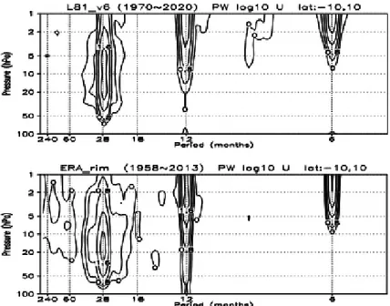
Figure 1 shows the power spectrum of the simulated and the observed zonal-mean zonal wind, latitudinally averaged within 10 degrees of the equator from 100 to 1 hPa. The simulated wind is taken from the ST run, in which the monthly mean data span 50 years from 1970 to 2020, while the observed wind is from the merged reanalysis data of ERA-40 (Uppala et al 2005) and ERA-Interim (Dee et al. 2011), spanning about 55 years from 1958 to 2013. There are three major modes of variability: semi-annual oscillation (SAO), annual cycle, and the QBO. The simulated QBO wind spectrum is quite similar to the observed one, with the center period being about 27 months in the simulation and 28 months in the observation, as in the previous version of the L68 MRI-CCM in the REF-B2 runs (Shibata and Deushi 2012). Although the simulated power spectrum of the QBO is similar to the observation, the observed QBO exhibits a more broadly spread spectrum, particularly in the far wing of longer periods. This is due in parts to the facts that the simulation includes neither the 11-year solar cycle nor volcanic aerosols from the three huge eruptions of

(5)

Agung, El Chichón, and Mount Pinatubo.

Figure 2 presents the anomalies of the observed (ERA-40) and the simulated zonal-mean zonal wind and temperature (averaged between 10°S and 10°N) from 70 to 5 hPa. It spanned for about 18 years from 1972 to 1990, together with the zonal-mean zonal wind anomalies at 30 hPa, in which anomalies are calculated by subtracting the mean annual cycle (averaged over all 18 years), in order to diminish the SAO, which is almost synchronized with the seasonal cycle.

It should be noted that the QBO phase is different in the observation and the simulation, because the simulated QBO is spontaneously generated with an average period of about one month shorter than the observation (Fig. 1). The simulated wind evidently reproduced the overall features of the observed QBO such as the faster downward propagation of westerly shear (defined as positive wind shear du/dz > 0) than easterly shear (du/dz < 0) as manifested in the zonal wind time series at 30 hPa (Figs. 2b, d). The temperature anomaly, the phase of which is approximately ad- vanced about one quarter cycle from that of the zonal wind anomaly, becomes positive (negative) during the westerly (easterly) shear due to the downdraft (updraft) associated with the meridional secondary circulation of the QBO (e.g., Plumb and Bell 1982). The temperature anomaly thereby provides useful information

as to the vertical transport of long-lived chemical species.

Before analyzing the PA run, we examined the effect of the different temporal averaging (monthly mean in the ST run and 1-day mean every three months in the PA run) on the QBO features in the zonal wind. Figure 3 shows the zonal wind anomalies obtained from the ST and PA runs at 1.4°N from 70 to 5 hPa between 1972 and 1990, together with zonal wind anomalies at 30 hPa, in which the anomalies of the PA run were calculated by subtracting an average value (over 18 years) for each calendar day present in the simulation. The 1-day mean data of the PA run certainly captures the QBO features of the stronger westerly shear as well as structures of strengths, dura- tions, and periods, whereas fine temporal and vertical structures are unavoidably lost as stated before. Sim- ilarly, we examined the effect of the latitudinal width of the analyzed model data. It was confirmed that the QBO at one latitude at 1.4°N (Fig. 3a) resembles that of a latitudinal average within 10 degrees of the equator (Fig. 2c). Meanwhile the former exhibits a slightly larger amplitude than the latter as expected, as from the QBO amplitude of the zonal wind maximizes over the equator (e.g., Randel et al. 1999; Pascoe et al.

2005). These comparisons indicate that the 1-day zonal-mean data at three-month intervals at 1.4°N can Fig. 1. Power spectrum of zonal-mean zonal wind from 100 to 1 hPa averaged between 10°S and 10°N (upper) in

the ST run from 1970 to 2020 and (lower) in the merged data of ERA-40 and ERA-Interim from 1958 to 2013.

Values are displayed in logarithmic scale of base 10, and units are m² s⁻². Contour interval is 0.4.

(6)

Fig. 2. Time-pressure cross sections of zonal wind anomalies [m s⁻¹] averaged between 10°S and 10°N shown from 70 hPa to 5 hPa for 1972 – 1990 (a) in ERA-40, (c) in the ST run, and (e) temperature anomalies [K] in the ST run.

Contour interval is 7 m s⁻¹ for wind and 2 K for temperature. In addition, zonal wind anomalies (axis range: from

−30 m s⁻¹ to 30 m s⁻¹) at 30 hPa of (b) ERA-40 and (d) the ST run.

Fig. 3. Time-pressure cross sections of zonal-mean zonal wind anomalies [m s⁻¹] at 1.4°N from 70 to 5 hPa for series of (a) monthly mean of the ST run and (c) 1-day mean at three-month intervals of the PA run, together with zonal wind anomalies (axis range: from −30 m s⁻¹ to 30 m s⁻¹) at 30 hPa of (b) the ST run and (d) the PA run. Con- tour interval in (a) and (c) is 7 m s⁻¹.

(7)

be utilized for the analysis of the QBO in the tropics.

3.2 QBO in the chemistry fields of O3 and NOx

Figure 4 presents the power spectrum of the simulated and the observed zonal mean ozone mixing ratio, which is latitudinally averaged within 10 degrees of the equator from 100 to 1 hPa. The observation is based on the combined satellite data of SAGE II and GOMOS for 1984 – 2011 (Kyrölä et al. 2013), in which missing data of about a quarter of the entire period are filled through interpolation on the isobaric surface. Meanwhile in the power spectrum of the simulated and the observed ozone, three major modes of variability, the SAO, annual cycle, and the QBO, are apparent, although the altitudinal distribution of their variability is significantly different from that of the zonal-mean wind. The difference in the spectral distribution of SAO, annual cycle, and the QBO between ozone and wind is the same as in Kumar et al. (2011).

Figure 5 displays the time-pressure cross sections of the absolute and relative anomalies of O3 and NOx, which is averaged between 10°S and 10°N of the ST run from 70 hPa to 5 hPa in the year 1972 – 1990.

Here, plots of NOx instead of NO2 (which is relevant for ozone loss, see Section 5.2.d) were presented, because NOx is less affected by diurnal variations.

NOx is almost entirely composed of NO and NO2

with a negligible contribution of NO3, in particular below about 5 hPa (Liu et al. 2011). Almost all NO

is converted to NO2 at night (e.g., Dessler 2000). On the other hand, at daytime, NO2 is determined by NOx

and the partitioning within NOx. However, since the variations of daily mean NO2 are found to be closely related to those of the daily mean NOx below about 10 hPa in the tropics, daily and monthly mean NOx can serve as a proxy of NO2 in this study, as in Park et al.

(2017).

The ST run reproduces significant decreasing trend of O3 in the upper stratosphere, which is about −1.3 % decade⁻¹ at 10 hPa (not shown), being in quantitative agreement with satellite observations (e.g., World Meteorological Organization 2003). The decreasing trend of the upper stratospheric O3 is attributed mainly to the increasing ClOx, which stems from the increasing surface emissions of ODSs in the CCMVal-2 B2 scenario.

The model reproduces the phase transition of the ozone QBO from dynamical to photochemical control at around 28 km (~ 18 hPa) in observations by SAGE II (e.g., Zawodny and McCormick 1991; Chipperfield et al. 1994) and GOMOS (Hauchecorne et al. 2010), which results in a dogleg-shape pattern with a vertex slightly above 20 hPa in the ozone anomaly. The simulated maximum amplitude at around 30 hPa (~ 24 km) of about 10 % in relative value (anomaly divided by its climatology), from +0.6 ppmv to −0.4 ppmv in abundance range, below the phase transition, is slightly smaller than observations. The amplitude of about Fig. 4. Power spectrum of zonal-mean ozone from 100 hPa to 1 hPa averaged between 10°S and 10°N (upper) in the

ST run from 1970 to 2020 and (lower) in the combined SAGE II-GOMOS ozone data from 1984 to 2011. Values are displayed in logarithmic scale of base 10, and units are (10⁻² ppmv)². Contour interval is 0.5.

(8)

4 % (~ 0.4 ppmv) at around 10 hPa (~ 31 km in the model) above the phase transition is quite identical to the observed values of about 5 % at 31 km (Zawodny and McCormick 1991; Chipperfield et al. 1994; Hau- checorne et al. 2010). While the O3 amplitude below 50 hPa is small in absolute values, it is much larger in relative values (not shown due to out of scale) than that at 30 hPa, being consistent with the GOMOS data (Hauchecorne et al. 2010).

The absolute NOx amplitude maximizes to about 0.7 pptv (~ 8 %) at 10 hPa. The relative amplitude is about 0.6 times of the observed values of about 13 % at 31 km (Zawodny and McCormick 1991; Chipper- field et al. 1994; Hauchecorne et al. 2010). In contrast to the ozone QBO, there is no phase reversal in the NOx QBO, to allow the NOx anomalies to propagate downward nearly continuously from the upper stratosphere like the temperature and wind anomalies. In addition, the absolute NOx amplitude is smaller below 20 hPa, i.e., in the dynamically controlled altitudes, than that above 20 hPa. This is also in contrast to O3, which shows substantial absolute amplitudes in both altitude regions.

4. Partitioning of ozone loss cycles in the QBO Shown in Tables 1 and 2 are the PAP results for the significant catalytic cycles, contributing more than 99 % to the total ozone production and those contributing individually more than 2 % to the total ozone destruction at 10 hPa and 20 hPa. It entails that the

production cycles lead to the net reaction 3O2 → 2O3, and all the destruction cycles result in 2O3 → 3O2. Chapman reactions are said to the responsible in the ozone production in the entire vertical range except for the lowermost level at 70 hPa, where production due to the smog cycles (e.g., Grenfell et al. 2006) contributes about 4.4 % (not shown). In contrast to the production, the ozone destruction is seen to be more complicated and involves many cycles. The type (i.e., chemical species involved), order, and rates of the destruction cycles differ depending mainly on the altitude, and thus the partitioning among them varies from one altitude to another as shown in Tables 1 and 2.

In what follows, we are going to consider families of species and, correspondingly, families of cycles, to simplify the presentation of the results, include also the contribution of minor pathways not shown in Tables 1 and 2, and elucidate the role of different families of chemical species. We will assign a cycle to a family of species (NOx, HOx, ClOx, BrOx, or Ox) if at least one reaction in the cycle contains a reactant from this family. However, we will assign a cycle to the Ox family only if it contains a reaction between two Ox species such as O + O3 → 2 O2. Otherwise, all ozone loss cycles would be assigned to the Ox family, as they contain the reactant O3. Moreover, the cycle (10-D2) is completely assigned to the NOx family (like (10-D1)), although it contains the reaction O(¹D) + N2

→ O + N2 of the Ox species O(¹D). This makes sense, Fig. 5. Time-pressure cross sections of (left) O3 and (right) NOx (upper) absolute and (lower) relative anomalies. All

data are detrended. Contour interval is 0.2 ppmv for absolute O3, 2 % for relative O3, 0.2 pptv for absolute NOx, and 3 % for relative NOx anomalies. Relative O3 anomalies are not shown below 50 hPa, because they are out of scale.

(9)

because the cycle (10-D2) is but identical to (10-D1), with the only difference in the O3 photolysis channel (O3 + hν → O(¹D) + O2, O(¹D) + N2 → O + N2 is equivalent to O3 + hν → O + O2). The same argument applies to both (20-D5) and (20-D1). It is possible that a cycle is assigned to more than one family, e.g., (10-D6) to NOx and ClOx. In this case, the rate of this cycle is divided by the number of these families, and the corresponding fraction of the rate is assigned to each family. For instance, half of the rate of cycle (10- D6) is assigned to NOx and the remaining half to ClOx. By this assignment, the net role of each family can be determined through the summation of the contribution

of each cycle at a specific time and altitude. For example, at 10 hPa, ozone destruction due to NOx-related cycles in Table 1 is about (357 + 76 + 30 + 0.5·25) ppbv day⁻¹ ≈ 476 ppbv day⁻¹. However, for the final analysis, also cycles with small rates, not contained in Tables 1 and 2, will be taken into account.

Here we denote the monthly mean ozone loss rate due to the catalytic cycles of family “i ” (NOx, ClOx, HOx, Ox, or BrOx) in month “l ” (January, April, July, or October) in year “k” of total “N ” years by δⁱ_kl. Then, the climatological (annual mean) ozone loss rate will be calculated as δⁱ_clim = (1/4N )å klδⁱ_kl for the cycles of family “i ”, which we also refer to simply as i-cycles Table 1. Daily and zonal mean ozone production and loss rates [ppbv day⁻¹]

of major catalytic cycles at 10 hPa, 1.4°N, January 1, 1980. Numbers in parentheses represent the absolute ozone change rate due to the corresponding production or destruction cycles and the same value relative to the total production or destruction.

1.4°N, January 1, 1980, daily-mean 10 hPa, Production

O2 + hv →O + O (627 ppb day⁻¹, 99.9 %)

2 × (O + O2 + M →O3 + M) (10-P1)

10 hPa, Destruction

O3 + hv →O + O2 (357 ppb day⁻¹, 54 %) O +NO2 → NO + O2

O3 +NO → NO2 + O2 (10-D1)

O3 + hv →O¹D + O2 (76 ppb day⁻¹, 12 %) O¹D +N2 →O +N2

O +NO2 → NO + O2

O3 +NO → NO2 + O2 (10-D2)

O3 + hv →O + O2 (54 ppb day⁻¹, 8 %)

O + O3 →O2 + O2 (10-D3)

O3 + hv →O¹D + O2 (30 ppb day⁻¹, 5 %) O¹D + O2 →O + O2

O +NO2 → NO + O2

O3 +NO → NO2 + O2 (10-D4)

O3 + hv →O + O2 (30 ppb day⁻¹, 5 %) ClO + O →Cl + O2

Cl + O3 →ClO + O2 (10-D5)

ClO +NO → NO2 + Cl

Cl + O3 →ClO + O2 (10-D6)

O3 + hv →O + O2 (16 ppb day⁻¹, 2 %) O + HO2 →OH + O2

OH + O3 →HO2 + O2 (10-D7)

O + O3 →O2 + O2 (10-D8)

(10)

or cycles, omitting sometimes “family”, henceforth.

Further, the monthly mean ozone loss rate is δ^sumkl

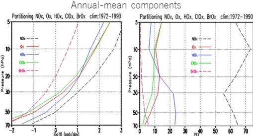
= å _iδⁱ_kl, and its climatological value is δ^sumclim = (1/4N ) å_klδ^sum_kl. Figure 6 shows the climatological vertical profile of the (a) absolute (δⁱ_clim) and (b) relative (δⁱ_clim/δ^sum_clim) contribution of each family of cycles from 70 hPa to 5 hPa. The ozone loss rate expressed as change of mixing ratio per day [ppbv day⁻¹], simply referred to as ozone loss rate henceforth, increases nonlinearly with altitude for all the cycles, with NOx

cycles accounting for the largest contribution in the entire vertical range. The contribution of other cycles differs, depending on altitude. For example, HOx

cycles are the second-largest contributor below 20 hPa, but fourth at 10 hPa. On the other hand, Ox and ClOx cycles, having much smaller rates than the HOx

cycles below 50 hPa, reach a similar magnitude as the HOx cycles at 20 hPa and yield the second- and

third-largest contribution above 10 hPa. Meanwhile, the contribution of BrOx cycles is very small: less than a few percentages above 30 hPa and, at most, several percentages in the lowermost stratosphere below 70 hPa.The absolute magnitude of each loss rate is about 10⁻² ~ 10⁻¹ ppbv day⁻¹ at 70 hPa and 10² ppbv day⁻¹ for ClOx, HOx, and Ox cycles and 10³ ppbv day⁻¹ for NOx cycles at 10 hPa, and thus the magnitude ranges are about 10⁴ from 70 hPa to 10 hPa. In contrast, BrOx

cycles have a similar loss rate as the Ox and ClOx

cycles in the lower stratosphere, but the increase of their rate with altitude is much lesser compared to that of the other cycles, which results in the magnitude range of about 10³. The relative magnitude, on the other hand, varies, depending on the altitude in certain ranges. NOx cycles contribute about 70 % at 10 hPa and about 60 % at other altitudes. HOx cycles con- Table 2. The same as Table 1 except for 20 hPa.

1.4°N, January 1, 1980, daily-mean 20 hPa, Production

O2 + hv → O + O (109 ppb day⁻¹, 99.7 %)

2 × (O + O2 + M →O3 + M) (20-P1)

20 hPa, Destruction

O3 +NO → NO2 + O2 (20-D1)

O3 + hv →O + O2 (10 ppb day⁻¹, 12 %)

O + O3 →O2 + O2 (20-D2)

HO2 + O3 →OH + 2O2 (7 ppb day⁻¹, 9 %)

OH + O3 →HO2 + O2 (20-D3)

O3 + hv →O + O2 (5 ppb day⁻¹, 6 %) ClO + O →Cl + O2

Cl + O3 →ClO + O2 (20-D4)

O +NO2 → NO + O2

O3 +NO → NO2 + O2 (20-D5)

O3 + hv →O + O2 (3 ppb day⁻¹, 3 %) O + HO2 →OH + O2

OH + O3 →HO2 + O2 (20-D6)

ClO +NO → NO2 + Cl

Cl + O3 →ClO + O2 (20-D7)

O3 + hv →O¹D + O2 (2 ppb day⁻¹, 2 %) O¹D + O2 →O + O2

O +NO2 → NO + O2

O3 +NO → NO2 + O2 (20-D8)

(11)

tribute slightly less than 10 % above 10 hPa and more than 20 % below 30 hPa, with an intermediate value of ~ 15 % at 20 hPa. Ox and ClOx cycles are very close to each other within a few percentages, and they increase gradually with altitude from a few percentages at 70 hPa to ~ 15 % at 5 hPa.

These vertical profiles of loss rates are qualitatively similar to those in other off-line evaluations of chemistry (e.g., Osterman et al. 1997; Meul et al. 2014).

But it is different in the lower stratosphere below 50 hPa, where HOx cycles are considered to be the second-largest contributor (about 25 %) and the largest one. These said cycles contribute about 50 % at a northern mid-latitude site of 34.5°N in September ac- cording to Osterman et al. (1997), or about 80 % in the tropics averaged from 25°S to 25°N as per Meul et al.

(2014). The discrepancy between the current results and those of Osterman et al. (1997) is at least partly caused by differences in season and location and in the abundances of chemical species: the simulated monthly zonal mean O3, H2O, and HO2 abundances at 35°N at 50 hPa reach the minimum values around October. Still, these values are slightly larger than the annual mean abundances over the equator. A reason for the larger contribution of HOx cycles in the study by Meul et al. (2014) is that they are splitting the zero cycle

OH + O3 → HO2 + O2, (R1)

HO2 + NO → OH + NO2, (R2)

NO2 + hν → NO + O, (R3)

O + O2 + M → O3 + M, (R4) into O3 production by reactions (R2)−(R4) and O3

loss by reaction (R1), which adds more contribution to the HOx cycles. Be that as it may, the partitioning of ozone loss in the lower stratosphere does not bring significant effects on the ozone mixing ratio, because the absolute values of the rates are very small. For instance, at 50 hPa, where the ozone mixing ratio is larger than 1 ppm, the loss rate is in the order of 1 ppb day⁻¹ ~ 1 ppm (3 yr)⁻¹ (Fig. 6).

Figure 7 shows the time series of the deviation of the rate of each family of cycles from its mean value relative to the total climatological value [(δⁱkl – δⁱclim)/

δ^sumclim]. It also provides the corresponding quantity for the total loss rate [(δ^sum_kl − δ^sum_clim)/δ^sum_clim] from 1972 to 1990 for each altitude (10, 20, and 30 hPa) in the PA run, in which all quantities are detrended. In the un-detrended raw fields, the ClOx cycles show a linearly increasing trend of about 5 % decade⁻¹ at 10 hPa and a slight upward trend with very small QBO variations at 20 hPa and 30 hPa (not shown). It should be noted that with the deviations of the catalytic cycles not perfectly but partly synchronized, the NOx

relative loss rate deviation sometimes exceeds the sum of relative loss rates deviations (e.g., in January of 1980 and July of 1982 at 20 hPa).

The QBO components of the other cycles can be straightforwardly identified at each altitude, although Fig. 6. Vertical profiles of the annual mean ozone loss rate by NOx, HOx, ClOx, Ox, and BrOx catalytic cycles shown

as (left) absolute values [ppbv day⁻¹] and (right) relative values [%] from 70 hPa to 5 hPa. Absolute values are displayed in logarithmic scale of base 10.

(12)

positive components and negative components do not have symmetric shapes, particularly at 20 hPa and 30 hPa. The positive components are like triangle waves, while the negative components are like square waves at 20 hPa and 30 hPa. The QBO phase descending across altitudes can be easily detected, while QBO characteristics such as amplitude and phase duration differ from one QBO cycle to another. In addition, the correlation of the QBO amplitudes across altitudes differs from one descending QBO to another. For example, the positive peak of the total loss rate in the middle of 1980 at 20 hPa is smaller than the previous peak in 1978 and the following peak in 1983, while it is the largest of the three at 10 hPa and 30 hPa. To quantitatively obtain QBO components of the ozone loss rate, a Lanczos bandpass filter with cut-off periods of 15 months and 60 months (i.e., 5 unit and 20 unit lengths of three-month intervals) is applied to the ozone loss rates in the PA run (Fig. 7) over the entire time series of δⁱ_kl from 1972 to 1990. After, the average QBO amplitude of each cycle (AδⁱQBO) is calculat-

ed as 2σ, where σ is the root mean square of the bandpass-filtered time series, by assuming a mono- chromatic wave. The same method is used for the sum of all cycles (δ^sum_QBO = å iδⁱ_QBO), so that the sum of the QBO amplitude of individual cycles is larger than the QBO amplitude of the sum of all cycles, å i AδⁱQBO >

Aδ^sumQBO, because all the cycles are not completely in phase.

Figure 8 exhibits the vertical profile of the QBO amplitude of each family of cycles, presented as (a) absolute (AδⁱQBO) and (b) relative (Aδⁱ_QBO /Aδ^sumQBO) values. Since å i AδⁱQBO > Aδ^sumQBO as stated above, the sum of the relative values exceeds 100 % by up to about 10 %. The absolute values of the QBO amplitudes are much smaller compared to those of the annual mean loss rates in Fig. 6. The QBO amplitude of the sum of all cycles amounts to about 4, 14, and 21 % of the annual mean of the total loss rate at 10, 20, and 30 hPa, respectively. The partitioning among the cycles, i.e., relative QBO amplitudes, more or less, resembles that of the annual mean for HOx, ClOx, and BrOx

Fig. 7. Time series of the deviation of the rate of each family of catalytic cycles from the corresponding mean rate relative to the total climatological ozone loss rate [(δⁱ_kl – δⁱ_clim)/δ^sum_clim] and the corresponding quantity for the total loss rate [(δ^sumkl − δ^sumclim)/δ^sumclim] at 10, 20, and 30 hPa from 1972 to 1990. All data are detrended.

(13)

cycles. However, NOx and Ox cycles are substantially different. The contribution of NOx cycles to the QBO of ozone loss is ~ 10 % smaller at 30 hPa and ~ 10 % larger at 10 hPa than the corresponding contribution to the annual mean ozone loss rate (shown in Fig. 6), whereas that of Ox cycles is several percentages larger at 50 – 10 hPa and 20 % larger at 5 hPa. Thus, the contribution of catalytic cycles to the QBO of the ozone loss rates can be summarized as follows: NOx cycles have the largest fraction, which amounts to 50 – 85 % of the QBO amplitude of the total ozone loss rate.

HOx cycles account for the second-largest contribution (20 – 30 %) below 30 hPa and the third-largest contribution (about 10 %) above 20 hPa. Meanwhile, Ox

cycles rank third (contributing 5 – 20 %) below 30 hPa and second (contributing about 20 %) above 20 hPa.

For ClOx cycles, they are in the fourth position with a nearly constant contribution of 5 – 10 %. Lastly, BrOx

cycles are almost negligible except below 50 hPa, contributing to around 3 – 5 %.

The ratio of the QBO amplitude of the two major catalytic cycles (Ox and NOx), Aδ^OxQBO /Aδ^NOxQBO, in the upper stratosphere is about 36 %/82 % ~ 0.44 at 5 hPa and about 20 %/85 % ~ 0.24 at 10 hPa. Tian et al.

(2006) made a similar estimation using photochemical box model initialized with CCM output every 10 days over a 20-year simulation. They found that at 35 km (corresponding to 7 hPa in MRI-CCM), the QBO amplitude of Ox loss due to NOx (reaction NO2 + O) is ~ 2.8 % of the total Ox loss and that due to Ox is

~ 0.7 %. Hence, the corresponding ratio of the QBO amplitudes is Aδ^OxQBO /Aδ^NOx_QBO ~ 0.7 %/2.8 % ~ 0.25,

which lies between the above-mentioned values of 0.24 (at 10 hPa) and 0.44 (at 5 hPa) in the present study.

5. Mechanism of the ozone QBO

To understand the regime change of the ozone QBO around 28 km, we investigated the dominant processes at two altitudes in more detail: 20 hPa (~ 26 km) in the dynamically controlled region and 10 hPa (~ 31 km) in the chemically controlled region. The ozone mixing ratio in the ascending branch of the Brewer-Dobson circulation, i.e., background ozone, is mainly determined by the combined action of vertical upward transport and chemical production and loss (resulting in chemical net ozone production in the lower stratosphere) during this ascent. Thereby, the ozone QBO, which is an anomaly component superimposed in the background ozone, is also governed by the combined action of vertical transport and chemistry.

5.1 Dynamically controlled region

At the dynamically controlled altitudes below 20 hPa, a consistent structure is maintained in the QBO between zonal wind, temperature, and chemical species through the secondary meridional circulation.

In the westerly shear, i.e., during a strengthening of westerly zonal wind, there is a QBO-induced downdraft (Plumb and Bell 1982), which counteracts the background upward motion of the Brewer-Dobson circulation (Randel et al. 1999, Fig. 14; Fleming et al.

2002, Fig. 1). This QBO-induced downdraft induces adiabatic warming with cancelling radiative cooling.

Fig. 8. Same as Fig. 6 except for the QBO amplitude.

(14)

Moreover, it has the effect that the vertical motion of air through the region of net ozone production (by O2

photolysis) is slower, providing more time for ozone production in ascending air parcels and, thus, more ozone in this air. As there is net NOx production (from N2O) in the lower stratosphere, arguments similar to those for O3 also apply to NOx. During easterly shear, the QBO generates an additional upward motion, changing the above argumentation to the opposite.

These features are clearly shown in the non-filtered time series of zonal wind, temperature, O3, NOx, and ozone loss rate anomalies at 20 hPa (Fig. 9) in the PA run. Temperature precedes zonal wind by about a quarter cycle and is in phase with ozone.

Shibata and Deushi (2005b, Fig. 5) reproduced the

phase relationships among wind, temperature, and ozone in three-dimensional model runs both with and without a feedback of ozone on temperature; this indicates that the feedback of ozone does not play a vital role on the phase relationship. Using the mechanistic one-dimensional model of Lin and London (1984), utilizing a simple linear damping term instead of a realistic chemical scheme, Hasebe (1994) concluded that the ozone solar heating feedback is key to reproduce this phase relation in the ozone QBO in the lower stratosphere. However, though not stated explicitly, the results of the study of Hasebe (1994, Figs. 6, 7) demonstrate that even the chemical effect alone can also reproduce a similar phase relation above 30 hPa, in agreement with a simulation with no feedback of Fig. 9. Time series of zonal-mean anomalies of (a) zonal wind [m s⁻¹], (b) temperature [K], (c) O3 [%], (d) NOx [%],

and (e) total ozone loss rate [%] at 20 hPa in the PA run.

(15)

ozone on temperature by Shibata and Deushi (2005b).

There is still another potential mechanism for this phase relation. Bruhwiler and Hamilton (1999) demonstrated ozone horizontal transport by eddies to play a key role, at least in the vicinity of 40 hPa, through a GCM experiment with a non-interactive chemistry and nudged QBO forcing.

As the QBO amplitude of the ozone production is very small (Fig. 10, bottom), the variation of the net chemistry tendency (= production minus loss) of ozone is nearly identical to that of the loss rate alone (Fig. 10, bottom), so that, for investigating the role of chemistry, it is sufficient to consider only ozone loss.

Figures 9 and 10 (bottom) show that the ozone loss rate (counted positive in the case of loss) is in phase with ozone; equivalently, the chemistry tendency is out of phase with ozone, similar to the results obtained at 30 hPa by Naoe et al. (2017). The phase relation among ozone, chemistry, transport, and net (addition of chemistry and transport) tendencies of the QBO components in the ST run is presented in Fig. 11. This phase relation demonstrates that the driving process of the ozone QBO at 20 hPa is not chemistry, but transport. The chemical ozone loss counteracts the ozone anomaly induced by transport and contributes to the phase shift of the ozone net tendency, which advances

ozone by a quarter cycle (Fig. 11).

The magnitude of the relative QBO amplitude of the ozone loss rate (≈ 20 %) (Figs. 9e, 7, middle panel) may be roughly explained by the relative amplitudes of ozone (≈ 5 %) and NOx (≈ 10 %) (Figs. 9c, d) and a contribution from the temperature variation of reaction rate constants (mainly KO+O2+M of the reaction O + O2 + M → O3 + M, affecting the ratio of the concentrations of atomic oxygen and ozone and KO+O3

of the reaction O + O3 → 2 O2 in the Ox cycles).

5.2 Chemically controlled region

In the photochemically controlled altitudes above about 10 hPa, a dynamical structure similar to that at 20 hPa is still maintained between the QBO of zonal wind and temperature, with temperature preceding zonal wind by a quarter cycle as displayed in the time series at 10 hPa in the PA run (Fig. 12). The phase of NOx lies between the phases of temperature and zonal wind. This slight advance of NOx relative to the zonal wind at 20 hPa and 10 hPa is very similar to the feature of the lag-correlation between NO2 and the zonal wind in SAGE II data (Hasebe 1994). The bandpass-filtered QBO time series in the ST run confirms that the phase relations between temperature and NOx

are identical to those at 20 hPa (not shown). However, Fig. 10. Three-month interval series of the QBO ozone loss rate (-L, black), production rate (P, red), net production

rate (P-L, green), and O3 (dashed blue) at (upper) 10 hPa and (lower) 20 hPa in the PA run from 1975 to 1984. The QBO components are bandpass-filtered (15 – 60 months) data. Units are ppbv day⁻¹ for loss rate and production rate and ppmv/30 for ozone.

(16)

ozone exhibits a different behavior. It is anti-correlated with temperature and zonal wind, so that the ozone maxima occur between temperature minima and zonal wind minima. Ozone is nearly out of phase with NOx. The QBO amplitude of ozone at 10 hPa is ≈ 4 %. In the next subsections, we are going to determine which factors contribute to this amplitude.

a. Ozone transport versus chemistry

The QBO amplitude of the temporal variation of ozone due to transport is ≈ 15 ppb day⁻¹ (Fig. 11d).

This is quite similar to the QBO amplitude of the ozone production rate as shown in Fig. 10 (upper panel). Consequently, both processes yield approximately equal contributions to the ozone variation.

The relative contribution [%] of the ozone production, yielding a minor contribution to the ozone QBO, is discussed in more detail in Section 5.2.b.

The net production rate advances from ozone by about a 1/8 cycle (Fig. 10, upper panel). Ozone transport, on the other hand, is nearly out of phase to ozone in the bandpass-filtered QBO (Fig. 11d). This out of phase relation between transport and ozone indicates that transport does not drive the ozone QBO.

Nevertheless, transport is but indispensable to make a phase advance of a quarter cycle for the net tendency against ozone. Accordingly, this phase relation among ozone, chemistry, and transport demonstrates that chemistry is a dominant driving force of the ozone QBO, although transport still plays a minor but significant role. This phase relation of chemistry to ozone at

10 hPa is in a sharp contrast to that in the dynamically controlled altitudes such as at 20 hPa (lower panel in Fig. 10), where chemistry (almost loss rate alone) and ozone are nearly out of phase as discussed in Section 5.1.

b. Chemistry: ozone production versus ozone loss Since the production of ozone is attributed solely to Chapman reactions, involving the photolysis of O2

(Table 1), an increase of the overhead ozone column immediately decreases the ozone production rate as solar ultraviolet irradiation is reduced, relevant for the photolysis rate coefficient JO2 (O2 + hν → O + O), reaching 10 hPa. Analogously, a decrease of the overhead ozone column increases the ozone production.

This would provide an explanation to the almost out of phase relation between the QBO components of the ozone production rate and the overhead column ozone (Fig. 13). The QBO amplitude of the O3 production rate is slightly less than 2 % (Fig. 13). This is consid- erably smaller than the QBO amplitude of the ozone loss frequency, which is discussed in more detail in Section 5.2.c.

c. Chemical ozone loss: NO_x variations versus temperature variations

As was shown in Section 4, at 10 hPa, the NOx

cycles contribute about 85 % of the QBO amplitude of the ozone loss rate (Fig. 8), which is consistent with the results obtained by Ling and London (1986), Chipperfield et al. (1994), and Tian et al. (2006). That Fig. 11. QBO component time series of zonal and monthly mean ozone and its tendencies in the ST run from 1975

to 1985. (a) Ozone [ppmv] (dashed curve) and net tendency [ppmv (100d)⁻¹] (solid curve) at 20 hPa, (b) chemical (long-dashed), transport (dotted with crosses), and net (quadrupled, solid) tendencies [ppmv (10d)⁻¹] at 20 hPa. (c) The same as in (a) except for 10 hPa. (d) The same as in (b) except for 10 hPa.

(17)

is why we are going to investigate the causes of variations of the rate of the NOx cycles in more detail in this subsection.

The rate-limiting reaction in the NOx cycles shown in Table 1 is O + NO2 → NO + O2 (with the rate constant KO+NO2). The rate of this reaction is

KO+NO2·[O]·[NO2]

= KO+NO2·([O]/[O3])·([NO2]/[NOx])·[NOx]·[O3], (1) where [ ] denotes the concentration of a chemical species. Consequently, the reaction rate may be rewritten as ΛO+NO2·[O3], where ΛO+NO2 is the corresponding ozone loss frequency (Dessler 2000):

Fig. 12. Time series of zonal mean anomalies of (a) zonal wind [m s⁻¹], (b) temperature [K], (c) O3 [%], (d) NOx [%], and (e) total ozone loss rate [%] at 10 hPa in the PA run.

Fig. 13. QBO component time series (at 10 hPa) of the daily mean ozone production rate [%]

(solid curve with open circles) in the PA run and the monthly mean overhead column ozone [%]

(dashed curve with plus signs) in the ST run.

Both data are zonally averaged values.

(18)

ΛO+NO2 = KO+NO2·([O]/[O3])·([NO2]/[NOx])·[NOx].

(2) As the NOx cycles destroy two ozone molecules, the corresponding ozone loss rate is 2·ΛO+NO2·[O3]. The time series of anomalies of ΛO+NO2 is shown in Fig.

14e. It has an amplitude of ≈ 10 %.

As shown in Eqs. (1) and (2), the ozone loss frequency is dependent on four factors: KO+NO2, [O]/[O3], [NO2]/[NOx], and [NOx]. We investigate how these quantities are modulated by the QBO of temperature and [NOx]:

a) KO+NO2 depends slightly on temperature, being negatively correlated with it. Its QBO amplitude is about 1 % (Fig. 14a).

b) [O]/[O3] has a QBO amplitude of ≈ 5 %. It is determined by the equilibrium of the O production by ozone photolysis and the O loss by the reaction O + O2 + M → O3 + M. The ozone photolysis frequency mostly depends on the overhead ozone column, as it has a decreasing trend and a QBO amplitude of ≈ 2 % (Fig. 14d). Meanwhile, the rate constant KO+O2+M of the three-body reaction O + O2

+ M → O3 + M depends significantly on tempera- Fig. 14. Time series of low-pass filtered anomalies of (a) KO+NO2 [%] (red curve) and [NO2]/[NOx] [%] (black curve),

(b) [O]/[O3] [%] (red curve) and NOx [%] (black curve), (c) temperature [K] (red curve) and O3 [%] (black curve), (d) 1/KO+O2+M [%] (red curve) and 1/(over_head_O3) [%] (black curve), and (e) ΛO+NO2 [%], and (f) [NOx]/[NOy] [%]

at 10 hPa in the ST run. All data are zonally and monthly averaged values. The cut-off period is 10 months.

Partitioning of Ozone Loss Pathways in the Ozone Quasi-biennial Oscillation Simulated by a Chemistry-Climate Model

Partitioning of Ozone Loss Pathways in the Ozone Quasi-biennial Oscillation Simulated by a Chemistry-Climate Model

(a)

(b) (c) (d) (e)

(f)