Observing sea ice thickness variability in the Laptev Sea and the implications

(1)

Observing sea ice thickness variability in the Laptev Sea and the implications

for the Transpolar Drift system

Dissertation submitted by

Hans JAKOB Belter

in partial fulfilment of the requirements for the degree of

Doctor of Natural Sciences (Dr. rer. nat.)

to Faculty 1

Physics and Electrical Engineering University of Bremen

Colloquium: January 12, 2021

(2)

Polar and Marine Research, Bremerhaven]

1. Reviewer:

Prof. Dr. Christian Haas

[Alfred Wegener Institute, Helmholtz Centre for Polar and Marine Research, Bremerhaven]

[University of Bremen]

2. Reviewer:

Prof. Dr. Torsten Kanzow

[Alfred Wegener Institute, Helmholtz Centre for Polar and Marine Research, Bremerhaven]

[University of Bremen]

This dissertation was written at the Sea Ice Physics section of the Al- fred Wegener Institute, Helmholtz Centre for Polar and Marine Research, Bremerhaven.

(3)

Abstract

The Arctic sea ice cover is strongly connected to the global climate system and therefore not only subject to internal variability but also in a phase of significant change related to the ongoing increase in global mean surface temperatures. The most important parameters to monitor and describe sea ice are its areal extent, thickness, and motion. While reliable, long-term satellite measurements of sea ice concentration, which is used to derive the area covered by sea ice, exist since the late 1970s, sea ice thickness and motion data sets of comparable quality and length are currently not available.

The overarching goal of this dissertation is to contribute to the improvement of sea ice thickness observations and to understand and quantify the impact of ongoing sea ice thickness changes and variability in the most important regions of sea ice formation on the overall Arctic sea ice budget. To achieve that, the first study presented in this dissertation focuses on extending the knowledge about sea ice thickness variability in the Laptev Sea by developing a new method to derive sea ice thickness time series from moored sonars. It is shown that daily mean sea ice thickness time series can be inferred from basic, moored upward-looking Acoustic Doppler Current Profilers. This adaptive approach allows to revisit data sets from past mooring deployments in the Laptev Sea and exploit them to extend the available sea ice thickness records and close observational gaps in a region that, due to its limited accessibility, is vastly under-sampled.

These new data sets are the basis for the validation of multiple satellite sea ice thickness products, including the longest available one introduced by the European Space Agency, which provides Arctic-wide sea ice thickness since 2002. It is shown that in the first-year ice dominated Laptev Sea the investigated satellite products provide the most frequently occurring (modal) rather than the mean sea ice thickness. This important discovery allows for a better interpretation of the available satellite records, especially for the investigation of sea ice volume transports, and underlines their deficiencies in representing dynamically deformed sea ice.

Based on the knowledge gained in the Laptev Sea, the final study presented in this dissertation follows the Arctic sea ice life cycle from the regions of ice formation along the Transpolar Drift towards Fram Strait and analyses whether sea ice thickness anomalies induced in the source regions of Arctic sea ice propagate to the central Arctic Ocean and beyond. More specifically, it is investigated which particular processes are potentially responsible for the induced anomalies in the source regions and whether their signals persist until the end of the Transpolar Drift. In the absence of a single-source Arctic- wide, high temporal and spatial resolution sea ice thickness data product, this final part promotes the combination of different techniques and tools for the investigation of this complex Arctic climate parameter. At the center of the investigation is an extended long-term electromagnetic induction sounding-based sea ice thickness time series, which shows a general thinning and decreasing age of sea ice at the end of the Transpolar Drift between 2001 and 2020. Due to its length, this unique time series also permits to put ice thickness measurements conducted during the Multidisciplinary drifting Observatory for the Study of Arctic Climate (MOSAiC) expedition into the historical context. Lagrangian ice tracking and modelling of thermodynamic sea ice growth along the pathways of Arctic

(4)

The presented efforts are an important contribution to the better understanding of Arctic sea ice thickness variability and change and can be seen as starting points for more targeted analyses of the driving mechanisms behind them. In addition, the acqui- sition, validation, and extension of sea ice thickness observations provide the basis for more detailed sea ice modelling, which will improve not only the monitoring but also the prediction of Arctic sea ice thickness changes in the future.

(5)

Nomenclature

Abbreviations

AARI Arctic and Antarctic Research Institute ADCP Acoustic Doppler Current Profiler

AEM Airborne electromagnetic induction instrument

AOI Area of interest

ARTIST Arctic radiation and turbulence interaction study ASSIST Arctic Shipborne Sea Ice Standardization Tool

AW Atlantic Water

AWI Alfred Wegener Institute, Helmholtz Centre for Polar and Marine Research BMBF Bundesministerium f¨ur Bildung und Forschung

BT Bottom track

CCI-2 Climate Change Initiative Phase 2

CDR Climate data record

CERSAT Center for Satellite Exploitation and Research

CO MOSAiC Central Observatory

CRISTAL Copernicus Polar Ice and Snow Topography Altimeter

CS2 CryoSat-2

CS2SMOS Merged weekly CS2 and SMOS sea ice thickness data record

DN MOSAiC Distributed Network

DNR Combined CO and DN regions (wider area around the MOSAiC floe) ECMWF European Centre for Medium-Range Weather Forecasts

EASE Equal Area Scalable Earth EM Electromagnetic induction ENVISAT Environmental Satellite

ERA ECMWF Re-Analysis

ESA European Space Agency

FDD Freezing degree days

FYI First-year ice

(8)

IBCAO International Bathymetric Chart of the Arctic Ocean ICESat-2 Ice, Cloud, and land Elevation Satellite 2

IPCC Intergovernmental Panel for Climate Change IPS Ice Profiling Sonar

MOSAiC Multidisciplinary drifting Observatory for the Study of Arctic Climate

MYI Multi-year ice

NAOSIM North Atlantic Arctic Ocean Sea Ice Model NSIDC National Snow and Ice Data Center

OSISAF Ocean and Sea Ice Satellite Application Facility PDF Probability Density Function

QUARCCS Quantifying Rapid Climate Change in the Arctic:

regional feedbacks and large-scale impacts RFBR Russian Foundation for Basic Research RMSE Root Mean Square Error

RV Research vessel

SIC Sea ice concentration SIT Sea ice thickness

SMOS Soil Moisture and Ocean Salinity SSM/I Special Sensor Microwave/Imager STK Shipborne television complex

SYI Second-year ice

ULS Upward-Looking Sonar

VAL Sonar-derived satellite validation data

(9)

Symbols

β Sound speed correction factor

D Vertical spacing between ULS pressure and range sensor [m]

d Sea ice draft [m]

η Instrument depth [m]

F Ocean heat flux [W m⁻²]

f Thermodynamic ice growth/decay function g Local gravitational acceleration [m s⁻²]

∆H

∆t Ice growth rate [m s⁻¹] H_ice Sea ice thickness [m]

H_snow Snow thickness [m]

h_i Distance EM device to air-snow/ice interface [m]

h_w Distance EM device to ice-water interface [m]

i Number of ADCP beams IT D Ice thickness distribution

κ_ice Thermal conductivity of ice [2 W m⁻¹K⁻¹] κ_snow Thermal conductivity of snow [0.33 W m⁻¹K⁻¹] L Latent heat of fusion [3·10⁸J m⁻³]

p_uls Pressure at ULS [hPa]

p_atm Pressure at sea surface [hPa]

Φ Redistribution function φ ADCP instrument tilt [^◦] ρ Density of seawater [kg m⁻³]

r Range [m]

σ_d Uncertainty of hourly mean sea ice draft from ADCP [m]

σ_r_φ Uncertainty of tilt-corrected ADCP range [m]

σ_z Uncertainty of ADCP-derived instrument depth [m]

T₀ Temperature at the ice-water interface [−1.86^◦C]

T_surf Sea surface temperature [^◦C]

(10)

θ ULS instrument tilt [ ]

#»v Ice drift velocity

x Location

z Derived quasi-depth of ADCP [m]

(11)

1 Introduction

1.1 Arctic sea ice and its role in the Earth’s climate system

The Arctic is one of the key regions of interest in the Earth’s complex and variable climate system. Global changes in climate-relevant parameters, like the increase in global mean surface air temperature, are amplified in the Arctic (Chapman and Walsh, 1993). In the recent decades, the Arctic mean surface air temperature anomaly has been nearly two to three times higher than the global mean (Hansen et al., 2010; Screen and Simmonds, 2010; Pithan and Mauritsen, 2014), which continues to have vast implications for one of the Arctic’s key components – sea ice.

Sea ice forms when seawater freezes. Due to its low density compared to seawater, sea ice floats at the interface between ocean and atmosphere and, together with the above snow cover, forms an insulating layer for the exchange of heat, mass, and momentum between the two climate components (McPhee, 2017). Due to the reflective surfaces of sea ice and snow, sea ice is an important component of the surface energy budget. Therefore, changes in the composition of sea ice and its areal extent can have major implications for the exchange of energy at the ocean surface. One example is the ice-albedo feedback first discussed by Budyko (1969), which describes a positive feedback mechanism induced by changes in the fraction of solar radiation reflected by the ice-covered ocean surface, known as albedo. Simplified, a reduction of sea ice area exposes more of the comparably dark ocean surface to the atmosphere. The albedo of the surface reduces and more solar radiation is absorbed, which subsequently leads to more warming of the ocean surface layer. This induced warming leads to sea ice melt, further reduction of the area covered by sea ice and even more energy-uptake by the ocean (Hall, 2004).

With the upper part of the ice cover protruding above the water level (ice freeboard) and the lower part being submerged into the water (ice draft), sea ice is exposed to influences from, but also interacts with, the atmosphere above and the ocean below.

Sea ice impacts surface ocean properties and stratification through freshwater release during melt and brine rejection in the upper ocean layer during sea ice formation. The changes in upper ocean density resulting from sea ice formation and melt contribute to the thermohaline ocean circulation, which is an integral part of the global ocean circulation (Rahmstorf, 2003). These few processes are single examples of the much more complex effects and interactions sea ice has on and with the Arctic climate system and show why it is considered a valuable indicator for variability of the Arctic climate but also ongoing global climate change.

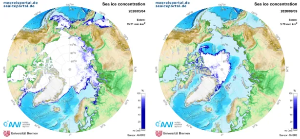
One of the most common parameters used to describe sea ice is its areal coverage.

Based on sea ice concentration data, regions covered by ice are described using sea ice area and extent. While sea ice area is a measure for the actual area covered by ice (km²), sea ice extent refers to gridded fields of data and whether single grid cells are considered ice-covered or not. Commonly, grid cells with sea ice concentrations of at least 15% are

(12)

Figure 1.1: AMSR-2 sea ice concentration data (Spreen et al., 2008) from the days of maximum extent on March 4, 2020 (left) and minimum extent on September 9, 2020 (right) obtained from www.seaiceportal.de (accessed October 2020).

considered ice-covered and the entire grid cell contributes to the total sea ice extent.

Therefore, the value of sea ice extent is usually higher than the area value.

Since the year 2000, Arctic sea ice covers between 14 and 16×10⁶km² at its maximum extent in winter (Comiso et al., 2017) including the whole central Arctic Ocean and most parts of the adjacent seas (example for March, 2020 in Fig. 1.1 (left)). During the summer melt season, the ice edge retreats to the central Arctic Ocean and sea ice covers only between 3.5 and 8×10⁶km² (Comiso et al., 2017) when it reaches its minimum extent in September (example for September, 2020 in Fig. 1.1 (right)). The region covered by sea ice during the extent minimum in summer marks the permanent ice zone. It consists of sea ice that has survived at least one melt season and is therefore considered multi-year ice (MYI). The seasonal ice zone is defined as the area of ocean between the permanent ice zone and the boundary of the sea ice extent maximum. It is partly covered by ice during the year and dominated by first-year ice (FYI, ice that has not survived a full melt season).

Solely observing sea ice extent only allows for a differentiation between ice covered and open water areas. Combining observations of sea ice extent, thickness, and motion are required to describe overall changes of the Arctic sea ice mass balance. The consideration of the temporal development of the most important sea ice parameters, extent and thickness, indicates a connection to observed trends in global surface air temperatures. The overall area covered by sea ice is reducing in all months (Cavalieri and Parkinson, 2012;

Comiso et al., 2017; Stroeve and Notz, 2018), while sea ice in general is thinning (Kwok, 2018). Due to the impact of sea ice on the surface energy and mass budgets, continuous decline in extent and thinning will increase the direct interaction between atmosphere and ocean with major implications for the entire Arctic ecosystem.

(13)

1 Introduction 1.1 Arctic sea ice

The predicted total summer sea ice loss is projected to change not only the Arctic, but also the global climate system severely (Stroeve et al., 2012; Overland and Wang, 2013; Overland et al., 2019). According to the Intergovernmental Panel for Climate Change (IPCC), these climatic changes will also have extensive socioeconomic impacts in the Arctic (Larsen et al., 2014). Besides new possibilities for economic diversification, shipping, forestry, and tourism, which are considered positive impacts, the loss in sea ice cover and permafrost may cause damage to all kinds of infrastructure used and built in the Arctic and impact the livelihoods of indigenous communities (Larsen et al., 2014).

In the context of global climate change, the discussions about observed trends in sea ice extent and thickness mostly refer to changes on an Arctic-wide scale. However, a more detailed analysis of the Arctic sea ice cover reveals that strong regional and seasonal variability exists (Haas, 2017). Therefore, observations of sea ice have to meet the expectation of the highest possible resolution on both temporal and spatial scales to monitor this variability. While satellite observations provide reliable, year-round, long- term sea ice extent and concentration records, sea ice thickness records of comparable length and quality are not available to this date. Satellite sea ice thickness records cover a much shorter period than sea ice extent and concentration records, are available only during the winter season, and have mostly been validated in regions dominated by MYI.

Considering the trend towards thinner and younger sea ice dominating the Arctic (Kwok, 2018), it is eminently important that satellite sea ice thickness data sets are continued, extended to the summer season, and validated for FYI-dominated regions.

One of these FYI-dominated regions is found in the eastern Arctic and especially in the Laptev Sea (Reimnitz et al., 1994). The Laptev Sea is considered one of the most important source regions of Arctic sea ice (Rigor et al., 2002; Hansen et al., 2013).

The prevailing offshore-directed winds transport newly formed ice away from the shelf seas, exposing vast areas of open water to the cold atmosphere, which leads to more ice formation in the shallow waters (Timokhov, 1994; Krumpen et al., 2013). This makes the Laptev Sea a region of major interest for the long-term development of Arctic sea ice.

The ice transported northward from the Siberian coast is incorporated into the Transpolar Drift system, which acts as a conveyor belt moving ice across the central Arctic Ocean towards the Fram Strait (Rigor et al., 2002). This prevailing ice drift regime across the Arctic Ocean was already observed and used by Fridtjof Nansen during his Fram drift expedition from 1893 to 1896 (Nansen, 1897). At the end of the Transpolar Drift, most of the ice exits the Arctic Ocean through the Fram Strait and melts as it progresses southward. The Fram Strait therefore poses another area of major interest for sea ice thickness observations in the Arctic. Ice reaching the Fram Strait and its vicinity carries integrated signals of the mechanisms acting on the ice along its journey through the Arctic Ocean (Hansen et al., 2013) and analysing and understanding its variability improves the understanding of the complex interactions between the ice and the atmosphere as well as the ocean.

In light of the ongoing reduction of sea ice extent and thickness, investigating changes in these regions of interest may give insight into the reasons for the observed Arctic- wide change. Due to its location and comparably good accessibility, the Fram Strait has been the destination for numerous research expeditions and multiple long-term sea

(14)

ice thickness data sets exist (Hansen et al., 2013; Renner et al., 2014; Krumpen et al., 2016). Unfortunately, observations of sea ice thickness in the Laptev Sea are sparse and continuous long-term records used for the analysis of interannual variability and satellite data validation are non-existent. However, influences altering the thickness of sea ice are far-reaching on both temporal and spatial scales and in order to fully comprehend their impact, it is important to follow the full life cycle of sea ice, from ice formation until its disintegration and melt. Due to the limitations of sea ice thickness measurement techniques and temporary inaccessibility of regions of major interest, observing sea ice step by step along its pathway through the Arctic remains a challenge. It is therefore vitally important to combine different observational methods and additional tools to monitor and understand the variability of Arctic sea ice as accurately and detailed as possible.

1.2 Objectives and outline of this dissertation

The overarching goal of this dissertation is to determine the impact ongoing changes and variations in sea ice thickness in the regions of sea ice formation have on the overall Arctic sea ice budget. To achieve that, it is necessary not only to observe sea ice thickness reliably and with high temporal and spatial resolution but also in the regions mostly affected by these changes. This dissertation supports the development of continuous, long-term, and large-scale sea ice thickness data records through three main foci: the development and adaptation of known measurements principles to generate new sea ice thickness data sets; the application of these data sets to validate existing sea ice thickness records from satellites; and the analysis of available and newly acquired data records to improve the understanding of observed ice thickness variability in regions representative for different stages of sea ice development.

Chapter 2 gives a general summary of sea ice in the Arctic and the mechanisms that lead to changes in its thickness. It also introduces different methods of measuring sea ice thickness, their advantages and disadvantages, and focuses on the three methods that are essential for the studies presented in this dissertation.

This dissertation includes three separate studies that were conducted to fulfil three main objectives. The first objective of the presented dissertation is:

To develop a new method to derive sea ice thickness data sets that extend back in time long enough to be used for the validation satellite sea ice thickness products and to allow the investigation of interannual sea ice thickness variability in the FYI-dominated Laptev Sea.

Chapter 3 presents a study describing the development and validation of an adaptive method to extend mooring-based observations of sea ice draft in the Laptev Sea. Initially, measurements from two moored Upward-Looking Sonars (ULSs), specifically designed for measuring sea ice, are processed to provide sea ice draft time series from 2013 to 2015.

Due to the temporal limitations of these time series, different approaches are analysed to extend the available two-year data set. Multiple studies have shown that upward-looking Acoustic Doppler Current Profilers (ADCPs), using sonar-based methods similar to ULSs to derive ocean currents and sea ice drift velocities, can also be used to derive sea ice draft (Shcherbina et al., 2005; Banks et al., 2006; Bjoerk et al., 2008; Hyatt et al., 2008). These

(15)

1 Introduction 1.2 Objectives and outline of this dissertation

previous approaches relied on integrated or external pressure sensors to derive instrument depth of the ADCP, which is one of the most important components of the processing chain from sonar-based measurements of range (distance from the instrument to the ice- water interface) to sea ice draft values. The approach described in Chapter 3 shows that instrument depth can be inferred from default measurements of ADCPs operated in bottom track mode. Based on this approach, daily mean sea ice draft time series can be generated from ADCPs even when they are not equipped with a reliable pressure sensor.

While ULSs have only been deployed from 2013 to 2015, ADCPs were deployed over much longer time periods in the Laptev Sea. Following the method developed in Chap- ter 3, old ADCP data archives from the Laptev Sea are investigated to exploit data sets potentially useful for the derivation of sea ice draft. Building upon this newly acquired data archive, the second objective is:

To validate satellite sea ice thickness data in the Laptev Sea. Based on the relia- bility of these satellite records, the goal is to investigate interannual ice thickness variability in the Laptev Sea.

Chapter 4 presents the comparison of sea ice draft time series derived from ADCP and ULS measurements from moorings distributed over the entire Laptev Sea with different satellite sea ice thickness products based on the European Space Agency’s (ESA) Climate Change Initiative Phase 2 (CCI-2) sea ice thickness climate data record (CDR). The acquired sonar-based validation data record provides data from 2003 to 2016 and is compared to gridded and orbit ESA CCI-2 sea ice thickness data and the merged CryoSat-2 (CS2) and Soil Moisture and Ocean Salinity (SMOS) satellite data from 2002 to 2017. Following this validation, the newly acquired insights are used to interpret satellite-derived sea ice thickness changes in the Laptev Sea.

Chapter 5 gives a short summary of the results and most important insights from the data investigation and validation of Chapters 3 and 4. It also shifts the focus from the Laptev Sea to the Fram Strait, where sea ice thickness observations were conducted using electromagnetic induction (EM) sounding to investigate sea ice thickness variability at the end of the Transpolar Drift. The analysis of this additional long-term data set, based on a different measurement technique, is carried out to fulfil the third objectiveof this dissertation, which is:

To investigate the preconditioning effect of sea ice thickness variability in the source regions of Arctic sea ice on Arctic-wide ice thickness and especially on the thickness of sea ice exiting the Arctic through the Fram Strait.

Chapter 6 presents the study on pathways of Arctic sea ice. Sea ice thickness variability is investigated at the main exit gate of Arctic sea ice – the Fram Strait. Lagrangian tracking reveals that about 65% of sea ice reaching Fram Strait originates from the Laptev Sea.

The study further investigates the reasons for the observed interannual variability and connects observed thinning north of the Fram Strait to oceanic influences exposed to the ice already in the Laptev Sea. Connecting the main region of Arctic sea ice formation to sea ice shortly before it leaves the Arctic Ocean and melts, helps reconstruct the life cycle of Arctic sea ice, the mechanisms forming and changing it, and supports the prediction of

(16)

future changes in a global climate system that is subject to a continuous transformation process.

The concluding Chapter 7 summarises the key findings of this dissertation and provides an outlook towards future scientific studies that can build on and complement the presented work.

Remark

Chapters 3, 4 and 6 present published and submitted papers which were compiled with contributions from the mentioned co-authors. All three papers are included in an unal- tered form which leads to minor variations in style, language, tenses, and abbreviations throughout this dissertation. Summaries of the contributions of the respective authors are given at the beginning of each of these chapters.

(17)

2 Sea ice – Theoretical background

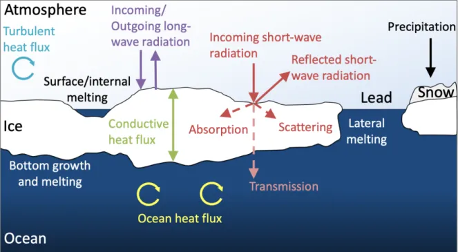
The simplified description of the ice-albedo feedback (Chapter 1) shows the relevance of ice-covered and ice-free areas for the surface energy budget in the Arctic Ocean (Fig. 2.1).

However, especially when it comes to the albedo of the ice surface, it is too simplistic to only consider the existence or absence of ice. Snow-covered ice provides the highest albedo (0.8 to 0.9), while snow-free ice is slightly darker (0.5 to 0.7), and freshly formed young ice is almost transparent, which results in a surface albedo close to that of the dark ocean (Curry et al., 1995). In this context, sea ice thickness is relevant as well. Thinner ice allows a larger fraction of solar energy to be absorbed by the ice or penetrate through to the underlying ocean (Nicolaus et al., 2012; Katlein et al., 2019). To predict and monitor what this increased energy input to the ocean means for primary productivity (Assmy et al., 2017), ocean heat deposition (Perovich et al., 2007; Pinker et al., 2014), and future development of sea ice in general, it is vital to observe sea ice thickness reliably. To comprehend the role and distribution of sea ice thickness in the Arctic, it is essential to understand how sea ice forms and how its thickness changes.

This chapter summarises how sea ice grows, evaluates processes changing its thickness, and describes its general distribution. It also provides information about different ice thickness measurement techniques, what they measure, and how to interpret and utilise the available data to investigate past, present, and future changes and variability in Arctic sea ice thickness.

2.1 Sea ice thickness distribution

The temporal development of sea ice thickness distribution, ∂IT D/∂t, is governed by three processes that are given by (Thorndike et al., 1975):

∂IT D

∂t =− ∂

∂H_ice(f ·IT D)

I

−div(#»v ·IT D)

II

+ Φ

III

, (2.1)

with f being the function for thermodynamic increase/decrease in ice thickness (H_ice), which depends on the location (x) and the time (t), represented in term I. Combining for the dynamic component of sea ice growth are the divergence in the ice drift velocity (#»v(x, t)), which describes the advection of sea ice (term II), and the redistribution function (Φ), which describes mechanical deformation (term III).

2.1.1 Thermodynamic components

Seawater freezes at approximately −1.9^◦C. The cold atmosphere cools the ocean surface, which gradually increases the density of the surface waters. As seawater approaches its freezing point, it penetrates downwards in the water column and is replaced by less dense, warmer water that is subsequently cooled by the atmosphere. This vertical mixing

(18)

Figure 2.1: Schematic showing relevant mechanisms of sea ice thermodynamics (adapted from Perovich and Richter-Menge (2009); Lepp¨aranta (2011)). Sea ice grows and melts forced by heat exchange with the atmosphere and the ocean and by radiation. Growth and melt occur at the upper and lower boundaries and in the ice interior (Lepp¨aranta, 2011).

reaches down to the halocline, which is the boundary layer between lower density surface and warm and saline deeper waters (Cottier et al., 2017). Depending on the atmospheric conditions, sea ice begins to grow as a thin layer in calm conditions, or as loose ice crystals (frazil ice) moving in the turbulent surface layer in windy conditions. Once the surface layer calms, frazil ice crystals consolidate to a solid layer. As sea ice continues to grow, congelation ice crystals form at the ice-water interface (Lepp¨aranta, 2011).

During the ice formation process, sea salt ions are rejected from the crystals and form brine at the ice-water interface (Petrich and Eicken, 2017). When ice growth continues, brine pockets can become enclosed into the newly formed ice, significantly altering the physical properties of the ice cover (Maykut and Untersteiner, 1971). Additional ice impurities influencing the physical properties of sea ice include incorporations of gases, organic matter, sediments, and pollutants (Rigor and Conoly, 1997; Dethleff et al., 2000;

Damm et al., 2018).

The growth rate of sea ice is determined by the energy balances at the sea ice bottom and surface (Fig. 2.1), which are coupled by conductive heat fluxes through the snow and ice layers (Petrich and Eicken, 2017). Sea ice forms an insulating layer at the ocean surface, limiting the exchange of heat between ocean and atmosphere. In general, sea ice growth at the bottom requires the surface air temperature to be below the freezing point of seawater and the conductive heat flux from the warmer ocean through the ice and to the atmosphere to be larger than the ocean heat input from below (Maykut and

(19)

2 Sea ice – Theoretical background 2.1 Sea ice thickness distribution

Untersteiner, 1971; Petrich and Eicken, 2017). As sea ice grows thicker, the insulating effect of the ice cover increases. It takes longer to transport heat from the ocean to the atmosphere, which is required to maintain the seawater freezing point and form ice at the ice-water interface (Lepp¨aranta, 2011). Hence, the rate of growth at the ice bottom is not only dependent on the physical properties of the inhomogeneous ice cover but also on its thickness.

The accumulation of snow on sea ice drastically increases the insulating effect of the ice cover. The thermal conductivity of snow is approximately one order of magnitude lower than that of sea ice and although snow only accounts for a small fraction of the total mass of sea ice, it further reduces its growth rate (Petrich and Eicken, 2017). Snow can also contribute to sea ice growth at the ice surface. Different types of ice form at the surface when snow is infiltrated by liquid water from precipitation, surface melt, or flooding and refreezes. Since flooding is the most common mechanism to form ice from snow, thick snow covers are required to submerge the ice into the ocean. Snow covers sufficiently thick to initiate this process are uncommon in the central Arctic and mostly occur in low-latitude seas on the northern hemisphere and in the Antarctic (Lepp¨aranta, 2011). However, recent studies have found that the impact of snow-ice on sea ice growth in the central Arctic may be increasing as more frequent storms bring heavy precipitation to the thinning central Arctic ice cover (Merkouriadi et al., 2017; Provost et al., 2017).

Ultimately, thermodynamic sea ice growth is limited. Based on the thickness and the composition of the snow and ice cover, the conductive heat fluxes from the ocean to the

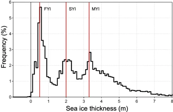
Figure 2.2: Example of sea ice thickness distribution measured in the Beaufort Sea in April 2008 (Hendricks, 2009). The three apparent modes indicate thicknesses of thermodynamically grown sea ice: first-year ice (FYI, 0.5 m), second-year ice (SYI, approximately 2 m) and multi-year ice (MYI, 3.3 m).

(20)

atmosphere are reduced, which slows the thermodynamic ice growth until an equilibrium thickness is reached (Maykut and Untersteiner, 1971; Lepp¨aranta, 2011). Theoretical estimates by Maykut and Untersteiner (1971) indicate that the equilibrium thickness of undeformed MYI can reach values between 3 and 4 m.

The second thermodynamic influence on ice thickness is melt, which, in general, occurs due to four different processes (Fig. 2.1). Solar and atmospheric heat fluxes lead to melting of snow and ice at the surface. In cases where the solar radiation is absorbed in the ice, it causes internal melting processes. When ocean heat fluxes exceed the conductive fluxes from the ocean to the atmosphere, sea ice starts to melt at the ice-water interface (bottom melt) or laterally at the ice edges in leads (Lepp¨aranta, 2011).

Figure 2.2 shows an example of the sea ice thickness distribution measured in the Beaufort Sea in April 2008 (Hendricks, 2009). The distribution displays the frequency of occurrence of different ice thickness values. The most frequently occurring thickness value (mode) is considered to be a measure for thermodynamically grown ice (Rabenstein et al., 2010; Haas, 2017). Three distinct modes are visible, indicating thermodynamically grown FYI (0.5 m), second-year ice (SYI, ice that has survived one summer melt season, approximately 2 m), and MYI (3.3 m). However, the example also shows the occurrence of ice thickness values considerably larger than the theoretical equilibrium thickness, which are the result of dynamic, and more specifically ice deformation processes.

2.1.2 Dynamic components

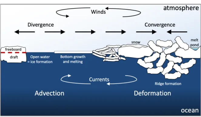
Dynamic effects on sea ice thickness can be divided into two main mechanisms (Fig. 2.3).

While divergence and advection are described by termII in Equation 2.1, the mechanical deformation of sea ice following convergence is given by the redistribution function, Φ (term III).

The divergence of the ice cover is the result of the prevailing wind fields and, to a lesser degree, ocean currents (Spreen et al., 2011). As long as ice motion is not prevented by obstacles or coastlines, sea ice drifts at approximately 1 to 2% of the mean wind speed (Spreen et al., 2011). However, multiple studies have shown that Arctic sea ice drift velocities are increasing (Spreen et al., 2011; Itkin and Krumpen, 2017), which is attributed to the general thinning of Arctic sea ice (Rampal et al., 2009), but also to the positive trend in wind stress caused by a shift in storm tracks (Hakkinen et al., 2008).

Divergence in the ice cover generates small openings, leads, and polynyas. Open water is exposed to the cold atmosphere and new ice forms. The removal of sea ice of a certain thickness by divergence results in zero thickness or a thin ice signal in the overall ice distribution (Haas, 2017). Regions where the continuous generation of open water areas leads to most of the Arctic’s sea ice formation are found on the shallow shelves of the Russian Arctic and specifically in the Laptev and East Siberian Sea. The prevailing wind fields transport newly formed ice northward and away from the coast, which opens large areas of open water where new ice can be formed (Timokhov, 1994; Krumpen et al., 2013).

The redistribution function, Φ, describes the deformation of sea ice in response to convergence (negative divergence) in the sea ice cover. Especially thin ice is susceptible to being transformed into thicker ice by deformation (Haas, 2017). Depending on the initial thickness and physical properties of the ice that is deformed, fracture mechanics,

(21)

2 Sea ice – Theoretical background 2.1 Sea ice thickness distribution

Figure 2.3: Schematic of the dynamic influences on the development of the sea ice thickness distribution (adapted from Haas and Druckenmiller, 2009). Sea ice thickness varies considerably and depends on various atmospheric and oceanic factors including wind, ocean currents, and sea and air surface temperatures (Meier and Haas, 2012).

the snow and ice interfaces, the energy of the deformation, and the scales on which these processes occur, sea ice deformation generates a wide range of thicknesses (Haas, 2017).

Mechanical changes in ice thickness are asymmetric, which means ice thickness increases mechanically but decreases only thermodynamically by melt (Lepp¨aranta, 2011), or by the advection of thinner ice to the specific region. The influence of deformation on the temporal development of the ice thickness distribution is the most challenging to quantify.

While thermodynamic ice growth is represented by the mode, the grade of deformation determines the tail of the overall thickness distribution and therefore governs its mean.

2.1.3 Sea ice thickness distribution in the Arctic

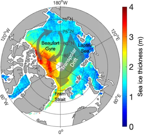
Changes in sea ice thickness at any given location and time are the result of a combination of the above-mentioned thermodynamic and dynamic processes. However, due to the large-scale atmospheric and oceanic circulation patterns in the Arctic, individual regions are dominated by either deformed MYI or thermodynamically grown younger ice (Zhang et al., 2000). The persistent atmospheric high pressure system over the Beaufort Sea is the main driver of the anticyclonic (clockwise) Beaufort Gyre and the Transpolar Drift system (Rigor et al., 2002, Fig. 2.4). Offshore-directed winds from the Siberian coast push newly formed, thin ice northward where it is incorporated into the Transpolar Drift. This process leads to continuous ice formation on the shallow Russian shelves and a dominance of thermodynamically grown young sea ice in this region (Krumpen et al., 2013). Ice not

(22)

Figure 2.4: January to April 2020 mean sea ice thickness from the ESA CCI-2 climate data record (Hendricks et al., 2018a), superimposed by schematics of the general Arctic sea ice drift patterns.

exiting the Arctic through Fram Strait is pushed towards the northern coast of Greenland and the Canadian Archipelago where it piles up and strongly increases its thickness mainly through deformation processes (Kwok and Cunningham, 2015). Most of this ice continues to circulate within the Beaufort Gyre and is usually much older and thicker than the ice passing along the Transpolar Drift (Rigor et al., 2002, Fig. 2.4).

The strength of both large-scale circulation regimes, the Beaufort Gyre and the Trans- polar Drift, is governed by the general wind-driven Arctic Ocean circulation and can be linked to the Arctic Oscillation (AO), which is described by surface level pressure anomalies over the Northern Hemisphere and especially the central Arctic Ocean (Thompson and Wallace, 1998). A positive AO phase is characterised by a negative surface pressure anomaly over the central Arctic Ocean, while a negative AO phase shows a positive pressure anomaly. The more cyclonic (counter-clockwise) motion of sea ice during a positive AO phase leads to increased transports of sea ice from the Russian shelves and a fast Transpolar Drift (Rigor et al., 2002). According to Rigor et al. (2002), the increasing ice formation in the Russian Arctic, a faster Transpolar Drift, and a coincidental slowing of sea ice motion in the Beaufort Gyre result in less ridging and recirculation of sea ice and should contribute to the thinning of sea ice during a positive AO phase. During a negative AO phase, ice from the Beaufort Gyre gets transported towards the eastern Arctic

(23)

2 Sea ice – Theoretical background 2.2 Key measurement techniques

much faster than during a positive AO phase. Due to the strengthened Beaufort Gyre circulation the ice exiting Fram Strait tends to be thicker than during a positive AO phase (Rigor et al., 2002). However, there is an ongoing debate whether the AO is the correct mechanism to describe variations in the general wind-driven Arctic Ocean circulation and the ensuing variations in sea ice drift speeds (Hakkinen et al., 2008; Rampal et al., 2009;

Spreen et al., 2011; Vihma et al., 2012).

Independent of the origin of observed variations in sea ice drift speeds, the dominant processes changing sea ice thickness, and the variations in the general circulation of sea ice in the Arctic, individual regions can be dominated by thermodynamically grown or dynamically deformed sea ice. Since the processes changing sea ice thickness strongly impact the physical properties of the respective ice, different measurement techniques are more suitable in different regions and for certain ice types than others.

2.2 Key measurement techniques

The large-scale distribution of sea ice thickness is one of the integral parameters for monitoring changes in the Arctic sea ice cover. Sea ice thickness varies strongly on local scales and its vertical extent is comparably small, which requires highly sensitive and accurate measurement techniques (Eicken et al., 2014). Beside the possibility of manually drilling sea ice to measure its thickness, most of the measurement techniques applied are indirect methods. This means that parameters related to the ice thickness are measured and sea ice thickness is inferred from these measurements (Haas, 2017). The most common methods used to measure or infer sea ice thickness, their limitations, and their main areas of application are presented in greater detail in the following. The most relevant methods for the studies presented in this dissertation are given a more detailed description in separate subsections.

The most accurate and direct way of measuring ice thickness is manually drilling the ice from the surface and measuring its thickness with a gauge (Haas and Druckenmiller, 2009). This method allows for the simultaneous observation of all thickness components:

ice freeboard and draft (combining for ice thickness), as well as snow thickness (Haas, 2017). While the accuracy of measuring ice thickness by drilling holes is unmatched, it is only possible in regions the observer can access. Once the observer is on the ice, it is tedious work and takes a lot of time. The enormous effort required limits the spatial extent of the measurements and restricts the validity of the results to a small area. A collection of ice thickness values measured with a drill is usually biased towards thicker ice, as very thin ice is hardly accessible on foot. Hence, manual drilling is mainly done to validate larger-scale measurements (Haas, 2017).

During shipborne expeditions, Arctic sea ice thickness is usually observed visually during the transit through the ice (recently based on the Arctic Shipborne Sea Ice Stan- dardization Tool, ASSIST/IceWatch protocol introduced by Hutchings, 2018). Ice frag- ments broken by a passing ship usually turn sideways against the hull and their thickness can be estimated visually or even with camera systems (Chapter 6). However, visual ice thickness measurements date back to the early 20th century and continue to be an integral part of Russian ice charting efforts managed by the Arctic and Antarctic Research

(24)

Institute (AARI). Sea ice thickness information is limited to the route of the ship and biased towards thinner ice that is easier to navigate.

Different configurations of autonomous measurement stations equipped with thermistor chains can infer sea ice thickness while drifting with the ice. Once the chain and its closely spaced thermistors are solidly frozen into the ice, vertical temperature profiles are measured. The vertical temperature gradients are very different in snow and ice and absent in the water and air columns close to the respective interfaces due to the differing thermal conductivities of the relevant layers. Using a satellite link to transfer the data, this technique allows for very accurate distinction of the interfaces between air, snow, ice, and water in quasi real-time. However, it is very limited spatially as it provides a point measurement and follows the drift path of a single ice floe. In addition, these thermistor buoys provide only thermodynamic changes of sea ice thickness and are prone to break during deformation events (Eicken et al., 2014).

2.2.1 Upward-Looking Sonar

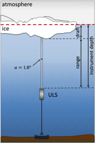
Upward-Looking Sonars (ULSs) are the primary source of long-duration sea ice draft data with high temporal resolution (Ross et al., 2016). They emit short pulses of acoustic energy in narrow beams and at frequencies of up to 2 Hz (Ross et al., 2016). The return signals are detected and the delay times between emitted and detected signal are precisely measured and converted into the distance between the instrument and the reflecting ice surface (range, Fig. 2.5). Additional information about the depth of the instrument un- derneath the water surface are required to derive sea ice draft. Usually ULS moorings are equipped with pressure sensors to record contemporary pressure data at the instrument.

In combination with surface pressure information, these data records provide accurate dis- tances between the instrument and the water surface. Taking sound velocity in seawater, possible current and tide-induced instrument tilts, and beamwidth biases into account, range is subtracted from the instrument depth to obtain sea ice draft (Ross et al., 2016, the relevant equations are provided in Chapter 3). Sea ice thickness can be inferred from the draft time series using a constant ratio between thickness and draft determined from drilling (Vinje and Finnekasa, 1986) or by assuming hydrostatic equilibrium. Following Archimedes’ principle, hydrostatic equilibrium assumes that the forces acting downward (gravity) and upward (buoyancy) on the observed ice are equally strong, which keeps the ice in a balanced position at the ocean surface. Based on this balance and information about snow depth and the densities of ice and snow, sea ice thickness can be derived (Eicken et al., 2014).

While all types of sonars are technically usable to derive sea ice draft, the Ice Pro- filing Sonar (IPS) was specifically designed for the application of deriving sea ice draft from acoustic data. IPSs have been mounted to submarines (Bourke and Garret, 1987;

Rothrock and Wensnahan, 2007) or oceanographic moorings (Fukamachi et al., 2003;

Hansen et al., 2013; Krishfield et al., 2014; Behrendt et al., 2015) in both the Arctic and Antarctic. Other sonar-based instruments, such as Acoustic Doppler Current Profilers (ADCPs), have also been used to derive sea ice draft time series (Shcherbina et al., 2005;

Banks et al., 2006; Hyatt et al., 2008).

(25)

Figure 2.5: Schematic of the measurement principle of upward-looking, or ice profiling sonars (adapted from (Ross et al., 2016)). The two-way travel time of the acoustic signal emitted from the ULS and reflected at the ice-water interface is calculated into distance between ULS and ice (range) and subtracted from the distance of the instrument to the air-water interface (instrument depth) to determine sea ice draft.

Submarine-mounted ULSs allow for long-range sea ice thickness transects in the regions where the submarines are operating and usually have to be corrected for seasonal variability in order to be compared to other data sets (Rothrock and Wensnahan, 2007).

Moored ULSs on the other hand provide continuous time series for single locations and for several years (Ross et al., 2016). State of the art IPSs are even deployed with a second mooring equipped with an upward-looking ADCP. Combining ice draft time series from the ULS and drift data from the ADCP allows for the derivation of spatial sea ice thickness series and detailed investigations of sea ice volume transports, especially when multiple ULS/ADCP mooring pairs are deployed along transects across known sea ice pathways (Hansen et al., 2013). However, the use of moorings is dependent on ice-free conditions during deployment and recovery, which limits their application to the seasonal ice zones, and data can not be obtained in real-time (see summary box for an overview of pros and cons of moored sonars).

(26)

Pros and cons: moored Upward-Looking Sonar Method: indirect

Accuracy: up to 0.05 m

Component measured: draft

Advantages: Disadvantages:

- high temporal resolution - spatially limited - year-round coverage - battery-powered

- thickness distribution - data access only after recovery of passing ice - deployment/recovery only

in ice-free conditions

2.2.2 Electromagnetic induction sounding

In contrast to ULS measurements of sea ice draft from below the ice, electromagnetic induction (EM) sounding is applied from above the sea ice and snow surface. The EM method takes advantage of different electrical conductivities of the investigated layers and was first applied for geophysical exploration (Kovacs et al., 1987). The EM device is equipped with a transmitter coil, which generates a primary electromagnetic field that penetrates through the low-conductivity ice and snow layers almost unaffectedly (Kovacs et al., 1987). While the conductivity of ice and snow ranges from 0 to 50 milli-Siemens per metre (mS m⁻¹), seawater conductivities typically reach values between 2400 and 2700 mS m⁻¹ (Haas et al., 1997). These values are highly dependent on the season and, in the case of the conductivity of sea ice, on the physical properties of the sampled ice (Haas et al., 1997). The penetrating primary electromagnetic field induces electric eddy currents in the seawater. The induced eddy currents generate a secondary field which penetrates upwards. The receiver coil in the EM device records the total electromagnetic field (primary and secondary field) and their differences in phase and amplitude (Kovacs et al., 1987; Hendricks, 2009). The proportionality between the strength of the secondary field and the distance from the coils to the conductive seawater surface is used to calculate the distance between the EM device and the ice-water interface, h_w (Keller and Frischknecht, 1966, Kovacs et al., 1987, Haas et al., 1997, Fig. 2.6 a)). Additional factors, such as signal frequency and coil orientation and spacing, also affect the received secondary EM signal (Haas, 2017). Due to the fact that the amplitude of the secondary field decreases exponentially with increasing distance between the conductive seawater surface and the receiver coil, state of the art EM devices used for ice thickness sampling are commonly operated at heights less than 20 m above the sea ice surface (Haas et al., 2009). These restrictions allow for two possible measurement setups that require different approaches to derive ice thickness.

The first setup uses ground-based EM devices (GEM), commonly built into a light- weight sledge, that are located directly on the ice or snow cover (offset between EM device

(27)

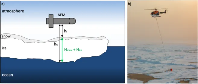
and surface has to be known) and effectively infer the distance between the air-ice and ice- water interface, the total ice thickness (Haas et al., 1997). The second setup uses airborne EM devices (AEM), that are towed from either a helicopter, fixed-wing aircraft (Kovacs et al., 1987; Multala et al., 1996), or even mounted to the bow of a ship (Haas, 1998) and infer the distance from their position to the ice-water interface (h_w). Radar or laser altimeters integrated into EM devices measure the distance from the instrument to the air-ice interface, h_i (Kovacs et al., 1987; Haas et al., 2009). This distance is subtracted from the EM-derived distance between the AEM and the ice-water interface to derive sea ice thickness (Fig. 2.6). Both the ground-based and the airborne approach therefore provide total sea ice thickness, including ice thickness,H_ice, and the thickness of the snow cover, Hsnow.

GEM measurements are obtained on foot or using snowmobiles, which limits the areal extent of the measurements significantly. However, parallel ground measurements of snow depth along the GEM surveys, using instruments such as the Magna Probe (Sturm and Holmgren, 2018), allow for reliable ice thickness data from these ground-based measurements. The spacing between individual measurements is dependent on the survey speed and the instrument configuration (Haas et al., 1997). For both of the approaches, it is important to ensure a large-enough distance between the EM device and any metallic parts to avoid disturbance of the EM field by other highly conductive media (commonly, a couple of meters for the GEM and approximately 60 m for the AEM). In addition to the spatial limitations, ice thickness distributions inferred from GEM measurements usually lack information about thin ice due to the limitations of sampling it on foot (Haas, 2004).

Figure 2.6: a) Schematic of the measurement principle of an airborne electromagnetic induction sounding (AEM) instrument (adapted from (Haas et al., 2009)). Total sea ice thickness (snow + ice thickness) is calculated from EM measurement inferred distance between the EM device and the ice-water interface,hw, and the laser altimeter measured distance between the EM device and the ice/snow surface, h_i. b) Airborne EM device (EM Bird) towed by a RV Polarstern helicopter in the Arctic (photo by Stefan Hendricks, Alfred Wegener Institute).

(28)

AEM measurements require considerable extra effort compared to the GEM measurements. Pilots have to fly the aircraft at very low altitudes to ensure that the distance between the AEM and the ice cover does not exceed 20 m. As for the GEM, towing the EM device is done to prevent interference from any conductive metal parts, but also to ensure safe flying altitudes for the aircraft. The airborne approach provides a significant increase in areal coverage compared to the ground-based setup but has a much larger footprint of two to four times the altitude of the EM device. Measurements are averaged over this footprint area, which is one of the reasons the maximum sea ice thickness is underestimated within each footprint (Eicken et al., 2014). While the EM-derived total thickness is within 0.1 m of drill hole measurements over level ice, it underestimates total ice thickness over deformed ice by approximately 40 to 50% (Pfaffling et al., 2007; Haas et al., 2009). Especially ridged ice consisting of ice blocks and connecting hollow spaces filled with seawater prevent accurate measurements of ridge keels (Haas et al., 2009).

In this context, improvements in EM sounding methods and especially the use of multi- channel sensors, which allow the detection of internal and bottom layers in different ice structures, are actively investigated to reduce the uncertainty over sea ice consisting of layers with different physical properties (Hunkeler et al., 2015; Haas, 2017).

Like moored ULSs, EM devices provide sea ice thickness distributions. However, EM- derived distributions are independent of sea ice motion and sampling is only dependent on weather conditions and the observer’s preferences. EM data are available immediately after sampling but lack the accuracy over ridged ice that is achieved using moored ULSs (see summary box for pros and cons of EM sounding).

Pros and cons: airborne and ground-based EM sounding Method: indirect

Accuracy: 0.1 m (level ice)

Component measured: total thickness (ice + snow) Advantages: Disadvantages:

- areal coverage (AEM) - areal coverage (GEM)

- accuracy over level ice - underestimation of deformed ice - thickness distribution - bias towards thicker ice (GEM)

over sampled area - limited by weather and accessibility - temporal coverage

2.2.3 Satellite remote sensing

Recent developments in satellite remote sensing of sea ice have resulted in a variety of open-access satellite sea ice thickness products (Sallila et al., 2019). Satellite retrievals of sea ice thickness are based on two main measurement principles. Active satellite remote sensing uses the active emission of an electromagnetic signal from the satellite and the

(29)

recording of the respective reflected or backscattered signal from the ice and ocean surface to derive a sea ice related parameter that can be converted into sea ice thickness (Spreen and Kern, 2017). Passive satellite remote sensing of sea ice thickness is carried out using radiometry, which uses the fact that the Earth itself emits electromagnetic radiation.

These received radiative signals are used to infer sea ice thickness (Spreen and Kern, 2017).

Since the 1990s, various different configurations of altimeters (active) and radiometers (passive) have been deployed with satellites, with altimetry being the most commonly applied method for the derivation of various satellite sea ice thickness products today (Sallila et al., 2019).

The focus of the study presented in Chapter 4 is on the validation and application of the longest available satellite sea ice thickness data set, which consists of combined data from two different satellite altimetry missions. The following section will therefore present a basic summary of the application of satellite altimetry for the derivation of sea ice thickness but also touch on the radiometric approach, to introduce the second satellite sea ice thickness product investigated. This second product combines the advantages of active and passive satellite remote sensing for an improved satellite sea ice thickness product.

Satellite altimeters used to derive sea ice thickness measure different forms of the fraction of the ice that protrudes from the ocean – freeboard. The determination of freeboard is strongly dependent on and requires knowledge of the physical properties of snow, ice, their respective surfaces, and the sea surface height. Due to the comparably large footprints of the used altimeters, the correct determination of sea surface height over almost closed ice covers is challenging. Open water areas, required to detect the sea surface, usually occur on comparably small spatial scales that can not be resolved (Spreen and Kern, 2017) and available mean sea surface height data sets have to be used instead (Sallila et al., 2019). Like the determination of the sea surface height, deriving the height of the snow surface is achieved using different approaches and data sets (Sallila et al., 2019). While some configurations of radar altimeters that are assumed to fully penetrate the snow cover provide ice freeboard, others together with laser altimeters determine the height of the total freeboard, including snow and ice freeboard (Spreen and Kern, 2017).

As summarised in Sallila et al. (2019), the most commonly used products rely on different algorithms and assumptions to detect the desired interface and sea surface height (Kwok et al., 2009; Laxon et al., 2013; Kurtz et al., 2014; Ricker et al., 2014; Tilling et al., 2018). However, the strong annual changes in the physical properties of ice and snow even prevent the detection of these interfaces completely during periods of surface melt (Ricker et al., 2017; Hendricks and Ricker, 2019a). This is why satellite altimeter sea ice thickness data are usually only available for the winter months, when the air-snow or snow- ice interface can be detected. Once freeboard is determined, it is converted into sea ice thickness. Like for the above-mentioned ULS calculations, this conversion is based on the assumption of hydrostatic equilibrium and auxiliary information of snow and ice density and snow depth (Spreen and Kern, 2017). While the ULS-based method to derive sea ice thickness utilises the submerged larger fraction of ice, the draft, for the conversion to sea ice thickness, the altimeter approaches use the smaller fraction, freeboard. Due to the small freeboard/thickness ratio even small errors in freeboard strongly effect the accuracy

(30)

of the final sea ice thickness estimate (Eicken et al., 2014). It is therefore vitally important to acquire reliable information of snow and ice density and snow depth that is not only required for the determination of freeboard but also for the conversion of freeboard into sea ice thickness. Since snow depth and snow and ice densities are not routinely measured, current satellite sea ice thickness products have to rely on assumptions and estimates for these parameters, which increases the uncertainty of the final sea ice thickness product even further (Spreen and Kern, 2017; Hendricks and Ricker, 2019b).

The above-mentioned longest available satellite-derived sea ice thickness climate data record is a product of the European Space Agency’s (ESA) Climate Change Initiative Phase 2 (CCI-2). Combining radar altimeter-derived sea ice thickness data from the Environmental Satellite (ENVISAT, Hendricks et al., 2018c) and from CryoSat-2 (CS2, Hendricks et al., 2018a), this product provides monthly mean sea ice thickness from 2002 onwards. The initial daily orbit data is interpolated to a 25 km resolution grid. However, due to the limitations of freeboard retrieval during ice and snow melt and the resulting high moisture content at the ice surface, data is only available from October through April (Ricker et al., 2017; Hendricks and Ricker, 2019a).

The second data product utilised here is a merged product combining CS2 altimeter- derived sea ice thickness and radiometer-derived sea ice thickness from the Soil Moisture and Ocean Salinity (SMOS) satellite (Ricker et al., 2017). SMOS sea ice thickness is derived using radiometer measurements of the thermal microwave radiation emitted by a closed ice cover during freezing conditions (Kaleschke et al., 2010). This passive remote sensing method relies on the fact that different media posses different radiative properties.

In terms of sea ice thickness derivation, the different radiative properties of seawater and sea ice of different thicknesses are utilised (Spreen and Kern, 2017). The specific parameter observed by the SMOS radiometer is the surface brightness temperature, which is dependent on ice and seawater temperatures and their respective emissivities (Kaleschke et al., 2010). It has been shown that the SMOS ice thickness retrieval algorithm, based on a combined thermodynamic and radiative transfer model, is best suited to retrieve sea ice thickness values of ice thinner than 0.5 m (Kaleschke et al., 2012; Tian-Kunze et al., 2014). While uncertainties of SMOS sea ice thickness are lower over thin ice compared to radar altimeter retrievals, uncertainties increase exponentially for ice thicker than 0.5 m (Tian-Kunze et al., 2014). The complementarity of the relative uncertainties of CS2 and SMOS sea ice thickness shown by Kaleschke et al. (2015) was used by Ricker et al. (2017) to develop a merged sea ice thickness product (CS2SMOS). This merged product not only reduces sea ice thickness uncertainties by prioritising the lower uncertainty data set but also increases the temporal resolution of satellite-derived sea ice thickness data from monthly to weekly (Ricker et al., 2017).

For the satellite sea ice thickness validation study presented in Chapter 4, the ESA CCI-2 radar altimetry-based and the merged CS2SMOS product are selected, as they provide the longest available record and the highest temporal resolution of the available gridded sea ice thickness products, respectively. Despite the improvement in temporal resolution provided by the merged CS2SMOS product, temporal coverage is one of the main limitations of satellite-derived sea ice thickness data in general. Both data products only provide data from October through April with no sea ice thickness data available

(31)

during the Arctic summer season. Additionally, these data products provide gridded averages of sea ice thickness (Ricker et al., 2017; Hendricks and Ricker, 2019a,b). Sea ice thickness distributions especially on scales smaller than their 25×25 km grids are not available and thermodynamic and dynamic thickness changes that occur on these small spatial and short temporal scales are not represented at all. The uncertainty of the gridded mean values of sea ice thickness are given for each grid point (Hendricks and Ricker, 2019a) and vary substantially for different regions and months. As an example, the Arctic-wide average of ESA CCI-2 sea ice thickness uncertainty is approximately 0.65 m (in April, see summary box for pros and cons of satellite remote sensing).

Pros and cons: satellite remote sensing Method: indirect

Uncertainty: satellite product specific e.g. ESA CCI-2: 0.65 m (Arctic mean April) Component measured:

freeboard (altimeter), brightness temperature (SMOS) Advantages: Disadvantages:

- Arctic-wide data - temporal resolution - weekly resolution - temporal coverage

(merged CS2SMOS) (no summer data)

- small-scale features not resolved - high uncertainty

2.2.4 Conclusion

The comparison of ULS, EM and satellite-based methods to derive sea ice thickness shows the requirement for further development and improvement of sea ice thickness measurements. Each of these methods has at least one characteristic that is superior to other methods and more suitable for specific applications. However, no method currently available provides sufficient spatial resolution and Arctic-wide coverage paired with high temporal resolution and year-round coverage to observe the complex changes of sea ice thickness and its distribution comprehensively. In the absence of an overall sufficient sea ice thickness data set, it is necessary to improve and combine data from different measurement techniques and regions and find solutions to connect these data sets. Therefore, the studies within this dissertation aim to contribute to the extension of existing data sets and the improvement of satellite sea ice thickness products but also combine available data, models, and additional tools for the investigation of ongoing sea ice thickness changes and variability in the Arctic.

(32)

(33)

3 Sea ice draft from upward-looking Acoustic Doppler Current Profilers: an adaptive approach, validated by Upward-Looking Sonar data

Currently under review at Cold Regions Science and Technology Belter, H. J.¹, T. Krumpen¹, M. A. Janout¹, E. Ross², and C. Haas¹

1Alfred Wegener Institute, Helmholtz Centre for Polar and Marine Research, Bremer- haven, Germany

2ASL Environmental Sciences Inc.

Author contributions

HJB processed the 2014/2015 ULS data and together with MAJ developed the method to derive sea ice draft from upward-looking ADCP data. HJB also conducted the statisti- cal analysis and comparison of ULS and ADCP-derived draft and wrote the manuscript.

TK, MAJ and CH provided guidance and important comments during the writing, edit- ing, and review of the manuscript. Apart from their contributions to the writing of the manuscript MAJ deployed and recovered the ADCP and ULS moorings and ER processed the 2013/2014 ULS data. ER also provided support during data processing.