Strong coupling and non-Markovian effects in the statistical notion of temperature
Camilo Moreno*and Juan-Diego Urbina
Institut für Theoretische Physik, Universität Regensburg, D-93040 Regensburg, Germany
(Received 14 December 2018; revised manuscript received 13 March 2019; published 27 June 2019) We investigate the emergence of temperature T in the system-plus-reservoir paradigm starting from the fundamental microcanonical scenario at total fixed energy E where, contrary to the canonical approach, T =T(E) is not a control parameter but a derived auxiliary concept. As shown by Schwinger for the regime of weak couplingγbetween subsystems,T(E) emerges from the saddle-point analysis leading to the ensemble equivalence up to correctionsO(1/√
N) in the number of particlesNthat defines the thermodynamic limit. By extending these ideas for finiteγ, while keepingN→ ∞, we provide a consistent generalization of temperature T(E, γ) in strongly coupled systems, and we illustrate its main features for the specific model of quantum Brownian motion where it leads to consistent microcanonical thermodynamics. Interestingly, while thisT(E, γ) is a monotonically increasing function of the total energyE, its dependence withγ is a purely quantum effect notably visible near the ground-state energy and for large energies differs for Markovian and non-Markovian regimes.
DOI:10.1103/PhysRevE.99.062135
I. INTRODUCTION
In the context of statistical physics there are two ways to explain how a system A acquires a property associated with the thermodynamic notion of temperature [1,2]. In the first approach, one considers the system as weakly coupled with a thermal bathB that is initially in a canonical state at temperature T. If we wait long enough, A will equilibrate (in the sense of stationarity of macroscopic observables) and acquire itself a canonical distribution at the same T. Here, therefore, the idea of temperature is preassumed from the beginning. In the second approach, one considers instead that the global systemA+B is in a microcanonical distribution at total energy E (we agree with Refs. [3–5] that this is the conceptually foundational starting point to understand the meaning of temperature). HereAandBequilibrate due to the presence of aweakinteraction term, and the temperature will emerge as a parameter that fixes the condition of equilibrium.
The temperature T =T(E) is then a derived rather than a fundamental quantity.
As has been shown when going beyond the assumption of weak interactions, for strongly coupledAandB deviations from the standard thermodynamics emerge [6–9], as well as problems defining local temperature [10–13]. Also, the equivalence between the microcanonical and the canonical approach does not hold, correlations between system and bath become important, and the system is nonextensive by nature [14–16]. In this context it is well known that when A is strongly coupled to a thermal bath the long-time steady state of the system, contrary to the weak coupling scenario, does not take the Boltzmann form, neither in the open-quantum system approach [17–19], in the global closed thermal state scenario [20], nor in the pure state setup [21,22].
*camilo-alfonso.moreno-jaimes@stud.uni-regensburg.de
Here we will provide a consistent definition of temperature T in the system-plus-bath scenario with arbitrary coupling strength γ by starting with a global microcanonical state at energy E and generalizing the saddle-point analysis of ensemble equivalence pioneered by Schwinger [23,24].
The paper is organized as follows. In Sec.IIwe review the relevant aspects of the emergence of temperature in the weak coupling scenario, then in Sec. III we generalize this idea to the finite coupling case, and as an experimental relevant application, we will present the main features of this definition of temperatureT(E, γ) in the solvable case of quantum Brow- nian motion. We give some general conclusions in Sec.IVand an outlook overview in the last section, Sec.V.
II. THE STATISTICAL EMERGENCE OF TEMPERATURE FROM A SADDLE-POINT CONDITION
Let us first review the weak coupling case by consid- ering two many-body systems A andB with Hamiltonians HˆA and ˆHB that in isolation have fixed energies EA,EB. When brought into weak thermal contact allowing them to interchange energy through a small interaction term such that Eint(γ)EA+EB, in equilibrium the resulting global state is microcanonical,
ρˆAB= δ(E−HˆAB)
GAB(E) , (1) with total energy E=EA+EB+O(γ). Here ˆHAB =HˆA+ HˆB+O(γ) acts in HA⊗HB and GAB(E)=TrABδ(E− HˆAB) is the microcanonical partition function, the central quantity connecting statistics and thermodynamics through the Boltzmann equation
S(E)=KlogGAB(E), (2) for the thermodynamic entropy S(E), where K is the Boltz- mann constant.
The emergence of temperature in this microcanonical, weak-limit scenario starts with writing the density of states, expanding the operator-valued Dirac delta function [25], as
GAB(E)=TrAB δ(E−HˆAB)
= 1 2π
∞
−∞dτeiEτTrAB[e−iτHˆAB], (3) whereτ is an integration variable with units of inverse energy.
Defining TrAB[e−iτHˆAB]=ZAB(iτ), Eq. (3) takes the form GAB(E)= 1
2π ∞
−∞dτeiEτelogZAB(iτ), (4) with an associated actionφ:
φ(E, τ)=iEτ +logZAB(iτ)
=iEτ +logZA(iτ)+logZB(iτ), (5) where the decomposition ZAB=ZA+ZB with ZA = TrA[e−iτHˆA] and ZB=TrB[e−iτHˆB] is possible because the interaction term is small enough to be neglected. Following an idea due to Schwinger [23], for a large number of degrees of freedomN→ ∞, the quantitiesE and logZAB are large (allowing rapid oscillations in the exponential), and we can solve the integral in Eq. (4) using the saddle-point approximation (SPA). The saddle-point condition
d
dτφ(E, τ) τ=τ∗
=! 0 (6) admits an analytical continuation over the lower half of the complex τ plane where we find the sole saddle pointτ∗ =
−iβ, withβsatisfying iE+i d
dβ logZA(β)
β=iτ∗+i d
dβ logZB(β) β=iτ∗
=! 0. (7) By interpreting the real solutionβ =1/KT as the inverse temperature and Zi(β)=Zi(iτ∗) as the canonical partition function, then ¯Ei= −ddβlogZi(β) is the mean internal energy of each subsystem, and the relation
E =E¯A(β =iτ∗)+E¯B(β =iτ∗) (8) gives a condition on how the total energy is distributed be- tween systemsAandB when they are brought into contact.
This microscopic analysis is thus used as the definition of both thermal equilibrium and the inverse temperature that fixes this condition.
Before we make this microscopic construction complete and see howβ(E) can indeed be interpreted as the thermo- dynamic temperature, we find it important to complete the analysis of Ref. [23] by discussing the regime of validity of the SPA as well as the behavior of the error terms in the thermodynamic limit. In order to bring Eqs. (4) and (5) to the form required by the SPA, we consider first the situation where the total number of particles N=NA+NB and energyEare distributed in such a way that the ratiosνA = NA/N, νB =NB/N,u=E/N converge to nonzero constants whenN → ∞. Within this usual definition of thermodynamic limit applied to both subsystems A,B, the ratios logzA =
NA−1logZA,logzB =NB−1logZB also converge to finite val- ues, and the phaseφ(E, τ) in Eq. (5) takes the form
φ(E, τ)=N[iuτ+νAlogzA(iτ)+νBlogzB(iτ)]. (9) Substitution of Eq. (9) brings Eq. (4) to the form suitable for SPA and rigorously identifies the large parameter as N.
From the general theory we then conclude that the error in the evaluation ofGAB(E) in Eq. (4) by means of SPA is of order O(1/√
N), and it remains bounded as long asd2φ/dτ2 =0.
With these observations in mind, let us use Eqs. (2) and (4) with the solution established by Eq. (7) to obtain
GAB(E)=eS(E)K = eβE+logZAB(β) 2π∂2log∂βZAB2 (β)
[1+O(N−1/2)], (10) which by introducing the Helmholtz free energy F(β)=
−1β logZAB(β) immediately gives the well-known thermody- namic relation [24]
S(E)/K=βE−βF(β) ⇐⇒F =E−T S(E). (11) If there exist many solutions to Eq. (6) over the imaginary τ axes, say,τ1∗= −iβ1, τ2∗ = −iβ2 withS1(E)>S2(E), we must choose the solutionτ1∗in Eq. (10) in accordance with the principle of maximum entropy and neglecting exponentially small corrections∼eS2−S1.
In the approach of Schwinger, the focus of the SPA analysis was to provide a way to justify the ensemble equivalence as follows. Following a similar procedure as the one leading to Eq. (4), we write the microcanonical density matrix ˆρAB in Eq. (1) as
ρˆAB(E)= 1 2πGAB(E)
× ∞
−∞dτeiτEelogZAB(iτ)e−iτHˆAB
ZAB(iτ), (12) where we have multiplied and divided byZAB(iτ). The expec- tation value of an observable ˆOacting on the global system can then be written in the form
OˆE = 1 2πGAB(E)
∞
−∞dτeiτEelogZAB(iτ)Oˆiτ, (13) where Oˆ iτ=TrAB[ ˆOe−iτHˆAB/ZAB(iτ)]. In the thermody- namic limit, provided Oˆiτ varies slowly with respect to τ [24], the integral in Eq. (13) can also be solved by SPA, resulting in Oˆ E ≈ Oˆ β(E), where β(E) is the solution of Eq. (7). This is the meaning of equivalence of ensembles, according to Schwinger, in the weak coupling approach. Note that Eq. (13) is a mathematical identity which relates the expectation value of a global observable ˆOcalculated in the microcanonical equilibrium with the quantityOˆ iτ, which in the thermodynamic limit will give the canonical expectation value of the observable evaluated at the inverse temperature β(E). This identity then does not refer to any dynamical process of equilibration in time. The topic of dynamical equi- libration or relaxation goes beyond the formalism developed in this paper. In summary, Eq. (8) establishes a relation of energy equilibrium between two many-body systems. The condition of equilibrium is fixed by the inverse temperature
β coming from the SPA analysis of Eq. (6) in the thermody- namic limit. We establish this limit considering, for example, a many-body global system A+B with a constant energy per particle, where the total energy scales with the number of particlesN. In that case the thermodynamic limitN→ ∞ gives the relation Eq. (10). It is satisfactory to see how the SPA analysis formalizes the difference between the scenario of mutual equilibrium, where both subsystems are macroscopic and the temperature emerges from the distribution of the total energy where both systems get a finite fraction, and the bath scenario whereνA =0 in Eq. (9) and the temperature of the subsystem is simply inherited from the temperature of the bath. In this last scenario the functionelogZA(iτ)=ZA(iτ) is smooth and does not participate of the SPA condition.
III. FINITE COUPLING REGIME
After this revision of the key aspects of the emergence of temperature in composite weakly interacting systems, we now proceed to extend these ideas to systems with non-negligible interaction Hamiltonian ˆHint. The key point that allow for this generalization is that the SPA analysis that naturally leads to the concept of temperature is not restricted to γ →0 at all, and in fact its only requirement is consistency with the thermodynamic limitN → ∞. While the global equilibrium state in the case of finite interaction energy is
ρˆAB= δ(E−HˆA−HˆB−Hˆint)
GAB(E) , (14) and the density of states is still given by Eq. (4), nowZAB(iτ) cannot be unambiguously decomposed in general in terms of the bare Hamiltonians ˆHA and ˆHB [26]. However, our key observation is thatas long as we can solve the integral in Eq. (4) by SPA, the resulting real solution forβ, which now depends not only on the total energy E but also on the parameters of the interaction, characterizes the condition of thermal equilibrium betweenAand B, thus providing the statistical definition of temperature for systems with finite coupling. To support this claim we will now study the consistency and consequences of this definition in a solvable example.
As a specific microscopic model that allows for almost full analytical treatment and remains of high experimental relevance, we consider now a microcanonical modification of the widely used open-system approach to quantum Brownian motion (QBM) [27]. HereAconsists of a quantum harmonic oscillator linearly coupled to a bath B of N noninteracting harmonic oscillators. The total Hamiltonian reads
HˆAB = pˆ2 2m+1
2mω20qˆ2 +1
2 N n=1
pˆ2n mn
+mnω2n
ˆ qn− cn
mnωn2
ˆ q
2
, (15) where ˆpand ˆqare momentum and position operators, respec- tively, of the coupled harmonic oscillator with bare frequency ω0 and massm, and ˆpn,qˆn the momentum and position oper- ators, respectively, of thenth bath oscillator with frequency ωn and mass mn coupled with the central system through characteristiccnfixed for a given model of the bath. The bath
and interactions are characterized by the bare and coupled spectral densities that distribute the frequenciesωnlike
I(ω)=π N
n=1
δ(ω−ωn)=κω2e−ω/ωD, (16a)
J(ω)=π N n=1
cn2
2mωnδ(ω−ωn)=mγ ωe−ω/ωD, (16b) with cutoff Drude frequency ωDand so-called damping pa- rameter γ, which is a function of the parameters c2n char- acterizing the system-bath coupling strength. The parameter κ is a characteristic of the bath with units ofω−3 such that ∞
0 dωI(ω)/π =N.
In order to use Eq. (4), we constructZAB(iτ) of the QBM model by analytical continuation of the Matsubara frequen- ciesνn= 2hi¯πτnfrom the known result [28], to get
ZAB(iτ)=ZB(iτ)
× 1 hiτω¯ 0
∞ n=1
νn2(ωD+νn) ω20+νn2
(ωD+νn)+νnγ ωD
. (17) Here the imaginary temperature partition functionZB(iτ) of B, using the spectral density from Eq. (16a), reads
logZB(iτ)= −iτE0+2κζ(4)
( ¯hiτ)3 , (18) whereE0=3κhω¯ D4 is the zero point energy of the bath, and ζ(x) is the Riemann zeta function. In this way we arrive at
logZAB(iτ)=logZB(iτ)+log ˜Z(iτ), (19) where the effective ˜Z, related to the coupled harmonic oscilla- tor, has an explicit form in terms of Gamma functions[28],
Z˜(iτ)= hiτω¯ 0( ¯hiτλ1/2π)( ¯hiτλ2/2π)( ¯hiτλ3/2π) 4π2( ¯hiτωD/2π) ,
(20) withλ1, λ2 andλ3 being the roots of the polynomial expres- sion in νn that appears in the denominator of Eq. (17) and which carry the dependence onγ , ωD, andω0.
Interestingly, as shown in Ref. [29], for systems that have an interaction that involves only relative coordinates, like in Eq. (15), theclassical partition function does not depend at all on the coupling
logZAclassicB (iτ)=logZBclassic(iτ)+logZAclassic(iτ), and therefore the temperatureβ is independent ofγ, regard- less how strong the interaction is. This means that for the model in Eq. (15)the dependence of the temperature on the coupling strength is purely a quantum effect.
Before going further we make an important remark. Since our model consists of a single harmonic oscillator (system A) linearly coupled to many harmonic oscillators (systemB), we find here the situation where the SPA analysis requires νA =0 as discussed in the last part of Sec. II. Since the function ˜Z in Eq. (19) encloses the effect ofboththe single harmonic oscillator plus interaction terms, we must subtract from Eq. (19) the term logZA(iτ) due to the bare central
oscillator, meaning that we are considering ZA(iτ) smooth enough not to let it participate in the SPA analysis of Eq. (4).
With this in mind we now use Eqs. (4), (18), and (19) to identify the action
φ(iτ)=i(E−E0)τ +2κζ(4)
( ¯hiτ)3 +log ˜Z(iτ)−logZA(iτ).
(21) Solving the integral in Eq. (4) by SPA, using the saddle- point condition in Eq. (6), and again, looking for real solutions β=iτ∗, we get
E−E0−6κζ(4)
¯ h3
1 β4 = 1
β −hω¯ 0
2 coth βhω¯ 0
2
+ h¯ 2π
ωDψ(1+h¯βωD/2π)
− 3
i=1
λiψ(1+hβλ¯ i/2π)
, (22) where we have inserted Eq. (20) into (21). Note the subtracted energy of the bare oscillator h¯ω20coth (βh¯2ω0). Here ψ(x)=
d
dxlog(x) denotes the Digamma function.
Equation (22) establishes the equilibrium relation for the total energyE between systemBand the interaction energy, where the left-hand side is related with the energy of the bath and the right-hand side accounts for the energy of interaction.
In the regime whereγ =0 the right-hand side of Eq. (22) is zero. In this case the derived temperature is given by the bath.
This is the common scenario in the weak-coupling canonical approach, where the central system acquires a temperature given by the constant temperature of the canonical thermal bath. Here we will show that an interaction term that couples linearly the system with each degree of freedom of the bath gives rise to an interaction energy which affects the resulting equilibrium temperature.
The divergences affecting Eq. (22) forωD→ ∞arise from the well-known [30] divergences of the ground-state energy of the coupled harmonic oscillator0,
0= h¯
2π[λ1log(ωD/λ1)+λ2log(ωD/λ2)+λ3log(ωD/λ3)], but are readily renormalized by ˜Z×eβ0 to obtain a global zero ground-state energy. The new relation (22) for renormal- ized energy finally reads
E−6κζ(4)
¯ h3
1 β4 = 1
β+ h¯
2π{ωDψ(1+h¯βωD/2π)−ωDlogωD}
− h¯ 2π
3 i=1
[λiψ(1+h¯βλi/2π)−λilogλi]
−hω¯ 0
2 coth βhω¯ 0
2
+hω¯ 0
2 , (23)
where we have made use of the Vieta relationλ1+λ2+λ3= ωD [28]. The solution of Eq. (23) for β (fixing the energy equilibrium condition for our model) accordingly defines the inverse temperature in the finite coupling regime. This solutionβ(E, γ), our main result, depends on the interaction γ and the total energyE, but also the bath parametersκ and
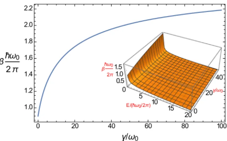
FIG. 1. Inverse temperature β(γ) for given values κω30= 5, ωD/ω0=10, andE/(¯hω2π0)=0.2, showing the increase ofβwith γ near the ground-state energy. Inset shows the variation ofβ(E, γ) for a large range of energies, showing a monotonic decrease withE. ωD. Coming back to the issue of SPA versus weak coupling expansions, we stress again that in a model where the total energy E scales with the number of particlesN, in solving Eq. (4) by SPA we are neglecting terms ofO(1/√
N), which is justified in the thermodynamic limit for large number of particles [24]. Still, the SPA approximation does not depend on any perturbative expansion of the interaction parameterγ, and thus our results are valid beyond the weak-coupling limit.
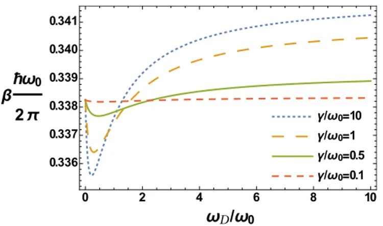
In Fig. 1 we show the numerical solution β(E, γ) of Eq. (23) for given values ofκandωDand for energy near the renormalized ground state where quantum effects are more visible. A clear variation of the temperature as a function of γ is observed, showing that the interaction energy has a sensible effect in the derived temperature. In the inset of Fig.1 can be observed thatβ is a monotonous function of the total energyE. From Eq. (23), and using the asymptotic expansion of Digamma functions, we obtain that for β→ ∞,E →0, as expected. For large energies the change of β with γ is less evident but still can be appreciated in Fig.2. Remarkably in this regime the behavior of β withγ is modulated by the tuning parameterωD/ω0, which also quantifies the degree of memory of the bath or non-Markovianity [31]. This surprising connection between the dependence of the temperature on
FIG. 2. β(γ) for parametersκω03=5 andE/(h¯2ωπ0)=10, show- ing the increasing ofβin the Markovian regime and its change of behavior in the non-Markovian case.
FIG. 3. β(ωD) for parametersκω03=5 andE/(hω¯2π0)=10, show- ing the explicit dependence ofβwith the Drude frequency and its change of behavior from Markovian to non-Markovian regime.
the coupling and the timescale 2π/ωDassociated to memory effects in the environment is also shown by the explicit dependence ofβon the Drude frequency in Fig.3.
We can provide a physical interpretation of the peculiar de- pendence ofdβ/dγon the Drude frequencyωDfor our results in the following way: In theMarkovian regimeFig.2suggests that the action from the bath on the central system mostly determines the energy equilibrium condition: the energy-flow follows the natural direction from bath to system to reach equilibrium. Moreover, it can be shown that the right-hand side of (23) grows withγ in this regime. That explains the growing behavior ofβwithγ in this case. On the other hand, in thenon-Markovian regimeFig.2suggests that is the action from the system on the bath which determines the equilibrium condition: in this case the energy-flow direction goes from system to bath. Also, it can be shown that the contribution of the right-hand side of (23) in this case follows a decreasing or increasing behavior as a function ofγ depending on the particular range of values ofωD/ω0within the non-Markovian regime. This is reflected in the peculiar behavior appearing in Fig.2.
We want to emphasize that the results obtained here go beyond any finite-order expansion around the weak-coupling scenario. Figure4 shows the contrast between the solution for temperature obtained in the first-order expansion forγ in Eq. (23) and that obtained from the full expression. The char- acteristic saturation behavior clearly indicates the breakdown of any finite-order approximation in powers ofγ.
Having obtained the inverse temperatureβ(E, γ) we can calculate thermodynamic potentials for finite coupling. We start with Eq. (10), from which the entropy of the global system in the limitN → ∞can be calculated by
logZAB(β)=S(E)/K−βE. (24) Recognizing thatβ(E, γ) is a function ofE, we get
1 K
∂S
∂E =β+ ∂β
∂E
E+ ∂
∂β logZAB
, (25)
FIG. 4. Contrast between the temperature solution at first order expansion inγ and the full results, showing the characteristic sat- uration behavior of the full result in contrast with the first order perturbative expansion inγ.
and since ∂β∂ logZAB = −E, we finally obtain the thermody- namic relation
1 K
∂S
∂E =β(E, γ). (26) Following Ref. [32] we may also calculate the entropy for the coupled oscillator as
SA
K =log ˜Z(β)−β ∂
∂β log ˜Z(β), (27) where ˜Z is taken from Eq. (20) and evaluated at the solution β(E, γ) given by the SPA condition. The term−∂β∂ log ˜Z(β) is the thermodynamic mean energy of the coupled oscillator evaluated atβ(E, γ).
Figure5illustrates the behavior ofSAas a function of the total energyE for various values of the couplingγ. As can be observed,SAis a positive quantity that becomes zero forE = 0, in nice accordance with the third law of thermodynamics.
The entropy is also a monotonically increasing function ofE andγ. This latter feature accounts for the decrease in purity of the reduced density matrix TrBρˆABwith increasingγ.
Finally, let us consider the finite coupling version of the ensemble equivalence. Whenever the solution of the integral
FIG. 5. Subsystem entropy SA(E, γ) for parameters κω30=5 andωD/ω0=10. The entropy of the subsystemAis parametrically larger when the system-dependent damping γ is large and also increases with the energy and becomes zero forE=0, in accordance with the laws of thermodynamics.
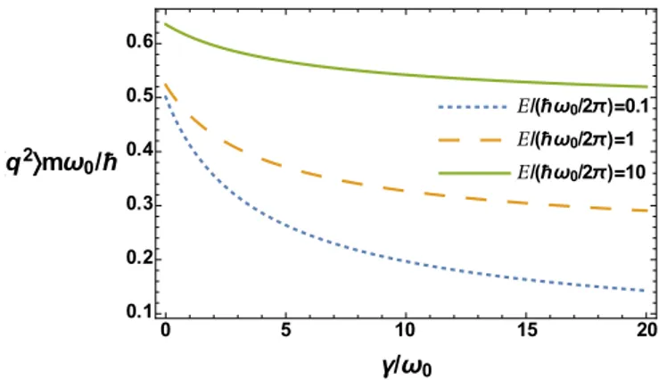
FIG. 6. q2(γ) for parameters κω03=5 andωD/ω0=10. As expected the particle gets more localized with increasingγ, and its squared position expectation value increases withE.
in Eq. (13) is justified by SPA, the saddle-point condition will give a relation between the expectation value of any smooth operator calculated in the microcanonical ensemble and the one evaluated in the canonical case, but for a temperature given by the solutionβ(E, γ)in the finite coupling regime. The same considerations also hold for the reduced density matrix describing the subsystemA, and, in that case, the relation for the expectation value of an observable ˆOAis given as
OˆAE ≈ OˆAβ(E,γ), (28) which provides the sought extension of the equivalence of ensembles for systems with finite coupling in the thermody- namic limit. Accordingly, in Fig.6we show the expectation value of the squared position operator of the coupled oscillator evaluated at the solution β(E, γ). As expected q2 grows with the energyE, and the particle is getting more localized with the increase of the damping parameter γ, as the bath monitors the position of the central particle [33].
It is interesting to note that a similar behavior of the entropy and the expectation value of the squared position with respect toγin the QBM model is found in the canonical thermal bath approach [28,32]. This is actually a nontrivial result due to the fact that our microcanonical thermodynamics is based on β(E, γ), which is a SPA condition solution that involves γ. One could imagine a situation where an observable in Eq. (13) has a nonsmooth dependence with the integration variable τ, and therefore this dependence must be included in the SPA condition. In such scenario the equilibrium temperature becomes itself a function of the particular observable, and our notion of “ensemble equivalence” must be accordingly modified.
IV. CONCLUSIONS
Starting from the fundamental microcanonical distribution we have studied the emergence of temperatureT in the finite coupling regime of open quantum systems. Following the ap- proach pioneered by Schwinger resulting inT =T(E) as an emergent quantity which establishes the condition of equilib- rium between two weakly coupled subsystems at energyE, we have shown that in the finite and strong coupling regimeT = T(E, γ) also depends on the parameterγthat characterize the strength of the interaction. We have applied this idea to the paradigmatic quantum Brownian motion model and studied the main features of this notion of temperature, confirming that T(E, γ) is a monotonically increasing function of the total energy E, and showing a clear variation of T with γ which is a purely quantum effect particularly visible near the ground-state energy. The entropy of the coupled oscillator, which now depends onγ, is a positive quantity that starts from zero for E =0 and increases monotonically with E andγ. Remarkably, we found also, for large energies, an unexpected dependence on the memory properties of the bath: while T(E, γ) decreases as a function of the interaction parameter γ in the Markovian regime, the behavior is different in the non-Markovian case.
V. OUTLOOK
In a future work we want to extend this formalism to the cases where the central system is composed of noninter- acting bosons or fermions, which, besides energy, can also interchange particles with a reservoir. When a microscopic model is identified one must first extend the present formalism to the many-body context including correct fermion-boson statistics. Then one can obtain the change of the temperature with respect to the coupling parameter, in the spirit of Fig.2, and see how much the value of the temperature deviates from the temperature of the bath alone, a deviation that can be measured. In this case our formalism could be connected to recent experiments where thermodynamic quantities of few particles has been measured [34]. This and the effect of finite coupling in the degeneracy of the ground state of the isolated system [35,36] remain interesting questions for further study.
ACKNOWLEDGMENTS
C.M. acknowledges financial support from the German Academic Exchange Service DAAD. We want to thank Josef Rammensee for useful discussions and an anonymous referee for interesting suggestions.
[1] R. K. Pathria and P. D. Beale,Statistical Mechanics(Academic Press, Oxford, 2011).
[2] W. Greiner, L. Neise, and H. Stöcker, Thermodynamics and Statistical Mechanics(Springer, 1995).
[3] S. Hilbert, P. Hänggi, and J. Dunkel,Phys. Rev. E90,062116 (2014).
[4] M. Campisi,Phys. Rev. E91,052147(2015).
[5] P. Buonsante, R. Franzosi, and A. Smerzi,Ann. Phys.375,414 (2016).
[6] L. M. M. Duräo and A. O. Caldeira,Phys. Rev. E94,062147 (2016).
[7] M. Esposito, K. Lindenberg, and C. Van den Broeck,New J.
Phys.12,013013(2010).
[8] J. T. Hsiang, C. H. Chou, Y. Subasi, and B. L. Hu,Phys. Rev. E 97,012135(2018).
[9] R. Gallego, A. Riera, and J. Eisert,New J. Phys.16,125009 (2014).
[10] I. Kim and G. Mahler,Phys. Rev. E81,011101(2010).
[11] P. Hänggi, S. Hilbert, and J. Dunkel,Philos. Trans. R. Soc.
London A374,20150039(2016).
[12] A. Puglisi, A. Sarracino, and A. Vulpiani,Phys. Rep.709, 1 (2017).
[13] S. Goldstein, D. A. Huse, J. L. Lebowitz, and R. Tumulka,Ann.
Phys. (Berlin)529,1600301(2017).
[14] M. Perarnau-Llobet, H. Wilming, A. Riera, R. Gallego, and J.
Eisert,Phys. Rev. Lett.120,120602(2018).
[15] M. N. Bera, A. Riera, M. Lewenstein, and A. Winter, Nat.
Commun.8,2180(2017).
[16] C. L. Latune, I. Sinayskiy, and F. Petruccione,Quantum Sci.
Technol.4,025005(2019).
[17] Y. Subasi, C. H. Fleming, J. M. Taylor, and B. L. Hu,Phys. Rev.
E86,061132(2012).
[18] E. Geva, E. Rosenman, and D. Tannor,J. Chem. Phys.113, 1380(2000).
[19] T. Mori and S. Miyashita, J. Phys. Soc. Jpn. 77, 124005 (2008).
[20] P. Riemann,New J. Phys.12,055027(2010).
[21] S. Popescu, A. J. Short, and A. Winter, Nat. Phys. 2, 754 (2006).
[22] N. Linden, S. Popescu, A. J. Short, and A. Winter,Phys. Rev. E 79,061103(2009).
[23] P. C. Martin and J. Schwinger,Phys. Rev.115,1342(1959).
[24] N. J. Morgenstern,Quantum Statistical Field Theory: An In- troduction to Schwinger’s Variational Method with Green’s
Function Nanoapplications, Graphene and Superconductivity (Oxford University Press, Oxford, 2017).
[25] The operator-valued function δ(E−H) is defined asˆ δ(E− H)ˆ =
n|En En|δ(E−En), in the energy eigenbasis of ˆH.
[26] P. Hänggi and G. L. Ingold,Acta Phys. Pol. B37, 1537 (2006).
[27] H. Grabert, P. Schramm, and G. L. Ingold,Phys. Rep.168,115 (1988).
[28] U. Weiss, Quantum Dissipative Systems, Series in Modern Condense Matter Physics Vol. 13 (World Scientific, Singapore, 2008).
[29] L. A. Pachón, J. F. Triana, D. Zueco, and P. Brumer,J. Chem.
Phys.150,034105(2019).
[30] G. L. Ingold, in Coherent Evolution in Noisy Environments, edited by A. Buchleitner and K. Hornberger, Lecture Notes in Physics Vol. 611 (Springer, Berlin 2002).
[31] B. L. Hu, J. P. Paz, and Y. Zhang, Phys. Rev. D 45, 2843 (1992).
[32] C. Hörhammer and H. J. Büttner,Stat. Phys.133,1161(2008).
[33] K. Hornberger, inEntanglement and Decoherence: Foundations and Modern Trends, edited by A. Buchleitner, C. Viviescas, and M. Tiersch (Springer-Verlag, 2009).
[34] N. Hartman, C. Olsen, S. Lüscher, M. Samani, G. C. Gardner, M. Manfra, and J. Folk,Nat. Phys.14,1083(2018).
[35] G. Ben-Shach, C. R. Laumann, I. Neder, A. Yacoby, and B. I.
Halperin,Phys. Rev. Lett.110,106805(2013).
[36] S. Smirnov,Phys. Rev. B92,195312(2015).