A spatial likelihood analysis for MAGIC telescope data

June 11, 2018

A spatial likelihood analysis for MAGIC telescope data

From instrument response modelling to spectral extraction

Ie. Vovk

¹

, M. Strzys

¹

, and C. Fruck

^2,1

1 Max-Planck-Institut für Physik, Föhringer Ring 6, D-80805 Munich, Germany

2 Technische Universität München, Physik-Department, James-Franck-Str. 1, D-85748 Garching e-mail:ie.vovk@mpp.mpg.dee-mail:strzys@mpp.mpg.dee-mail:fruck@mpp.mpg.de Received –; accepted –

ABSTRACT

Context. The increase in sensitivity of Imaging Atmospheric Cherenkov Telescopes (IACTs) has lead to numerous detections of extended γ-ray sources at TeV energies, sometimes of sizes comparable to the instrument’s field of view (FoV). This creates a demand for advanced and flexible data analysis methods, able to extract source information by utilising the photon counts in the entire FoV.

Aims.We present a new software package, “SkyPrism”, aimed at performing 2D (3D if energy is considered) fits of IACT data, possibly containing multiple and extended sources, based on sky images binned in energy. Though the development of this package was focused on the analysis of data collected with the MAGIC telescopes, it can further be adapted to other instruments, such as the future Cherenkov Telescope Array (CTA).

Methods.We have developed a set of tools that, apart from sky images (count maps), compute the instrument response functions (IRFs) of MAGIC (effective exposure throughout the FoV, point spread function (PSF), energy resolution and background shape), based on the input data, Monte-Carlo simulations and the pointing track of the telescopes. With this information, the presented package can perform a simultaneous maximum likelihood fit of source models of arbitrary morphology to the sky images providing energy spectra, detection significances, and upper limits.

Results.We demonstrate that the SkyPrism tool accurately reconstructs the MAGIC PSF, on and off-axis performance as well as the underlying background. We further show that for a point source analysis with MAGIC’s default observational settings, SkyPrism gives results compatible with those of the standard tools while being more flexible and widely applicable.

Key words. Gamma rays: general – Methods: data analysis – Physical data and processes – Techniques: image processing

1. Introduction

Imaging Atmospheric Cherenkov Telescopes (IACTs) observe astrophysical sources through the detection of optical light from Extended Atmospheric Showers (EASs), induced by

γ-rays of

energies

&

10 GeV. These observations are usually performed in the presence of a relatively high background from cosmic ray (CR) initiated EASs, which significantly outnumber the sig- nal counts. Despite advances in background suppression tech- niques (e.g. Albert et al. 2008), a non-negligible part of CR events survive the event selection criteria forming an irreducible, gamma-like background throughout the entire field of view of an IACT.

Traditionally, this remaining background is managed by defining a source region and (possibly several) background con- trol regions (Berge et al. 2007). The source signal is extracted as the di

ff

erence in the counts from the source and background area. Given the simplicity of this approach, it is also commonly used to extract the spectral information of astrophysical sources.

Such an “aperture photometry” method is also adopted in the standard data analysis routines of the MAGIC collaboration, operating one of the state-of-the-art IACTs, located at the Ca- nary island of La Palma, Spain (Baixeras 2003; Aleksi´c et al.

2016a,b). Despite being successful at analysing point sources, this method has several drawbacks when analysing extended as- trophysical objects:

–

the shape of the source

/

background subtraction regions must be adapted to the real source shape, otherwise it results in excessive background counts in the source region and conse- quently a loss of sensitivity.

–

the signal of overlapping sources or source components – whether nearby point-like or extended – can not be easily distinguished.

The steady increase in sensitivity, due to improved technol- ogy or new instruments such as the upcoming Cherenkov Tele- scope Array (CTA, Acharya et al. 2013), and thereby the de- tection of even fainter sources and source components, further intensifies the need for alternative analytical approaches.

A way to overcome these issues is using a 2D spacial mod- elling of the measured sky signal: by applying the known instru- ment response to an assumed source model, one can obtain an image of the model as it would be seen by the telescope. This model, together with the estimated background map, is fitted to the measured sky image to estimate the most likely flux of the model sources in the observed sky region. When combined with the fitting of the spectral energy distribution (SED) of the sources, this procedure becomes a 3D fit in the “x-y-Energy”

phase space.

This approach has successfully been applied for the space- based EGRET (Mattox et al. 1996) and

Fermi-LAT¹

missions.

1 https://fermi.gsfc.nasa.gov/ssc/data/analysis/scitools/overview.html

arXiv:1806.03167v1 [astro-ph.IM] 8 Jun 2018

Furthermore it is considered for the analysis of CTA data in software packages such as CTools (Knödlseder et al. 2016) or Gammapy

²

(Deil et al. 2017).

We present a software suite, named SkyPrism, that imple- ments such 2(3)D modelling for the MAGIC telescope data, in- cluding the required computation of a background model and instrument response functions (IRFs). The IRFs are based on Monte-Carlo (MC) simulation and generated during runtime ac- cording to the observations; no radial detector symmetry is as- sumed. We also present the results of validation tests assuring the accuracy of the calculations performed by the package tools.

In the summary we discuss how the routines of this package can further be transferred to the analysis of CTA data.

2. The MAGIC SkyPrism package

The MAGIC SkyPrism package consists of a set of C

++/

ROOT- and Python-based tools that build on the standard MAGIC data analysis package MARS (Zanin et al. 2013). It focuses on the analysis of the entire telescope FoV simultaneously and is de- signed to work with the 2D images of the sky, possibly binned in energy.

For consistency, all SkyPrism tools (apart from fitting rou- tines) share a single configuration file containing information of the energy binning, data cuts, and the size and binning of the sky image that will be used for the sky, background, and ex- posure maps. The programs generating the IRFs from the data files, for compatibility reasons, are coded in C

++/

ROOT, while the routines performing the signal extraction via a likelihood fit are written in Python. We describe the implementation of each of these tools in details below.

2.1. Sky map

Energy-binned raw sky images, also called ON maps, are 2D histograms in celestial coordinates of all events passing selec- tion criteria. The likelihood analysis routines of SkyPrism will finally fit the model to these ON maps. The events are read from ROOT based event lists (Antcheva et al. 2009) that are inter- mediate products of the MAGIC standard data reduction chain of MARS, subjected to selection criteria. They typically con- sist of the so-called Hadronness cut as well as a lower limit in terms of image size (recorded light yield) in each telescope. The Hadronness parameter of an event is the result of the applica- tion of

γ/

hadron separation random forests (Albert et al. 2008;

Breiman 2001). The same selection criteria as for the ON map are also applied for the events used to generate the instrument responses and background map.

2.2. Pointing history sampling of events for computing the IRFs

The development of an EAS of a given primary particle type and energy, leaving statistical fluctuations aside, depends primarily on the atmospheric depth in the shower direction and the orien- tation of the shower axis relative to the Earth’s magnetic field.

Since for IACTs the atmosphere is an integral part of the de- tector, the performance of the telescope depends on its pointing direction in the horizontal coordinate system (Azimuth

/

Zenith).

To compute accurate background maps and IRFs, one needs to consider the pointing directions during the observation time. The

2 https://github.com/gammapy/gammapy

W1 W2

W1

W1 W2

Blind Map W2 Wobble Map

Excluded Region

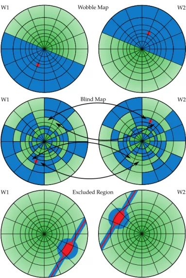
Fig. 1.Illustration of the different methods for the construction of a background camera exposure model from Wobble observations (here one Wobble pair). The source position and extension is shown as red point, ellipse or stripe. The blue shading marks bins excluded from the background map reconstruction.

telescope pointings are weighted with the time spent in the cor- responding direction and binned into an Az

/

Zd histogram, the so-called pointing history, with the Zenith distance (Zd) binned in terms of cos(Zd).

To estimate the IRFs of the MAGIC telescopes (also needed in the aperture photometry approach), the MAGIC collabora- tion generates MC simulated event sets, in which the simulated events are distributed across the entire sky. Out of this event pop- ulation, the events located around the centre of a filled pointing history bin are sampled to generate the IRFs. The size of the ac- ceptance box around the pointing bin centres can be chosen by the user and by default is the same as the bin size of the pointing history. The method for the background map generation deviates as it requires sampling from measured events, as explained in section 2.3.

2.3. Background map

For weak or extended sources, data collected with IACTs is strongly dominated by an irreducible background (Maier &

Knapp 2007; Sobczy´nska 2009, 2015; Sitarek et al. 2018) that

cannot be separated as mentioned in section 1. Therefore, the

distribution of background events in the observed sky-patch must be known with high accuracy to keep systematic uncer- tainties low. Such background counts are caused by the fraction of hadronic CRs surviving the event selection cuts and electron induced showers, which like

γ-ray showers are purely electro-

magnetic.

Their distribution in the observed sky region can be expected to resemble the camera response to an isotropic flux of

γ-ray

events. For long exposures, however, the background skymap de- viates from the simulated

γ-ray exposure. This may result from

discrepancies between data and simulations such as dead pix- els, stars in the FoV, imperfect flat-fielding of the camera, or a class of hadronic CRs surviving the cuts, but still having an ac- ceptance distribution di

ff

erent to the one of

γ-rays. Hence, one

needs to compute the background from measurements.

This background measurement must be preformed under the same observational conditions and follow the same pointing his- tory as the ON data. Such so-called ON-OFF observations are an established mode of observation for IACTs, but are only rarely used due to the additional time needed for the OFF observations and lost for the ON source observations.

For sources that are point-like or have limited extension (< 1/2 FoV) the established mode of observation is the so-called wobble mode (Fomin et al. 1994), where the telescope points in an alternating way to coordinates at a fixed o

ff

set around the object. This way ON and OFF measurements can be performed simultaneously since the background can be obtained from an- other part of the camera of similar acceptance as the source posi- tion; the alternation cancels out possible inhomogeneities in the camera halves.

We have implemented three di

ff

erent methods to recon- struct a background exposure model for the whole camera from wobble mode observations. Two of these methods are re- implementations of established techniques (called Wobble and Blind Map; Moralejo et al. 2009) used in MARS to generate sky maps. The third method (Exclusion Map) is an advancement of the concept regarding generalization and flexibility. All three methods follow the same basic scheme:

1. All events passing the selection criteria along the pointing track of the telescopes are binned in horizontal coordinates and grouped by Wobble pointings.

2. A 2D histogram binned in camera coordinates is filled for each Wobble and pointing history bin.

3. For each pointing history bin the program constructs one camera exposure model out of the di

ff

erent wobble point- ings.

4. The background model in celestial coordinates is populated by random sampling from the corresponding camera expo- sure models, and applying the correct coordinate rotations and observation time weights along the pointing track.

The methods di

ff

er in the way the camera exposures for each wobble pointing are combined into a single assumed source-free background camera exposure model (step 3). The available op- tions illustrated in Fig. 1 are:

– Wobble Map:

the single camera exposures are divided into halves, such that the nominal source position (centre of the wobble setup) is contained in one half, and the normal vec- tor on the separating line is pointing away from this coor- dinate. The combined background camera exposure model is obtained by normalizing and summing up the source-free halves. This method can only be applied if the

γ-ray emis-

sion is confined inside a circle around the nominal source position with a radius corresponding to the Wobble o

ff

set.

– Blind Map:

the single camera exposures are normalised by the exposure times. From those the combined background camera exposure is obtained by using the median values in each pixel. The median automatically suppresses too large counts from possible sources. This method has the advan- tage that no prior knowledge about the distribution of

γ-ray

sources inside the FoV is needed. However, if only two wob- bles are used, the Blind Map by construction underestimates the background, though MARS routines contain a bias cor- rection to compensate for this effect. Also the presence of strong sources will inevitably lead to an upward-bias of the background model in the corresponding regions, causing a systematic flux underestimation for those objects.

– Exclusion Map:

here the analyser must specify regions con- taining known or expected sources, which can have circular or line shape. Those regions are then excluded from the com- putation of the median as described in the previous method.

Special care is required in order not to exclude too large re- gions, as this might leave no remaining options for the back- ground extraction for certain camera bins.

2.4. Point spread function

IACTs, like all imaging systems, have a finite angular resolution described by the point spread function (PSF). It is defined by the extension of an idealised point-like object, placed at infinity, in the final reconstructed image. Accordingly, the PSF can be seen as the probability function

P^{i j}_αβ

for reconstructing a detected event in the bin

αβ

instead of

i j

corresponding to its original arrival direction.

For MC simulated events the reconstructed and original arrival direction (as reconstructed by a perfect instrument) is known, so one can estimate the angular response. MC events are sampled around the track of the source in the horizontal co- ordinate system as explained in section 2.2. For each event the vector between the reconstructed and original arrival direction in camera coordinates is computed. This vector is finally rotated into the equatorial coordinate system according to section A. The sum of all events will describe the shape of a point-source ob- served along the track of the target.

Since the number of MC events is limited, the simulated shape of the PSF is noisy and the PSF is better modelled by a smooth, analytical function. For MAGIC, a 2D double Gaus- sian (Aleksi´c et al. 2016b) or a 2D King (Vela et al. 2018) func- tion were found to describe the PSF well. Because of the lower number of free parameters this analysis used the King function:

K

(r, σ, γ)

=

1

2πσ

²

1

−

1

γ

!

1

+ r²

2σ

²γ

!^−γ

,

(1)

where

σ

sets the angular scale of the resulting profile and

γ

de- termines the weight of the tails. To allow for an asymmetry of the MAGIC PSF, the distance variable

r

is defined as follows:

x_r=

(x

_αβ

cos(φ)

−y_αβ

sin(φ))

yr=

(x

αβ

sin(φ)

+yαβ

cos(φ))

r= p

x²_r +

(y

r

)

²,

(2)

where

φ

is a positional angle and is the asymmetry parame- ter, which accounts for the non-symmetry of the MAGIC sys- tem (which has only two telescopes; Aleksi´c et al. 2016b; Vela et al. 2018) as well as the influence of the Earth’s magnetic field.

The King function is fitted to the simulated point-source shape

and finally evaluated on a su

ffi

ciently large grid around the cam-

era centre.

2.5. Exposure map

The effective area of a telescope corresponds to the size of an ideal detector (with a 100% detection e

ffi

ciency) recording the same number of events as the real instrument. It can be defined as the product of the physical detector size and the detector e

ffi

- ciency

ε_Det

. For IACTs, it is usually estimated with Monte Carlo simulations, where the detection e

ffi

ciency is a ratio of the de- tected events to the simulated ones:

Aeff = N_det Nsim

×πr_sim² =ε_Det×πr_sim² ,

(3) where

Ndet

is the number of detected MC events,

Nsim

the num- ber of originally simulated events, and

rsim

is the maximal sim- ulated distance between the impact point of the shower axis and the telescope (impact parameter), playing the role of an assumed physical detector size.

The Cherenkov light density in the EAS depends on the en- ergy of the primary particle resulting in an energy dependence of the detection e

ffi

ciency – and thus the collection area. Addition- ally, the limited extension of the EAS and the size of MAGIC trigger area (smaller than the camera size – has a radius of 1.17

^◦

vs. 1.75

^◦

; Aleksi´c et al. 2016a)) lead to the drop of the camera acceptance towards its outer regions, resulting in an non-uniform camera response to

γ-ray sources at diff

erent distances from the centre of the FoV. All these e

ff

ects are reproduced in the MAGIC MC simulations.

To correctly estimate the MAGIC detection e

ffi

ciency from those MC for a specified observation, we follow the procedure outlined in section 2.2, but instead of filling the pointing his- tory just with time weights, the e

ff

ective observation time

T_eff

for each pointing bin is estimated. It is the sum of the durations of all observational runs in that pointing bin excluding possible gaps of more than 2 seconds and correcting for the instrument’s dead time.

For each pointing bin the program samples events from the MC set and transforms them into the skymap: the program com- putes the di

ff

erence between the simulated pointing direction for the telescope and the arrival direction of the event. This vec- tor is added to the equatorial coordinates of the pointing bin (see also appendix A). Each event is additionally re-weighted according to the assumed source spectrum with the weights

w(E) = F(E)/M(E), where F(E) is the source spectrum and M(E) is the energy spectrum used for the Monte Carlo gener-

ation. Due to the limited size of the MC sample, the statisti- cal noise in the obtained maps can exceed the tolerance level of

∼

5 % required for the accuracy of subsequent source anal- ysis. To overcome this noise, we fit the e

ffi

ciency model with a modified Gaussian function:

xr=

(x

i j

cos(φ)

−yi j

sin(φ))

yr =

(x

i j

sin(φ)

+yi j

cos(φ))

−

→r =

(s

1xr,s2yr

)

l²_x=

[r

−

arctan(r)]

²_x/(2σ²_x

)

l²_y=

[r

−

arctan(r)]

²_y/(2σ²_y

)

ε^Det_{i j} =A×

exp (−(l

²_x+l²_y

))

.

(4)

This parametrisation correctly reproduces the change of the MAGIC detection e

ffi

ciency throughout the FoV for a wide range of energies, encompassing those usually selected for data analysis. To perform the fit we assume that the number of simu- lated

n_{i j}

and detected

k_{i j}

events in each camera pixel (i j) follows the binomial distribution

Pi j

ki j|ni j, ε^Det_{i j}

= ni j

k_{i j}

!

ε^Det_{i j} k_{i j}

1

−ε^Det_{i j} n_{i j}−k_{i j}

.

(5)

The best-fit is obtained by minimising the log-likelihood func- tion

ln(L)

=X

i j

k_{i j}

ln

ε^Det_{i j}

+X

i j

n_{i j}−k_{i j}

ln

1

−ε^Det_{i j}

,

(6)

where we have dropped the term

P

i j

ln

_{ni j}

k_{i j}

as it does not depend on the function of interest

ε^Det_{i j}

. The minimiser used is Minuit2

³

provided by ROOT, which estimates the parameters of the mod- ified Gaussian model and their uncertainties.

The e

ffi

ciency models, obtained this way, are converted to the collection area via Eq. 3 and, by multiplication with the estimated e

ff

ective time

T_eff

, to exposure models. This proce- dure is repeated for each energy bin, selected for analysis in the SkyPrism settings.

To estimate the uncertainties of the camera e

ffi

ciency mod- els, resulting from the fit, we simulate a number (usually 100) of representations of the model parameters (A, φ,

s1,s1, σx, σy

).

The program constructs the parameter sets by drawing random numbers from a multivariate Gaussian distribution and combin- ing them with the covariance matrix from the best fits. The e

ffi

- ciency models for each of these simulations are stored and can be supplied to the spectral fitting routines of SkyPrism for prop- agating the fit uncertainties to the flux and spectral parameters estimation.

2.6. Energy dispersion

As well as the reconstructed arrival direction of an event, the reconstructed energy is affected by the detector response and the reconstruction procedure. An event, whose energy falls into a true energy bin

k, may be wrongly classified into a reconstructed

energy bin

l. This transfer of events between the energy bins can

be described by a 2D matrix

D_kl

, called the energy migration or dispersion matrix:

Cobs

E⁰_l

=X

k

D_kl E⁰|ECreal

(E

k

)

,

(7) where

Cobs

(E

_l⁰

) is the measured number of event counts and

Creal

(E

_k

) the count distribution as emitted by the source. For convenience, the migration matrix is normalised along the re- constructed energy axis

E⁰

X

l

D_kl E⁰|E=

1

,

(8)

which is equivalent to assuming that an event with true energy

E

will be with 100% probability contained in the

E⁰_l

set.

The energy matrix for a given observation is generated from MC events selected and weighted in the same way as the PSF construction. For the PSF and Exposure program, the user can switch between generating the IRFs in

E

or

E⁰

. By default, SkyPrism uses a wider energy range in true energy than that in reconstructed energy, specified by the user. This accounts for the possible spill-over of the events from energy bins outside the analysed energy range to those used in the analysis. By extend- ing the energy range in

E

down to 1/3

E_min⁰

and up to 3

×E⁰_max

, we ensure that the lowest and highest true energy bins contribute no more than 10% to the flux in the

E⁰

range. Furthermore, the number of bins in

E

is increased compared to

E⁰

to allow for an

3 https://root.cern.ch/guides/minuit2-manual

accurate flux reconstruction when changing the spectral parame- ters during the maximal likelihood fit and to account for possible sharp spectral features such as cut-o

ff

s or bumps. By default the binning in the true energy is chosen to approximately match the energy resolution of the MAGIC telescopes.

2.7. Likelihood fitting of the sky maps

The extraction of the information of the observed sources, such as the flux and the extension, is performed by a set of Python

⁴

routines, which can be accessed from a user script. This way the fit and analysis procedure can be adapted to the user’s needs and easily be extended beyond the foreseen functionality presented here.

The fitting procedure combines background, PSF, energy mi- gration matrix and exposure information obtained in the previous steps to provide the maximum likelihood estimate of the fluxes of the sources specified by the user.

Internally, IRFs (e.g exposure and PSF) are represented as 2D images for each of the energy bins where the analysis takes place; they are prepared by the tools described above and loaded at the moment of fitting. The source images are prepared dur- ing runtime based on the information, provided in the “source model”:

–

for point sources the corresponding image contains one filled skymap bin at the specified source position;

–

for extended sources the image is taken either from a prede- fined FITS

⁵

(Wells et al. 1981) file or a 2D array filled by the user inside the analysis script.

Such source maps are further interpolated to exactly match the pixel grid of the sky, background and exposure maps. In each energy bin, the best-fit estimate of the source fluxes is obtained by maximising the Poissonian likelihood of the observed number of counts given the source model and background:

C_αβ^mod=X

p

hS^p_{i j}× E_{i j}

⊗ P^{i j}_αβi

+B_αβ

(9)

L=Y

αβ

e^−Cmodαβ C_αβ^modC

obsαβ

C_αβ^obs

! (10)

C_αβ^obs

are the measured counts in each pixel of the sky map,

S_{i j}^p

the model source (p denotes the source number in the model),

E_{i j}

the exposure maps, and

B_αβ

the background maps, while

P^{i j}_αβ

is the PSF model, mapping an (i,

j) pixel to (α, β). Com-

putationally the program minimises the negative log-likelihood

−

ln(L) using

iminuit⁶

. Following the Wilks theorem (Wilks 1938), the uncertainties on the obtained fluxes are computed as deviations of the log-likelihood from its best value by

∆

log

L= χ²₁

(α) (since there is only one parameter of interest – flux), where

α

is a desired confidence quantile. Additionally, we have also implemented a Markov-Chain-Monte-Carlo (MCMC) sam- pling procedure, based on the

emcee⁷

(Foreman-Mackey et al.

2013) library, which allows a more accurate computation of non- symmetric error bars in case of strong correlations between the fit parameters (e.g. if overlapping extended sources are specified in the model).

4 https://www.python.org/

5 https://fits.gsfc.nasa.gov/fits_documentation.html

6 http://iminuit.readthedocs.io/en/latest/

7 http://dfm.io/emcee/current/

In addition to the fit of individual source fluxes, the imple- mented procedure also allows for the source positions to be fit- ted. For this the supplied source models

S_{i j}^p

are shifted with respect to the originally specified position; the amounts of the shifts are optimised with the rest of the parameters during the fit. A more sophisticated source position

/

extension scans can be easily implemented in the user analysis script – altering the source model and repeating the fit of the already loaded data.

2.8. Likelihood fitting considering the energy migration

In addition to fitting of the individual data bins in reconstructed energy, the SkyPrism Python library can also fit in the true en- ergy space via a forward folding procedure. In this case the as- sumed source spectrum is integrated in all true energy bins

E_k

, multiplied with the exposure, and convolved with the PSF cor- responding to them. Through a multiplication with the energy migration matrix, the predicted counts of each model compo- nent in the reconstructed energy bin

E⁰_l

are obtained. The sum of all components together with the background image (which is always constructed as a function of the estimated energy

E⁰

, as it comes from data directly) leads to the model counts in

E⁰

:

C^mod_αβ

(E

_l⁰

)

=X

k p

D_klh

S^p_{i j}

(E

k

)

× E_{i j}

(E

k

)

⊗ P^{i j}_αβ

(E

k

)

i

+B_αβ

(E

⁰_l

)

.

(11) The likelihood function in this case is defined as a product of all

E⁰

bins in Eq. 10, which is then optimised with respect to the model parameters via the same routines as described in section 2.7.

As opposed to the fits in terms of the estimated energy (Eq. 9), the reconstruction of the separate flux points in the true energy space is not a well-defined procedure. It requires assump- tions of the source spectral shape between the points (or, equiv- alently, inside the energy bins, defined in the true energy space).

In SkyPrism such differential flux points are interpreted as the nodes of the source spectral model, which uses a linear inter- polation of the inter-node energies in the log

E −

log

dN/dE

space. This is equivalent to a broken power law with multiple energy break. If the user chooses such a fit during the run time, SkyPrism will use such spectral models for all the sources in Eq. 11 and perform the fit as usual. In this case the energies of the desired data points (nodes) can be chosen freely.

The output of this fit can be used e.g. to assess the validity of the chosen source spectral model. We, however, would like to underline, that the resulting data points (along with their un- certainties) may be strongly correlated and cannot be used as independent measurements in third-party analyses.

3. Validation on MAGIC data

To ensure that the SkyPrism tools and routines work as expected, we have performed a series of tests for every part of the package.

For the tests, we employ the standard MAGIC Monte-Carlo sim- ulations, that cover all the low-level data reductions and compare the tools outputs with the (a) real data and (b) results of the stan- dard MAGIC data analysis with MARS.

3.1. Background map

As the normalization of the background can be refined during

the maximum likelihood fit, the background model, described in

details in section 2.3, only needs to match the real background

distribution in shape. In order to estimate a possible mismatch, we have performed

–

a comparison of the model with the isotropic background, obtained through a simplified simulation of a typical MAGIC observation;

–

a comparison of the obtained model with the sky map for an observation of an empty region of sky.

The simulation has the advantage of eliminating possible small variations of the real instrument performance, providing the con- sistency check of the procedure itself, whereas the comparison with real data demonstrates the overall performance with all the imperfections included.

For the comparison with the simulated events, we took the MAGIC track on the sky during one of the low zenith angle ob- servations (Zd

<

35

^◦

) and simulated various number of events isotropically distributed over the field of view along the track.

The number of simulated events matches to what is usually recorded with the typical analysis criteria in the energy range above 100 GeV with exposure times of 3 to 30 hr. These events were supplied to the Blind map procedure of SkyPrism, with no modifications to the reconstruction settings.

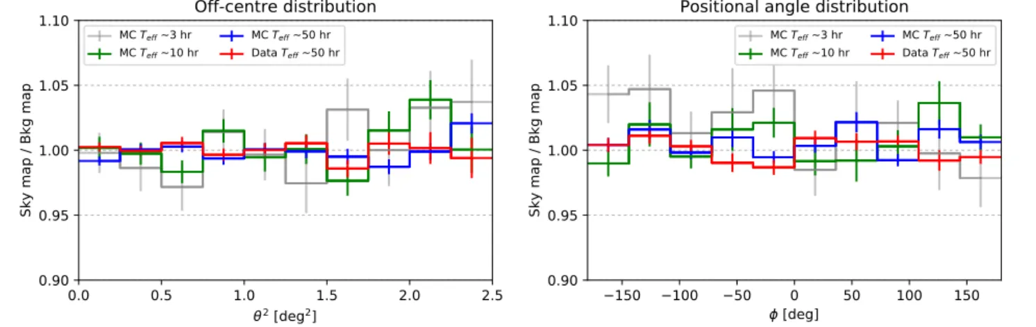
A comparison of the simulated event distribution with the re- constructed background, obtained in this way, is given in Fig. 2.

The left panel of Fig. 2 shows the radial distribution of the sim- ulated events with respect to the reconstructed background as function of the o

ff

set from the pointing centre. As it can be seen, the performance of the reconstruction method degrades towards the edges of the field of view, where the MAGIC collection area is lower and less events are recorded. Still, spurious background variations, resulting from the SkyPrism methods, do not exceed

∼

5% even for short exposures (∼ 10 h). For longer exposures of more than 10 hours, variations are in general less than 2-3% in the 3.5 deg wide field of view. Similar conclusions can be drawn from the right panel of Fig. 2, depicting the reconstructed back- ground variations as a function of the polar angle with respect to the observation pointing centre.

Additionally, we tested the di

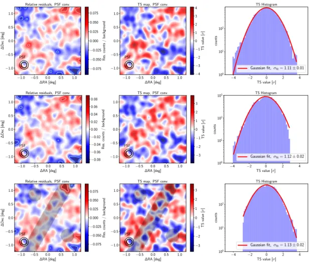
ff

erent background models available within SkyPrism by comparing them to the ON sky map of an empty sky region observed for 50 hr with four wobble pointings. For this purpose, the background model was scaled to match the ON sky map in terms of the median and subtracted from the latter. The residuals were examined in terms of relative flux (residual counts over the background) and test statistic (TS) value. The TS was constructed by sampling 500 times from the background model, using Poissonian random numbers in each pixel. We smoothed the map with a kernel of approximately the size of the PSF to obtain the TS values, roughly equivalent to putative point sources in the field of view. After smoothing, the residuals of the background-subtracted simulations very closely follow a Gaussian distribution around zero in each pixel. We thus define the TS as the local deviation in units of the Gaussian

σ.

The results of this test can be seen in Fig. 3. As one can see, all three background estimation methods show a similar perfor- mance.

The distribution of the TS values matches the normal distribution well enough to not lead to the detections of spurious sources in the image. This can be seen from the the fitted

σ_map

values, given in each TS histogram plot of Fig. 3. These values are approximately 1.1

±

0.02, indicating a slight excess on top of the statistical fluctuations alone. This excess is likely due to a small shape discrepancy between the background model and the observed empty field. Assuming that the statistical error

σstat

and systematic uncertainty

σsys

of the model are both normally

distributed, we can quantify the contribution from the systematic component as

σsys = q

σ²_map−σ²_stat

. This yields

σsys ≈

0.46 in units of standard deviation of the simulated background maps.

This latter is

≈

1.8% of the background flux, suggesting that the systematic uncertainty of the SkyPrism background maps is

∼

1% – a level comparable to the quoted systematics of the MAGIC telescopes (Aleksi´c et al. 2016b).

It should be noted, that the statistical uncertainty of the con- structed background model depends significantly on the event selection criteria. For relaxed cuts and a wide energy range, similar to the ones used here, the relative statistical back- ground uncertainty would scale with the observation time as

∼

2%

√

50 h/t

obs

.

3.2. Point spread function

As mentioned in section 2.4, the MAGIC point spread function in general is not circularly symmetric. This instrumental e

ff

ect is covered by the MAGIC MCs, but not considered in the stan- dard MAGIC analysis. Instead, the standard MAGIC spectrum extraction tool collects the signal from a circular region around the source, whose extension is usually chosen to contain a sig- nificant fraction (

&

75%) of the signal. This way the positional angle dependence of the PSF has a minor impact on the recon- structed source fluxes in most of the applications of the standard MAGIC analysis chain.

For a 2D image analysis of MAGIC data this e

ff

ect can not be neglected. For certain observational configurations it would result in noticeable residuals and, consequently, a possible bias in the fit – especially in crowded regions. To ensure that the e

ff

ect is properly reconstructed with the SkyPrism tools, we performed a 2D fit of the reconstructed PSF profiles with the King function (see section 2.4 for details), which we compared to the real data.

For this comparison we used a recent MAGIC observation of Mrk 421 at low and medium zenith angles in the energy range from 100 GeV to 10 TeV. Since the PSF calculation pro- cedure, described in section 2.4, selects only a subsample of available Monte-Carlo events (so that it matches the azimuth and zenith angle distributions of the observations), the number of MC events at the edges of the used energy range is limited.

Due to this we dropped the highest (lowest) energy bin for the low (medium) zenith range analysis in order to avoid issues re- lated to the low statistics limit.

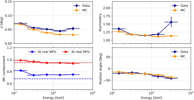
In Fig. 4 and 5 we show the comparison of the King func- tion fit results to the low and medium zenith angle data sample as well as to the corresponding MC PSF profile, computed with SkyPrism. It is evident that the Monte-Carlo estimated PSF is sharper than the real data profile – the relative event containment di

ff

erence is

∼

10%, estimated at the angular distance, where the measured event containment is 68%. At larger distances, corre- sponding to 95% containment of the real data, the Monte-Carlo data mismatch is reduced to

.

5%. This is comparable to the results obtained in Aleksi´c et al. (2016b).

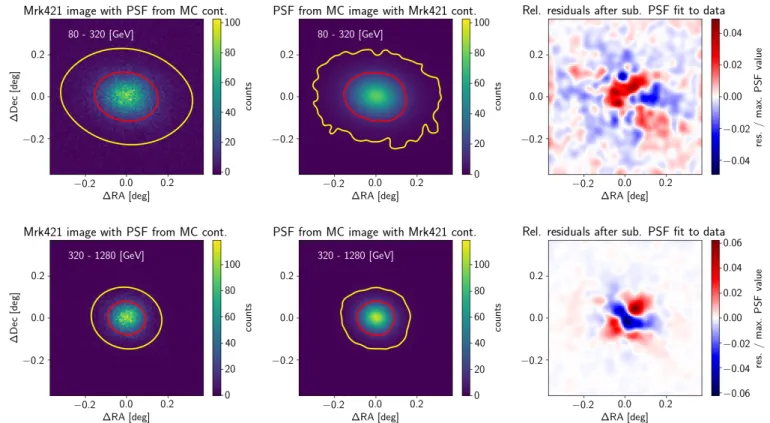
The excessive peakedness of the core of the MAGIC MC

PSF was already demonstrated earlier (Aleksi´c et al. 2016b). In

practice an additional systematic random component of

∼

0.02

^◦

should be added in order to compensate MC to data di

ff

er-

ence (Aleksi´c et al. 2016b). Indeed, the addition of 0.02

^◦

smear-

ing to the MC PSF results in

.

5% residuals in the 2D data-to-

model comparison plots, shown in Fig. 6, throughout the entire

PSF extension.

0.0 0.5 1.0 1.5 2.0 2.5

2

[deg

²

] 0.90

0.95 1.00 1.05 1.10

Sky map / Bkg map

Off-centre distribution

MC Teff ~3 hr

MC Teff ~10 hr MC Teff ~50 hr Data Teff ~50 hr

150 100 50 0 50 100 150

[deg]

0.90 0.95 1.00 1.05 1.10

Sky map / Bkg map

Positional angle distribution

MC Teff ~3 hr

MC Teff ~10 hr MC Teff ~50 hr Data Teff ~50 hr

Fig. 2.Comparison of a simulated sky map with no source and a background profile, reconstructed from it with SkyPrism. Also shown is a similar profile, obtained from the real empty field data with the BlindMap method of the SkyPrism analysis.Left: Off-centre distribution.Right: Positional angle distribution; zero point is arbitrarily set to a horizontal direction.

Certain small di

ff

erences between the MC estimated PSF and real data, apparent in the right panels in Figs. 4 and 5 play a sec- ond order role when the MAGIC mispointing is considered. We have checked that the largest deviation in asymmetry for 0

^◦−35^◦

zenith angle (Fig. 4) range comes from the low number of counts in the source image in the energy bin 2.1 - 4.6 TeV. At larger zenith angles in Fig. 5, the di

ff

erence in MC and real PSF asym- metries in 215 - 464 GeV bin appears significant due to the insuf- ficient number of MC events surviving the selection cuts, which results in a significant underestimation of the corresponding er- ror bars.

Overall, the comparison above demonstrates a reasonable agreement between the Monte-Carlo PSF model, computed with the presented software, and real data.

3.3. Exposure map

As described in section 2.5, the exposure and e

ff

ective area pri- marily depends on the energy. For a point source our programs should reproduce the same energy dependence of e

ff

ective area as the standard analysis. As the analysis approach is di

ff

erent, we need to reproduce the aperture photometry approach for esti- mating the e

ff

ective area: we cut a circular aperture out of the ef- fective area map and average the effective area inside weighting each bin according to the PSF distribution. This way we obtain the e

ff

ective area curve for a point source inside a certain area.

The size and the data set used are the same as in Aleksi´c et al.

(2016b).

Figure 7 shows the comparison of the SkyPrism result with those from Aleksi´c et al. (2016b) for two di

ff

erent Zenith dis- tance ranges, low (Zd

<

30

^◦

) and medium (30

^◦<

Zd

<

45

^◦

). One can see that with higher energy the e

ff

ective area increases as showers more distant from the telescopes can be recorded. The curves obtained with both methods agree for all energies within 20%. The discrepancy may well result from the difference in the approaches as they can just be made compatible to a certain extent. Furthermore, the SkyPrism analysis uses Monte-Carlo events distributed over the whole camera, whereas the analysis from Aleksi´c et al. (2016b) uses simulation of a point source at an o

ff

set of 0.4

^◦

.

As our tools should further compute the e

ff

ective area cor- rectly across the entire FoV, we validated the estimated o

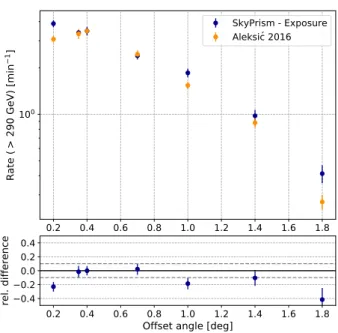
ff

-axis performance. Aleksi´c et al. (2016b) measured the rate from the

Crab Nebula depending on the o

ff

set pointing distance from the source to determine the o

ff

-axis acceptance. The measured rate and the e

ff

ective area o

ff

-axis dependence di

ff

er only by a sin- gle factor, given by the integral spectrum of the source above a considered threshold energy. Since this factor is a constant (for steady sources such as the Crab Nebula), the measured rate and the e

ff

ective area have the same dependency on the o

ff

-axis an- gle.

We computed the e

ff

ective area for the o

ff

-axis data sets of the rate measurement. The e

ff

ective area was extracted for each o

ff

-axis angle separately in the same way as for the en- ergy

/

e

ff

ective area comparison. We multiplied the e

ff

ective area at each o

ff

set with the integral spectrum extracted with SkyPrism at 0.4

^◦

o

ff

set to obtain the expected rate. Fig. 8 shows that the ef- fective area estimates agree with the measurements in nearly all bins within the errorbars, and the relative difference is less than 20% except for 1.8 deg o

ff

set. The MAGIC MC simulation in- clude events up to 1.5 deg o

ff

set, hence at 1.8 deg we need to rely on the extrapolation from the fit to the exposure model and thereby the SkyPrism estimation is approximately correct.

Considering known di

ff

erences between SkyPrism and the standard MARS analysis, as well as the limited FoV in the MC simulations, the estimations and measurements agree between both approaches. Hence, the SkyPrism package is able to cor- rectly compute the effective area across the MAGIC FoV.

3.4. Source flux estimation through the likelihood fit

A final test to the overall performance of the SkyPrism package – and its image fitting routines in particular – is to reproduce the spectrum of a well-measured source. It is natural to use the Crab Nebula, given that it is among the brightest steady sources in the TeV energy band and is widely used as a calibration object in the IACT community. Here we used the MAGIC Crab Nebula observations at low (0

^◦−

30

^◦

) zenith angle.

The fit setup for this test includes the PSF,

γ-ray exposure

and background model, estimated with SkyPrism, and employs the MAGIC data in the energy range from 60 GeV to 10 TeV.

The fitted model includes the point source at the Crab Nebula position and an isotropic background.

The resulting spectrum, presented in Fig. 9, does not show

any significant deviations from the reference spectrum, derived

by MAGIC (Aleksi´c et al. 2016b). Though the accuracy of

−1.0 −0.5 0.0 0.5 1.0

∆RA [deg]

−1.0

−0.5 0.0 0.5 1.0

∆Dec[deg]

Relative residuals, PSF conv.

PSF

−0.075

−0.050

−0.025 0.000 0.025 0.050 0.075

Res.counts/background

−1.0 −0.5 0.0 0.5 1.0

∆RA [deg]

−1.0

−0.5 0.0 0.5 1.0

TS map, PSF conv.

PSF

−4

−3

−2

−1 0 1 2 3 4

TSvalue[σ]

−4 −2 0 2 4

TS value [σ]

10⁰ 10¹ 10²

counts

TS Histogram

Gaussian fit,σfit= 1.11±0.01

−1.0 −0.5 0.0 0.5 1.0

∆RA [deg]

−1.0

−0.5 0.0 0.5 1.0

∆Dec[deg]

Relative residuals, PSF conv.

PSF

−0.08

−0.06

−0.04

−0.02 0.00 0.02 0.04 0.06 0.08

Res.counts/background

−1.0 −0.5 0.0 0.5 1.0

∆RA [deg]

−1.0

−0.5 0.0 0.5 1.0

TS map, PSF conv.

PSF

−3

−2

−1 0 1 2 3

TSvalue[σ]

−4 −2 0 2 4

TS value [σ]

10⁰ 10¹ 10² 10³

counts

TS Histogram

Gaussian fit,σfit= 1.12±0.02

−1.0 −0.5 0.0 0.5 1.0

∆RA [deg]

−1.0

−0.5 0.0 0.5 1.0

∆Dec[deg]

Relative residuals, PSF conv.

PSF

−0.075

−0.050

−0.025 0.000 0.025 0.050 0.075

Res.counts/background

−1.0 −0.5 0.0 0.5 1.0

∆RA [deg]

−1.0

−0.5 0.0 0.5 1.0

TS map, PSF conv.

PSF

−3

−2

−1 0 1 2 3

TSvalue[σ]

−4 −2 0 2 4

TS value [σ]

10⁰ 10¹ 10²

counts

TS Histogram

Gaussian fit,σfit= 1.13±0.02

Fig. 3.Background methods tested with an empty sky region at Zd<35^◦. Top to bottom: Wobble map, Blind map, Excluded region map. For the

“Excluded region map”, the ignored regions (a stripe and two circles) are shaded. The PSF after convolution with a smoothing kernel is depicted in terms of 39% and 68% containment contours.Left:ratio of the residuals (skymap-reconstructed background) to the skymap. The blue and red contours indicate±5% relative flux boundary.Centre:the test statistic maps computed for the residual counts in the left panels.Right:the distribution of the test statistic values (blue histogram) compared to the expected normal distribution (red curve). See Sect. 2.3 and 3.1 for details.

the o

ff

-axis SkyPrism performance estimate was demonstrated in section 3.3, we also performed additional analysis of the larger o

ff

-set observations of the Crab Nebula at 0.2

^◦

, 0.7

^◦

, 1.0

^◦

, and 1.4

^◦

(compared to the standard MAGIC 0.4

^◦

). These tests, presented in Appendix B, show the same level of agreement between the standard MAGIC analysis and SkyPrism results, though the amount of data is not su

ffi

cient to obtain statistical uncertainties of

.

10% over the entire energy range.

Overall, this reassures the validity of SkyPrism calculations.

4. Summary

We have presented a new IACT data analysis package SkyPrism, optimised for MAGIC data. The package includes several rou- tines that estimate the telescope response (as a function of the field of view and photon energy) from on Monte-Carlo simula- tions. The estimated response is computed individually for each observation, based on the telescope pointing distribution during the corresponding data taking to ensure it describes the telescope performance accurately.

We have performed extensive tests of the key ingredients of a data analysis: the PSF and

γ-ray exposure, background model

and fitting procedure. Altogether we demonstrate an agreement with the standard MAGIC analysis package, MARS (Zanin et al.

2013), at the level

.

10% in terms of the reconstructed source

flux. The accuracy of the SkyPrism analysis does not degrade with the o

ff

-set from the telescope camera centre, which enables a proper reconstruction of extended sources fluxes over the entire FoV.

With SkyPrism for the first time it is possible to analyse MAGIC data of extended sources of arbitrary morphology. It also can cope with multiple, overlapping point sources in the in- strument’s field of view, as well as combining several data set covering large sky regions in an convenient way. Though the structure of SkyPrism is di

ff

erent from CTools (Knödlseder et al.

2016) and Gammapy (Deil et al. 2017), its parts can be further optimised for the data analysis of di

ff

erent IACTs, such as the next-generation CTA.

Within the MAGIC collaboration SkyPrism will be dis-

tributed together with the future standard software releases; be-

ing open-source, it is also available from the authors upon re-

quest.

0.00 0.05 0.10 0.15

[d eg ]

Data MC

10

²

10

³

10

⁴

Energy [GeV]

0.6 0.8 1.0 1.2

MC containment

At real 68% At real 95%

1.00 1.25 1.50 1.75 2.00

Asymmetry

Data MC

10

²

10

³

10

⁴

Energy [GeV]

50 0 50

Position angle [deg]

Data MC

Fig. 4.Comparison of the MC PSF to the real data in the 0^◦−35^◦ zenith angle range, performed in terms of the King function fit.Top left:σ parameter of the King function, which defines the spacial scale.Top right: asymmetry of the fitted profile.Bottom left: Monte-Carlo events containment, computed at the radial distance corresponding to the 68% (95%) data containment radius.Bottom right: positional angleφof the non-symmetric PSF extension.

0.00 0.05 0.10 0.15

[d eg ]

Data MC

10

²

10

³

10

⁴

Energy [GeV]

0.6 0.8 1.0 1.2

MC containment

At real 68% At real 95%

1.00 1.25 1.50 1.75 2.00

Asymmetry

Data MC

10

²

10

³

10

⁴

Energy [GeV]

50 0 50

Position angle [deg]

Data MC

Fig. 5.Comparison of the MC PSF to the real data in the 35^◦−50^◦zenith angle range, performed in terms of the King function fit. Panels are the same as in Fig. 4

Fig. 6.PSF model validation on Mrk421 data taken at zenith angles<30^◦in two energy ranges: 80 GeV to 320 GeV (top group) and 320 GeV to 1280 GeV) (bottom group). The first column shows the source images with the 68% and 95% level contours of the corresponding PSF model;

second column gives PSF model with the 68% and 95% containment contours of the sky map. The right column shows the residuals after subtracting the normalized PSF model from the sky image.

10² 10³ 10⁴ Energy [GeV]

10⁴ 10⁵

Eff.Area[m2]

Aleksi´c 2016 - low Zd Aleksi´c 2016 - med Zd SkyPrism - low Zd SkyPrism - med Zd

Fig. 7.Effective area vs. energy as estimated with the SkyPrism package compared to the standard MAGIC analysis from Aleksi´c et al. (2016b).

0.2 0.4 0.6 0.8 1.0 1.2 1.4 1.6 1.8

10

⁰

Ra te (> 29 0 Ge V) [m in

1

]

SkyPrism - Exposure Aleksic 2016

0.2 0.4 0.6 0.8 1.0 1.2 1.4 1.6 1.8

Offset angle [deg]

0.4 0.2 0.0 0.2 0.4

rel. difference

Fig. 8.Crab Nebula count rate as a function of the off-axis angle. Or- ange points correspond to Aleksi´c et al. (2016b), the blue denote the estimates from the SkyPrism exposure model, obtained for the same data and selection cuts. The bottom panel shows the relative difference between both data sets at each offset angle.

10¹¹ 10¹² 10¹³

Energy [eV]

10¹ 10²

E2dN/dE[eVcm−2s−2]

0.4^◦wobble dist.

SkyPrism - forward folding Aleksi´c et al. (2016) SkyPrism in Eest

10¹¹ 10¹² 10¹³

Energy [eV]

−0.4

−0.2 0.0 0.2 0.4

∆F/F

Fig. 9.SED of the Crab Nebula obtained by processing the data set used by Aleksi´c et al. (2016b) with the full SkyPrism tool chain. The spectral fit is obtained via the forward folding procedure, whereas the data points are the results of the individual fits in eachEest bin. The dark blue error bars of the data points are the statistical error and the light blue ones indicate the uncertainties from the exposure model. The obtained results are also compared to the Crab Nebula SED from the same publication in terms of the relative flux difference (∆F/F.)

Appendix A: Transformation from Azimuthal to Equatorial Coordinates

While the instrument response depends on the horizontal coordi- nate system, the emission of astrophysical sources and the back- ground depend on the skyfield, which is preferably defined in a Celestial coordinate system such as the Equatorial coordinate system.

For usual observations the horizontal and equatorial coordi- nates for the centre of the MAGIC camera are recorded, so the time dependence of the transformation can be factored out. The sampled IRFs can be transformed from horizontal coordinates to equatorial ones via a rotation by an angle

β, which can be com-

puted using the so called navigational triangle: it is formed by the pointing position, the celestial north pole, and the Zenith. As the Azimuth

γ, the latitude of the observatoryφ

(b

=

90

^◦−φ),

and the Zenith distance of the pointing

a

are known the rotation angle can be calculated via:

c=

arccos (cos (a) cos (b)

+

sin (a) cos (b) cos (γ)) (A.1)

β⁰=

arcsin (sin (b) sin (γ)

/

sin (c)) (A.2)

β=

(β⁰

if cos (a) cos (c)

≤

cos (b)

π−β⁰

else (A.3)

with c being the distance between the pointing and the celestial north pole.

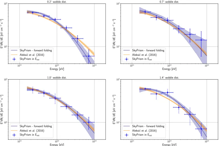
Appendix B: Source spectra estimation at different camera off-set angles

As a demonstration of the performance of the SkyPrism tools for non-standard source positions with respect to the camera center, here we also show additional SEDs from larger o

ff

-set obser- vations of the Crab Nebula, namely at at 0.2

^◦

, 0.7

^◦

, 1.0

^◦

, and 1.4

^◦

(MAGIC standard o

ff

-set is 0.4

^◦

). Similarly to the analy- sis, presented in Sect. 3.4, we used the PSF,

γ-ray exposure and

background models, constructed with SkyPrism – for each of the observations individually. The fitted source model again in- cluded just the Crab Nebula point source with the addition of the isotropic background. The obtained spectra are shown in Fig. B.1 and demonstrate a reasonable agreement between SkyPrism and standard MAGIC analysis. The data sets are comparably small, which increases statistical uncertainties.

Acknowledgements. The authors would like to thank the MAGIC Collaboration for support and providing the data and the MARS software. Particularly, we would like to thank Julian Sitarek for providing us the results of the MAGIC per- formance paper and valuable discussion throughout the preparation of this work.

The work of Ievgen Vovk is supported by the Swiss National Science Foundation grant P2GEP2_151815.

References

Acharya, B. S., Actis, M., Aghajani, T., et al. 2013, Astroparticle Physics, 43, 3 Albert, J., Aliu, E., Anderhub, H., et al. 2008, Nuclear Instruments and Methods

in Physics Research A, 588, 424

Aleksi´c, J., Ansoldi, S., Antonelli, L. A., et al. 2016a, Astroparticle Physics, 72, 61

Aleksi´c, J., Ansoldi, S., Antonelli, L. A., et al. 2016b, Astroparticle Physics, 72, 76

Antcheva, I., Ballintijn, M., Bellenot, B., et al. 2009, Computer Physics Com- munications, 180, 2499

Baixeras, C. 2003, Nuclear Physics B Proceedings Supplements, 114, 247 Berge, D., Funk, S., & Hinton, J. 2007, Astronomy and Astrophysics, 466, 1219 Breiman, L. 2001, Machine learning, 45, 5

Deil, C., Zanin, R., Lefaucheur, J., et al. 2017, ArXiv e-prints [arXiv:1709.01751]

Fomin, V. P., Stepanian, A. A., Lamb, R. C., et al. 1994, Astroparticle Physics, 2, 137

Foreman-Mackey, D., Hogg, D. W., Lang, D., & Goodman, J. 2013, PASP, 125, 306

Knödlseder, J., Mayer, M., Deil, C., et al. 2016, A&A, 593, A1 Maier, G. & Knapp, J. 2007, Astroparticle Physics, 28, 72

Mattox, J. R., Bertsch, D. L., Chiang, J., et al. 1996, The Astrophysical Journal, 461, 396

Moralejo, A., Gaug, M., Carmona, E., et al. 2009, arXiv:0907.0943 [astro-ph], arXiv: 0907.0943

Sitarek, J., Sobczy´nska, D., Szanecki, M., et al. 2018, Astroparticle Physics, 97, 1

Sobczy´nska, D. 2009, Journal of Physics G Nuclear Physics, 36, 125201 Sobczy´nska, D. 2015, Journal of Physics G Nuclear Physics, 42, 095201 Vela, P. D., Stamerra, A., Neronov, A., et al. 2018, Astroparticle Physics, 98, 1 Wells, D. C., Greisen, E. W., & Harten, R. H. 1981, A&AS, 44, 363

Wilks, S. S. 1938, Ann. Math. Statist., 9, 60

Zanin, R., Carmona, E., Sitarek, J., Colin, P., & Frantzen, K. 2013, in Proc. of the 33st International Cosmic Ray Conference, Rio de Janeiro, Brasil

10¹¹ 10¹² 10¹³ Energy [eV]

10¹ 10²

E2dN/dE[eVcm−2s−2]

0.2^◦wobble dist.

SkyPrism - forward folding Aleksi´c et al. (2016) SkyPrism in Eest

10¹¹ 10¹² 10¹³

Energy [eV]

10¹ 10²

E2dN/dE[eVcm−2s−2]

0.7^◦wobble dist.

SkyPrism - forward folding Aleksi´c et al. (2016) SkyPrism in Eest

10¹¹ 10¹² 10¹³

Energy [eV]

10¹ 10²

E2dN/dE[eVcm−2s−2]

1.0^◦wobble dist.

SkyPrism - forward folding Aleksi´c et al. (2016) SkyPrism in Eest

10¹¹ 10¹² 10¹³

Energy [eV]

10¹ 10²

E2dN/dE[eVcm−2s−2]

1.4^◦wobble dist.

SkyPrism - forward folding Aleksi´c et al. (2016) SkyPrism in Eest

Fig. B.1.SED of the Crab Nebula obtained by processing data with non-standard wobble offsets that has also been used by Aleksi´c et al. (2016b).

The solid error bars indicate statistical errors while the lighter coloured, wider error bars were obtained by also propagating the uncertainties from the constructed exposure model. Due to the short observation times of data sets the uncertainties of the fitted exposure map can be larger than the statistical error of the data points.