Roland Haertel ∗ †

Roland Haertel ^{∗ †}

Max-Planck-Institut für Physik, Munich, Germany E-mail: haertel@mppmu.mpg.de

The ATLAS experiment at the LHC is currently under construction at CERN and will start oper- ation in summer 2008. The Inner Detector of ATLAS is designed to measure the momentum of charged particles and to reconstruct primary and secondary vertices. It consists of a silicon pixel detector, a silicon strip detector and a straw tube detector.

For optimal performance of the Inner Detector the position of all active detector elements must be known with a precision of a few microns. The ultimate precision will be reached with a track- based alignment algorithm.

The different alignment methods currently investigated for the ATLAS Inner Detector are pre- sented, as well as the various computational aspects regarding track-based alignment. Results from simulation studies as well as results from testbeam and cosmic ray detector setups are shown and discussed.

XI International Workshop on Advanced Computing and Analysis Techniques in Physics Research April 23-27 2007

Amsterdam, the Netherlands

∗

Speaker.

†

on behalf of the ATLAS Inner Detector Alignment Group

PoS(ACAT)049

1. Introduction

Currently the LHC is built and commissioned in a ring tunnel at CERN, Geneva. The LHC is designed to accelerate two counter-rotating proton beams to 7 TeV and to collide those beams at interaction points around the ring. At one of these interaction points the ATLAS detector is located and is currently being readied for first collisions.

The ATLAS detector is designed to detect a vast array of signatures of various physics pro- cesses and excellent calibration and alignment of all detector components is paramount to achieve good performance and to fulfill the desired physics programme.

1.1 Inner Detector

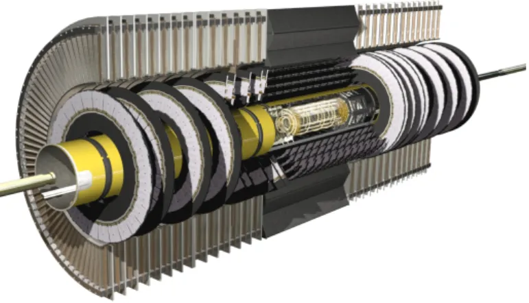
The Inner Detector of ATLAS (see figure 1) is located in a 2 Tesla solenoidal magnetic field and consists of 3 subdetectors: a silicon pixel detector (Pixel), a silicon strip detector (SCT) and a drift tube detector (TRT).

Figure 1: ATLAS Inner Detector

The Pixel detector consists of 3 cylindrical concentric barrel layers around the interaction point and 3 endcap discs on each side of the interaction point. In total 1744 identical pixel modules are mounted on the barrel layers and endcap disks. The readout pixels on a module have a pitch of 50 µ m × 400 µ m and provide a single hit resolution of 14 µ m × 115 µ m.

The SCT detector is similar in design to the pixel detector as it has a barrel and endcap layout as well. The SCT barrel consists of 4 concentric layers and the two endcap parts of 9 disks each. In total 4088 SCT modules are mounted on the barrel layers and endcap disks. SCT modules consist of two silicon strip sensors glued together back-to-back with a small stereo angle of 40 mrad. The individual readout strips are 2×6 cm long (wirebonded together) and have a pitch of 80 µ m. Barrel SCT modules have parallel readout strips whereas the readout strips of endcap modules fan out.

Each SCT readout side provides 23 µ m positioning resolution perpendicular to the strip direction.

Due to the stereo angle between the readout sides the two-sided detector resolution along the strip direction is 580 µ m.

The TRT detector is divided into barrel and endcap part as well. The barrel consists of 3 rings

of 32 modules each. Each of the two endcaps consist of 20 wheels with 8 layers each. In total there

PoS(ACAT)049

are 96 TRT barrel modules and 320 TRT endcap layers. There are about 300k individual straw tubes that have a diameter of 4 mm and will provide a resolution of 130 µ m radially to the readout wire.

1.2 Alignment

To make optimal use of the resolution of the three Inner Detector subdetectors their alignment, i.e. the position and orientation of all active detector components needs to be known. After mount- ing, installation and optical survey the alignment precision for the various subdetectors and barrel and endcap sections is different, but of the order of 100 µ m. The requirement to not degrade track parameter resolution by more than 20% is an alignment accuracy of < 10 µ m along the precision coordinate (cf. [1]).

For the purpose of alignment of the ATLAS Inner Detector each individual detector module is treated as a rigid body with only 6 degrees of freedom (3 translational and 3 rotational). At a certain level of abstraction the various support structures like endcap disks and barrel layers or a whole subdetector can be seen as rigid bodies without internal degrees of freedom themselves. Thus the alignment of the ATLAS Inner Detector is organized in hierarchical levels, namely level 1, 2 and 3 alignment.

Level 1 alignment only deals with subdetectors, endcaps and barrels and only 42 degrees of freedom, i.e. 42 alignment parameters need to be determined. At level 2, for the Pixel and SCT individual endcap disks and barrel layers are aligned and for the TRT individual barrel modules and endcap wheels. So a total of 930 alignment parameters needs to be determined. Finally, level 3 alignment tries to infer alignment constants for each module, so about 35k alignment parameters for Pixel and SCT need to be determined. For TRT at level 3 the alignment parameters of 300k straw tubes are needed.

2. Track-based Alignment

The only way to improve alignment accuracy from the approximately 100 µ m after installation to the required 10 µm or better, is with track-based alignment. Track-based alignment relies on the reconstruced trajectories of charged particles (tracks) as a way to improve the knowledge about detector positions and thus to infere alignment parameters.

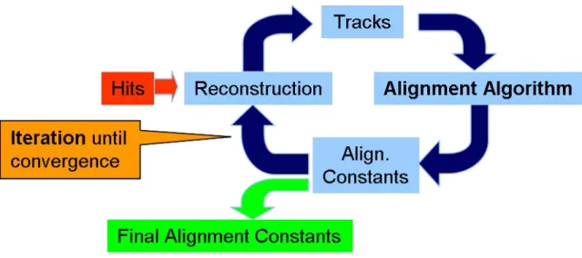
All trackbased alignment approaches for the ATLAS Inner Detector rely on residuals, where a residual is defined as the distance between a track and an associated hit. Three distinct track- based alignment algorithms have been developed for the ATLAS Inner Detector, namely the Global χ ² [2], the Local χ ² [3, 4] and the Robust [5] alignment algorithm.

All three algorithms adhere to the same general schema, outlined in figure 2. Hits in the

detector are fed into the ATLAS reconstruction software and tracks are reconstructed from this. The

resulting tracks are input to an alignment algorithm and alignment parameters are calculated. The

alignment parameters, together with the original hits are then input to a new round of reconstruction

and the improved tracks are again used in the alignment algorithm to calculate improved alignment

parameters. This procedure is iterated until it converges and the final alignment parameters pass

validation.

PoS(ACAT)049

Figure 2: Schematic diagram of the ATLAS Inner Detector reconstruction-alignment-cycle

The Global χ ² alignment algorithm does one huge linear least squares minimization (χ ² - minimization, hence the name) to fit all alignment degrees of freedom at once and thus takes all inter-module correlations into account. For level 3 alignment of the Pixel and SCT detectors this requires handling and solving of 35k×35k matrices.

The Local χ ² alignment algorithm has a similar working principle but attempts a χ ² -fit of the alignment parameters for each module individually. Thus only 6×6 matrices need to be handled, but more iterations are required to take inter-module correlations into account.

The Robust alignment algorithm works locally, i.e. on individual modules as well and uses residuals and overlap residuals to infere 2-3 alignment degrees of freedom per module. It is not a minimization procedure and requires iterations.

2.1 Global χ ² Alignment

The Global χ ² alignment algorithm is based on the following χ ² -Ansatz:

χ ² ( ~ a,~ π 1 , . . . ,~ π t ) =

∑ t i ∈ tracks

~ r i T (~ a,~ π i ) ·V _i ⁻¹ ·~ r i (~ a,~ π i ) (2.1) where~ r _i =~ r _i ( ~ a,~ π _i ) is the vector of residuals measured for track i. ~ r _i (~ a,~ π _i ) is a function of alignment parameters ~ a and of the track parameters ~ π _i . ~ a is the vector of all alignment parameters of all modules that have hits associated to at least one of the tracks. V i is the covariance matrix of the residual measurements of track i.

Linearising the χ ² -function using a Taylor expansion yields:

d χ ² ( ~ a)

d~ a ≈ dχ ² (~ a) d~ a

~ a=~ a

+ d ² χ ² ( ~ a) d~ a ²

~ a=~ a

∆ ~ a. (2.2)

Minimizing equation 2.2 with respect to the alignment parameters ~ a and then solving for the

alignment parameter corrections ∆ ~ a yields the following generic solution:

PoS(ACAT)049

∆ ~ a = − ∑

i ∈ tracks

d~ r i (~ a) d~ a ₀

· 2V _i ⁻¹ ·

d ~ r i (~ a) d~ a ₀

T ! −1

· ∑

i ∈ tracks

d ~ r i (~ a) d~ a ₀

· 2V _i ⁻¹ ·~ r i (~ a 0 )

! (2.3) For level 3 alignment of the Pixel and SCT the matrices involved are 35k×35k.

2.2 Local χ ² Alignment

Starting from the generic Global χ ² solution (eq. 2.3) the Local χ ² solution can be obtained by applying the following approximations and assumptions:

• total derivatives are substituted with partial derivatives (this neglects inter-module correla- tions)

• the covariance matrix is assumed to be diagonal (this neglects correlated errors, e.g. from multiple coulomb scattering)

With these modifications the Local χ ² solution for the alignment parameter correction ∆~ a of module k reads:

∆ ~ a _k = − ∑

i ∈ tracks

1 σ _{i k} ²

∂ r _{i k} (~ a _k )

∂~ a _{k 0}

∂ r _{i k} (~ a _k )

∂~ a _{k 0}

T ! −1

· ∑

i ∈ tracks

1 σ _{i k} ²

∂ r _{i k} ( ~ a _k )

∂~ a _{k 0}

r _{i k} ( ~ a _{k 0} )

!

(2.4) In the Local χ ² approach the 35k×35k matrices break down to 6k 6×6 matrices.

2.3 Robust Alignment

In the Robust alignment algorithm alignment parameters are calculated from mean residuals and mean overlap residuals. Overlap residuals are defined as the difference between residuals (of the same track) from overlapping modules. The alignment parameter corrections for each module are calculated with the following formula:

a _{X /Y} =

− ∑ ³ _{j=1 (δs} ^s

j

)

∑ ³ _{j=1 (δ} ¹ _s

j

)

(2.5) where, s ₁ to s ₃ are defined as:

s 1 = residual; s 2 = ∑ overlap residual _LocX ; s 3 = ∑ overlap residual _LocY (2.6) LocX and LocY denote the two directions spanning the plane of a silicon module.

3. Alignment Performance

The ATLAS Inner Detector alignment algorithms are under constant development, optimiza-

tion and validation. The performance of the algorithms has been evaluated in testbeam runs, cosmic

runs and with simulated data.

PoS(ACAT)049

3.1 Combined Testbeam 2004

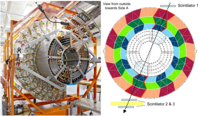
In 2004 all ATLAS subdetectors were operated in a combined testbeam (CTB) exercise. For the silicon part of the Inner Detector 6 Pixel modules and 8 SCT modules were operated in a 1.4 T magnetic field (see. figure 3). The detector was exposed to beams of different particle types and momenta. All three ATLAS Inner Detector alignment algorithms plus a forth one dedicated to CTB alignment, called Valenzia approach [6], were used to align the CTB Pixel and SCT detector.

Figure 3: Testbeam detector setup with 6 Pixel and 8 SCT modules

The CTB Pixel and SCT detector is a small but degenerate setup for track-based alignment. For example the track incident angle was always perpendicular to the module planes and only a small fraction of the sensitive area of the SCT modules was illuminated by the beam. The three alignment approaches developed different strategies to cope with this. The Robust alignment algorithm used tracks from a 100 GeV Pion run without magnetic field and derived alignment parameters for two degrees of freedom for each module. No module was fixed as anchor point. The Global χ ² alignment algorithm used the same 100 GeV Pion run without magnetic field, derived alignment parameters for four degrees of freedom per module and used two anchor points (the first Pixel module and the last SCT module). Finally, the Local χ ² alignment algorithm used no anchor points and derived alignment parameters for all six degrees of freedom per module but needed tracks from three different runs with 20 GeV and 100 GeV Pions with magnetic field and 100 GeV Pions without magnetic field. The tracks were fitted with a momentum constraint to really use the information about different particle momenta and to remove some of the degeneracies.

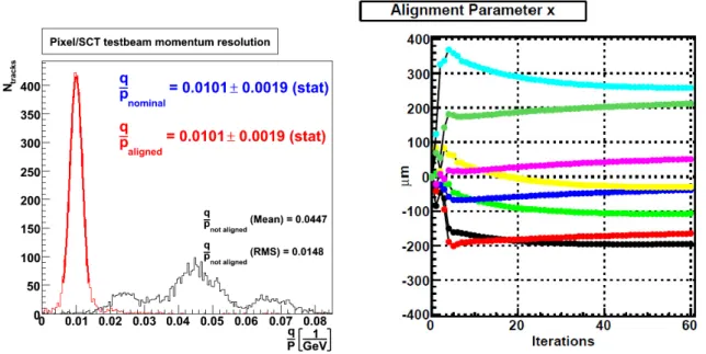
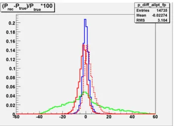
The performance of e.g. the Local χ ² alignment algorithm can be seen in figure 4. It shows the momentum resolution of the Pixel and SCT detector with (red curve) and without (black curve) the Local χ ² alignment parameters. Comparison with simulated testbeam data shows that the momen- tum resolution of a perfectly aligned detector can be recovered and that residual misalignments do not degrade detector performance. Furthermore the figure shows the convergence of one alignment parameter of all 8 SCT modules during the iterations.

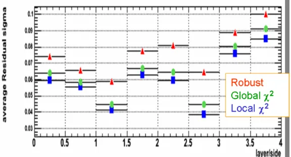
In figure 5 the momentum resolution with alignment parameters from the different algorithms

for different CTB runs is shown. The agreement of the different alignment algorithms among each

other and with simulation is remarkably good. The Robust alignment algorithms is not expected to

PoS(ACAT)049

Figure 4: Combined testbeam momentum resolution and alignment parameter x of 8 SCT modules during iterations

perform identically as it does not provide alignment parameters for all degrees of freedom that are relevant for momentum resolution.

p (GeV/c)

0 20 40 60 80 100 120 140 160 180

(p)/pσ

0 0.05 0.1 0.15 0.2 0.25 0.3 0.35 0.4 0.45 0.5

Momentum resolution electron runs with B field

p (GeV/c)

0 20 40 60 80 100 120

(p)/pσ

0 0.05 0.1 0.15 0.2 0.25 0.3 0.35 0.4 0.45 0.5

Valencia Global Robust Local Simulation

Momentum resolution pion runs with B field

Figure 5: CTB momentum resolution with different sets of alignment parameters

3.2 Cosmic runs

After integration of the SCT and TRT detector and before final installation in the ATLAS

cavern the barrel section of the SCT and TRT detector as well as one endcap section were equipped

with special triggers and operated to record data from cosmic ray particles. In both cosmic runs no

magnetic field was present and the trigger setup allowed particles with momenta as low 200 MeV /c.

PoS(ACAT)049

No method was used to harden the momentum spectrum of the tracks used for alignment and thus track fit qualitiy was affected by multiple coulomb scattering. First the alignment of the SCT and TRT barrel setup will be discussed and then the alignment of the SCT and TRT endcap setup.

3.2.1 Barrel cosmics

A schematic drawing of the SCT and TRT barrel setup is shown in figure 6. As can be seen from the drawing, 12 of the 96 TRT barrel modules and 468 of the 2112 SCT barrel modules were read out in this cosmic test setup. All three ATLAS Inner Detector alignment algorithms were used and level 3 alignment, i.e. alignment of individual modules, was attempted with 36k (Local χ ² alignment) - 200k (Robust alignment) available tracks.

Figure 6: Barrel detector setup of SCT and TRT cosmic test

In figure 7 the width (in mm) of the SCT residual distributions (averaged over the modules of one layer) is shown for the three alignment algorithms. As for the CTB alignment Global χ ² and Local χ ² alignment algorithms show very similar performance. The Robust alignment algorithm reduces residual width considerably (compared to the unaligned scenario), but does not show the same performance as the χ ² minimization algorithms, as it does not consider all degrees of freedom.

3.2.2 Endcap cosmics

For the SCT and TRT cosmic endcap setup only 20k tracks with more than 3 SCT hits were

available for alignment. This was due to the geometry of the trigger setup which only triggerd

cosmic ray particles in a very small region of solid angle and with a substatial inclination. Thus

only level 2 alignment, i.e. alignment of the SCT endcap disks was attempted. Due to the low

PoS(ACAT)049

Figure 7: Cosmic barrel test SCT residual width (in mm) with different sets of alignment parameters

number of tracks passing through 3 of the endcap disks only 6 out of 9 disks could be aligned in the end. In figure 8 the evolution of the residual width during alignment iterations is shown for the Local χ ² and Global χ ² alignment algorithm respectivley. It can be seen for the Local χ ² alignment algorithm that the residual width of disk 6 does not stabilize. This behavior is attributed to the insufficient number of tracks available. For the other disks, Global χ ² and Local χ ² again perform very similar. Iteration "-1" shows the residual width without any alignment correction, Iteration "0" shows the residual width after applying alignment corrections derived from mounting and survey data. The improvement in subsequent iterations due to track-based alignment are clearly visible.

Figure 8: Cosmic endcap test SCT residual width (in mm) with a) Local χ ² sets of alignment parameters

and b) Global χ ² set of alignment parameters

PoS(ACAT)049

3.3 Simulation

To study the performance of the ATLAS Inner Detector alignment algorithms for the full ge- ometry setup and to validate the algorithms in an controlled environment simulated data was used.

Recently 200k muon tracks were produced as part of the official ATLAS Monte Carlo production.

In this sample a misaligned geometry was included at simulation level. Various studies at alignment level 1, 2 and 3 with all three alignment algorithms and for all three Inner Detector subdetectors are currently pursued. For example in figure 9 the SCT barrel residual distributions are shown for perfectly known misalignment and for various iterations of the Global χ ² alignment algorithm.

After four iterations the residual distributions are centered at zero with a width comparable to the case of perfectly known misalignment.

Figure 9: SCT barrel residual distributions with simulated data

In figure 10 the momentum resolution of the ATLAS Inner Detector for this simulated muon sample is shown. For this study the Pixel and SCT misalignments were considered to be perfectly known and the Local χ ² alignment algorithm was used to recover the remaining TRT misalignment.

The green curve shows the momentum resolution without TRT alignment correction, the solid and the dashed red curves show the momentum resolution for positively and negatively charged muons with TRT alignment corrections determined with the Local χ ² algorithm. The blue curve shows the momentum resolution if the remaining TRT misalignment was known as well.

4. Conclusions and Outlook

In the last years three track-based alignment algorithms for the ATLAS Inner Detector were

successfully developed, tested and validated. While development, testing and validation continues,

the results of alignment studies with detector data and with simulated data are already very en-

couraging. The experience gained in aligning the combined testbeam detector and the cosmic run

detector setups shows that alignment is a vital step to ensure optimal detector performance prior to

any physics analysis.

PoS(ACAT)049

Figure 10: Momentum resolution with remaining (corrected) TRT misalignment

If anything, the alignment effort is gaining more momentum as the detector installation and commissioning is stepwise nearing completion and the startup of LHC draws nearer. Further and more exhaustive studies with simulated data are currently undertaken. Additionally there will be combined cosmic runs of the ATLAS Inner Detector together with the calorimeter and muon system in the ATLAS cavern. The detector data from these cosmic runs will again be a very challenging but also very fruitful task for the ATLAS Inner Detector alignment community.

Working on common tasks with three different algorithms helped that the different efforts within the alignment community are converging and that common tools, infrastructure and valida- tion machinery were developed. Currently, further steps are taken towards even tighter integration of the three alignment algorithms.

Finally, the ATLAS Inner Detector alignment community is looking forward to the first data from LHC collisions and to use this data to ensure optimal performance of the Inner Detector of ATLAS.

References

[1] ATLAS Collaboration. ATLAS Inner Detector, Technical Design Report Volume 1. CERN/LHCC 97-16, 1997.

[2] S. Haywood P. Bruckman, A. Hicheur. Globalχ ² approach to the alignment of the atlas silicon tracking detectors. ATL-INDET-2005-002, 2004.

[3] R. Härtel. Iterative local χ ² alignment approach for the atlas sct detector. Diploma thesis, TU München, 2005. MPP-2005-174.

[4] T. Göttfert. Iterative local χ ² alignment algorithm for the atlas pixel detector. Diploma thesis, Universität Würzburg, 2006. MPP-2006-118.

[5] F. Heinemann. Robust Alignment of the ATLAS Silicon Detector Using Tracks. PhD thesis, University of Oxford, 2007.

[6] S. Gonzalez-Sevilla. Inner Detector performance and alignment studies. PhD thesis, Universitat de

Valencia, 2007.