A TLAS-CONF-2019-008 21 Mar ch 2019
ATLAS CONF Note
ATLAS-CONF-2019-008
20th March 2019
Search for electroweak production of charginos and sleptons decaying in final states with two leptons and missing transverse momentum in √
s = 13 TeV p p collisions using the ATLAS detector
The ATLAS Collaboration
A search for the electroweak production of charginos and sleptons decaying into final states with two electrons or muons is presented. The analysis is based on 139 fb − 1 of proton-proton collisions recorded by the ATLAS detector at the Large Hadron Collider at
√ s = 13 TeV. Three R-parity conserving scenarios where the lightest neutralino is the lightest supersymmetric particle are considered: the production of chargino pairs with decays via either W bosons or sleptons, and the direct production of slepton pairs. The analysis is optimised to target the first of these scenarios, but its results are also interpreted in the other ones. No significant deviations from the Standard Model expectations are observed and stringent limits at 95%
confidence level are set on the masses of relevant supersymmetric particles in each of these scenarios. For a massless lightest neutralino, masses up to 420 GeV are excluded for the production of the lightest chargino pairs assuming W boson mediated decays and up to 1 TeV for slepton mediated decays, whereas for slepton-pair production masses up to 700 GeV are excluded assuming three generations of mass-degenerate sleptons.
© 2019 CERN for the benefit of the ATLAS Collaboration.
Reproduction of this article or parts of it is allowed as specified in the CC-BY-4.0 license.
1 Introduction
Weak scale Supersymmetry (SUSY) [1–6] is a theoretical extension to the Standard Model (SM) which, if realised in nature, would solve the hierarchy problem [7–10] through the introduction of a new fermion (boson) supersymmetric partner for each boson (fermion) in the SM. In SUSY models which conserve R-parity [11], SUSY particles (sparticles) must be produced in pairs. The lightest supersymmetric particle (LSP) is stable and weakly interacting, thus often constituting a viable candidate for dark matter [12, 13].
Due to its stability, any LSP produced at the Large Hadron Collider (LHC) would escape detection and give rise to momentum imbalance in the form of missing transverse momentum ( p miss
T ) in the final state, which can be used to discriminate SUSY signals from the SM background.
The superpartners of the SM Higgs and the electroweak gauge bosons, known as the higgsinos, winos and bino, are collectively labelled as electroweakinos. They mix to form chargino ( ˜ χ i ± , i = 1 , 2) and neutralino ( ˜ χ 0 j , j = 1 , 2 , 3 , 4) mass eigenstates (states are ordered by increasing values of their mass).
Sparticle production cross-sections at the LHC are highly dependent on the sparticle masses as well as on the production mechanism. The coloured sparticles (squarks and gluinos) are strongly produced and have significantly larger production cross-sections than non-coloured sparticles of equal masses, such as the sleptons (superpartners of the SM leptons) and the electroweakinos. If gluinos and squarks were much heavier than low-mass electroweakinos, then SUSY production at the LHC would be dominated by direct electroweak production. The latest ATLAS and CMS limits on squark and gluino production [14–22]
extend well beyond the TeV scale, thus making electroweak production of sparticles a promising and important probe to search for SUSY at the LHC.
This paper presents a search for the electroweak production of charginos and sleptons decaying into final states with two charged leptons (electrons and/or muons) using 139 fb − 1 of proton-proton collision data recorded by the ATLAS detector at the LHC at
√ s = 13 TeV. The analysis is optimised to target the direct production of ˜ χ +
1 χ ˜ −
1 , where each chargino decays to the LSP ˜ χ 0
1 and an on-shell W boson. Signal events are characterised by the presence of exactly two isolated leptons ( e , µ ) with opposite electric charge, and significant p miss
T (whose magnitude is referred to as E miss
T ), expected from neutrinos and LSPs in the final states. The same analysis strategy is also applied to search for the direct production of ˜ χ +
1 χ ˜ +
1 , where each chargino decays to a slepton (charged slepton ˜ ` or sneutrino ˜ ν ) via the emission of a lepton and the slepton itself decays into a lepton and the LSP, and for the direct pair production of sleptons where each slepton decays into a lepton and the LSP.
The results presented here significantly extend the areas of the parameter space excluded by previous Run-1 and Run-2 ATLAS [23, 24] and CMS searches [25–29] in the same channels.
After a description of the SUSY scenarios considered in Section 2 and of the ATLAS detector in Section 3,
the data and simulated Monte Carlo (MC) samples used in the analysis are detailed in Section 4. Section 5
and Section 6 present the event reconstruction and the search strategy. The SM background estimation and
the systematic uncertainties are discussed in Section 7 and Section 8, respectively. Finally, the results and
their interpretations are reported in Section 9. Section 10 summarises the conclusions.
2 SUSY scenarios
For the interpretation and design of the analysis described in this paper simplified models [30] are used, where the masses of the relevant sparticles, in this case the ˜ χ ±
1 , ˜ ` , ˜ ν and ˜ χ 0
1 , are the only free parameters.
The ˜ χ ±
1 is assumed to be pure wino, and to decay to the ˜ χ 0
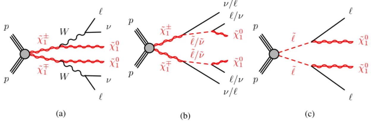
1 either via emission of a W boson, which may decay to an electron or muon plus neutrino(s) either directly or through the emission of a leptonically decaying τ lepton (see Figure 1(a)), or to a slepton-neutrino/sneutrino-lepton pair (see Figure 1(b)). In the latter case it is assumed that the scalar partners of the left-handed charged leptons and neutrinos are also light and thus accessible in the sparticle decay chains. It is also assumed they are mass-degenerate, and their masses are chosen to be midway between the mass of the chargino and that of the ˜ χ 0
1 , which is pure bino. Equal branching ratios for the three slepton flavours are assumed and charginos decay to charged sleptons or sneutrinos with a branching ratio of 50% to each. Lepton flavour is conserved in all models.
In models with direct ˜ ` ` ˜ production (see Figure 1(c)), each slepton decays into a lepton and a ˜ χ 0
1 with a 100% branching ratio. Only ˜ e and ˜ µ are considered in this model, and ˜ e L , ˜ e R , ˜ µ L and ˜ µ R are assumed to
be mass-degenerate.
(a)
˜ ± 1
˜ ⌥ 1
`/˜ ˜ ⌫
`/˜ ˜ ⌫ p
p
⌫/`
`/⌫
˜ 0 1
⌫/`
`/⌫
˜ 0 1
(b) (c)
Figure 1: Diagrams of the supersymmetric models considered in this paper, with two leptons and weakly interacting particles in the final state: (a) ˜ χ +
1 χ ˜ −
1 production with W boson mediated decays, (b) ˜ χ +
1 χ ˜ −
1 production with slepton/sneutrino-mediated decays and (c) slepton pair production. In the model with intermediate sleptons, all three flavors ( ˜ e , ˜ µ , ˜ τ ) are included, while only ˜ e and ˜ µ are included in the direct slepton model. In the final state, ` stands for an electron or muon, which can be produced directly or, in the case of (a) and (b) only, via a leptonically decaying τ with additional neutrinos.
3 ATLAS detector
The ATLAS detector [31] at the LHC is a general purpose detector with a forward-backward symmetric cylindrical geometry and an almost complete coverage in solid angle around the collision point. 1 It consists of an inner tracking detector surrounded by a thin superconducting solenoid, electromagnetic and hadronic calorimeters, and a muon spectrometer incorporating three large superconducting toroid magnets. The inner-detector system (ID) is immersed in a 2 T solenoidal axial magnetic field and provides charged
1 ATLAS uses a right-handed coordinate system with its origin at the nominal interaction point (IP) in the centre of the detector and the z -axis along the beam pipe. The x -axis points from the IP to the centre of the LHC ring, and the y -axis points upwards.
Cylindrical coordinates ( r, φ ) are used in the transverse plane, φ being the azimuthal angle around the z-axis. The pseudorapidity
is defined in terms of the polar angle θ as η = − ln tan (θ/ 2 ) . Rapidity is defined as y = 0 . 5 ln [(E + p z )/(E − p z )] , where E and
p z denote the energy and the component of the particle momentum along the beam direction, respectively.
particle tracking in the range |η | < 2 . 5. It consists of a high-granularity silicon pixel detector, a silicon microstrip tracker and a transition radiation tracker, which enables radially extended track reconstruction up to |η| = 2 . 0. The transition radiation tracker also provides electron identification information. During the first LHC long shutdown, a new tracking layer, known as the Insertable B-Layer (IBL) [32], was added with an average sensor radius of 33 mm from the beam pipe in order to improve tracking and b -tagging performance. The calorimeter system covers the pseudorapidity range |η| < 4 . 9. Within the region
|η| < 3 . 2, electromagnetic calorimetry is provided by barrel and endcap high-granularity lead/liquid-argon (LAr) electromagnetic sampling calorimeters. Hadronic calorimetry is provided by an iron/scintillating-tile sampling calorimeter within |η| < 1 . 7, and two copper/LAr hadronic endcap calorimeters. The solid angle coverage is completed with forward copper/LAr and tungsten/LAr calorimeter modules optimised for electromagnetic and hadronic measurements respectively. The muon spectrometer (MS) comprises separate trigger and high-precision tracking chambers measuring the deflection of muons in a magnetic field generated by superconducting air-core toroids. The precision chamber system covers the region
|η| < 2 . 7 with three layers of monitored drift tubes, complemented by cathode strip chambers in the forward region, where the background is higher. The muon trigger system covers the range |η | < 2 . 4 with resistive plate chambers in the barrel, and thin gap chambers in the endcap regions. A two-level trigger system is used to select events. There are a low-level hardware trigger implemented in custom electronics, which reduces the incoming data rate to a design value of 100 kHz using a subset of detector information, and a high-level software trigger which selects interesting final state events with algorithms accessing the full detector information, and further reduces the rate to about 1 kHz [33] .
4 Data and simulated event samples
The analysis described in this paper uses the 2015-2018 data collected by the ATLAS detector during pp collisions at a centre-of-mass energy of
√ s = 13 TeV. The average number hµi of additional pp interactions per bunch crossing (pileup) ranged between 14 in 2015 and about 38 in 2017-2018. After data-quality requirements, the data sample amounts to a total integrated luminosity of 139 fb − 1 collected in 2015-2018.
The uncertainty in the combined 2015-2018 integrated luminosity is 1.7%. It is derived from the calibration of the luminosity scale using x - y beam-separation scans, following a methodology similar to that detailed in Ref. [34], and using the LUCID-2 detector for the baseline luminosity measurements [35].
Events considered in this analysis must pass a trigger selection requiring at least two leptons of either electron or muon flavour. The trigger-level thresholds on the p T of the leptons involved in the trigger decision are different according to the data taking periods. They are in the range 8-22 GeV for data collected in 2015 and 2016, and 8-24 GeV for data collected in 2017 and 2018. These thresholds are looser than those applied in the lepton offline selection to ensure that trigger efficiencies are constant in the relevant phase space.
Simulated event samples are used for the SM background estimate and to model the SUSY signal. The MC
samples are processed through an ATLAS detector simulation [36] based on Geant4 [37] or a fast simulation
using a parametrisation of the ATLAS calorimeter response and Geant4 for the other components of the
detector [36]. They are reconstructed with the same algorithms as those used for the data. To compensate
for differences between data and simulation in the lepton reconstruction efficiency, energy scale and energy
resolution, in the b -tagging efficiency and in the modelling of the trigger [38, 39], correction factors are
derived from data and applied as weights to the simulated events.
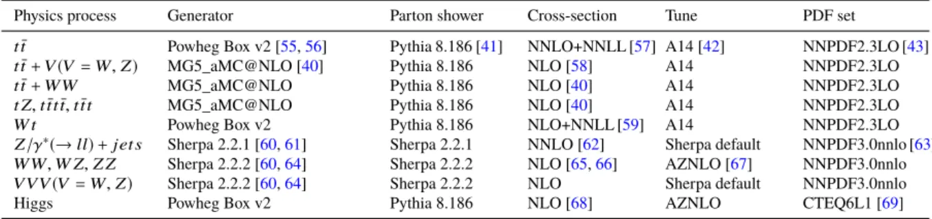
All SM backgrounds used are listed in Table 1 along with the relevant parton distribution function (PDF) set, the configuration of underlying-event and hadronisation parameters (underlying-event tune), and the cross-section calculation order in α S used to normalise the event yields for these samples.
The SUSY signal samples are generated from leading order (LO) matrix elements with up to two extra partons using MadGraph5_aMC@NLO [40] interfaced to Pythia 8.186 [41], with the A14 tune [42], for the modelling of the SUSY decay chain, parton showering, hadronisation and the description of the underlying event. Parton luminosities are provided by the NNPDF23LO PDF set [43]. Jet-parton matching is performed following the CKKW-L prescription [44], with a matching scale set to one quarter of the mass of the pair-produced superpartner. Signal cross-sections are calculated to next-to-leading order (NLO) in α S adding the resummation of soft gluon emission at next-to-leading-logarithmic accuracy (NLO+NLL) [45–51]. The nominal cross-sections and their uncertainties are taken from an envelope of cross-section predictions using different PDF sets and factorisation and renormalisation scales, as described in Ref. [52]. The cross-section for ˜ χ +
1 χ ˜ −
1 production, each with a mass of 400 GeV, is 58 . 6 ± 4 . 7 fb, while the cross-section for ˜ ` ` ˜ production, each with a mass of 500 GeV, is 0 . 47 ± 0 . 03 fb for each generation of left-handed sleptons and 0 . 18 ± 0 . 01 fb for each generation of right-handed sleptons.
Minimum-bias interactions are generated and overlaid on top of the hard-scattering process to simulate the effect of multiple pp interactions occurring during the same (in-time) or a nearby (out-of-time) bunch-crossing. These are produced using Pythia 8.186 with the A3 tune [53] and the MSTW2008LO PDF [54] set. The MC samples are reweighted so that the distribution of the average number of interactions per bunch-crossing matches the observed distribution in the data.
Table 1: Simulated background event samples used in this analysis with the corresponding matrix element and parton shower generators, cross-section order in α S used to normalise the event yield, underlying-event tune and PDF set.
Physics process Generator Parton shower Cross-section Tune PDF set
t¯ t Powheg Box v2 [55, 56] Pythia 8.186 [41] NNLO+NNLL [57] A14 [42] NNPDF2.3LO [43]
t¯ t + V (V = W, Z) MG5_aMC@NLO [40] Pythia 8.186 NLO [58] A14 NNPDF2.3LO
t¯ t + W W MG5_aMC@NLO Pythia 8.186 NLO [40] A14 NNPDF2.3LO
t Z, t¯ tt¯ t, t tt ¯ MG5_aMC@NLO Pythia 8.186 NLO [40] A14 NNPDF2.3LO
W t Powheg Box v2 Pythia 8.186 NLO+NNLL [59] A14 NNPDF2.3LO
Z/γ ∗ (→ ll) + jet s Sherpa 2.2.1 [60, 61] Sherpa 2.2.1 NNLO [62] Sherpa default NNPDF3.0nnlo [63]
W W, W Z, Z Z Sherpa 2.2.2 [60, 64] Sherpa 2.2.2 NLO [65, 66] AZNLO [67] NNPDF3.0nnlo VVV (V = W, Z) Sherpa 2.2.2 [60, 64] Sherpa 2.2.2 NLO Sherpa default NNPDF3.0nnlo
Higgs Powheg Box v2 Pythia 8.186 NLO [68] AZNLO CTEQ6L1 [69]
5 Object identification
Leptons selected for analysis are categorised as baseline or signal leptons according to various quality and kinematic selection criteria. Baseline objects are used in the calculation of missing transverse momentum, to resolve ambiguities between the analysis objects in the event and in the fake/non-prompt (FNP) lepton background estimation described in Section 7. Leptons used for the final event selection must pass more stringent signal requirements.
Baseline electron candidates are reconstructed using energy clusters in the electromagnetic calorimeter
which are matched to an ID track. They are required to pass a Loose likelihood-based identification
requirement [70], to have a transverse momentum p T > 10 GeV and to reside within the pseudorapidity
region |η | < 2 . 47. They are also required to be within |z 0 sin θ | = 0.5 mm of the primary vertex 2 , where z 0 is the longitudinal impact parameter with respect to the primary vertex. Signal electrons are required to satisfy a Tight identification requirement [70] and the track associated with the signal electron must have a significance of the transverse impact parameter with respect to the reconstructed primary vertex, d 0 , of
| d 0 |/σ(d 0 ) < 5.
Baseline muon candidates are reconstructed in the pseudorapidity region |η| < 2 . 7 from muon spectrometer tracks matching ID tracks. They are required to have p T > 10 GeV, to be within |z 0 sin θ | = 0.5 mm of the primary vertex and to satisfy the Medium identification requirements defined in Ref. [39]. The Medium identification criterion defines requirements on the number of hits in the different ID and muon spectrometer subsystems, and on the significance of the charge to momentum ratio q/p . Finally, the track associated with the signal muon must have |d 0 |/σ(d 0 ) < 3.
Isolation criteria are applied to signal electrons and muons. The scalar sum of the p T of tracks within a variable-size cone around the lepton (excluding its own track), must be less than 15% of the lepton p T . The track isolation cone radius for electrons (muons) ∆R = p
(∆ η) 2 + (∆ φ) 2 is given by the smaller of
∆R = 10 GeV /p T and ∆R = 0 . 2 ( 0 . 3 ) . In addition for electrons (muons) the sum of the transverse energy of the calorimeter energy clusters in a cone of ∆R = 0 . 2 around the lepton (excluding the deposit from the lepton itself) must be less than 20% (30%) of the lepton p T . For electrons with p T > 200 GeV these isolation requirements are not applied, and instead an upper limit of max(0 . 015 × p T , 3.5 GeV) is placed on the transverse energy of the calorimeter energy clusters in a cone of ∆R = 0 . 2 around the electron.
Jets are reconstructed from topological energy clusters in the calorimeter [71] using the anti- k t jet clustering algorithm [72] with a radius parameter R = 0 . 4. The reconstructed jets are then calibrated by the application of a jet energy scale (JES) derived from 13 TeV data and simulation [73]. Only jet candidates with p T > 20 GeV and |η | < 2 . 4 are considered as selected jets in the analysis 3 , although jets with |η| < 4 . 9 are included in the missing transverse momentum estimate and are considered when applying the procedure to remove reconstruction ambiguities later described in this section.
In order to reduce the effects of pileup, for jets with |η| ≤ 2 . 5 and p T < 120 GeV a significant fraction of the tracks associated with each jet must have an origin compatible with the primary vertex, as defined by the jet vertex tagger [74]. This requirement reduces jets from pileup to 1%, with an efficiency for pure hard scatter jets of about 90%. For jets with |η| > 2 . 5 and p T < 60 GeV pileup suppression is achieved through the forward jet vertex tagger [75] which exploits topological correlations between jet pairs. Finally, events containing a jet that does not pass jet quality requirements [76, 77] are vetoed in order to remove events impacted by detector noise and non-collision backgrounds.
The MV2C10 boosted decision tree algorithm [78, 79] identifies jets containing b -hadrons (“ b -tagged jets”, or “ b -jets” for short) by using quantities such as the impact parameters of associated tracks and positions of any good reconstructed secondary vertices. A selection that provides 85% efficiency for tagging b -jets in simulated t¯ t events is used. The corresponding rejection factors against jets originating from c -quarks, from τ -leptons, and from light quarks and gluons in the same sample at this working point are 3.1, 8.2 and 33, respectively.
To avoid the double counting of analysis baseline objects, a procedure to remove reconstruction ambiguities is applied as follows:
2 The primary vertex is defined as the vertex with the highest scalar sum of the squared transverse momentum of associated tracks with p T > 500 MeV.
3 Hadronic τ objects are treated as jets in this analysis.
• jet candidates within ∆R 0 = p
∆y 2 + ∆φ 2 < 0.2 of an electron candidate are removed;
• jets with fewer than three tracks which lie within ∆R 0 = 0 . 4 around a muon candidate are removed;
• electrons and muons within ∆R 0 = 0 . 4 of the remaining jets are discarded, in order to reject leptons from the decay of a b - or c -hadron;
• electron candidates are rejected if they are found to share an ID track with a muon.
The missing transverse momentum ( p miss
T ), which has magnitude E miss
T , is defined as the negative vector sum of the transverse momenta of all identified physics objects (electrons, photons, muons, jets). Low momentum contributions from particle tracks from the primary vertex which are not associated with reconstructed analysis objects (soft term) are also included in the calculation, and the E miss
T value is adjusted for the calibration of the selected physics objects [80]. Linked to the E miss
T value is the E miss
T significance value, which helps to separate events with true E miss
T (arising from weakly interacting particles) from those where it is consistent with particle mis–measurement, resolution or identification inefficiencies, as further detailed in Ref. [81].
6 Search strategy
Events used in this search are required to have exactly two oppositely-charged signal leptons ` 1 and ` 2 , both with p T > 25 GeV. In order to remove contributions from low-mass resonances and to ensure good modelling of the SM background in all regions relevant for the analysis, the invariant mass of the two leptons must be m `
1 ` 2 > 100 GeV. Events are further required to have no reconstructed b -jets, to suppress contributions from processes with top quarks. Selected events must also satisfy E miss
T > 110 GeV and E miss
T
significance > 10.
The stransverse mass m T2 [82, 83] is a kinematic variable used to bound the masses of a pair of particles that are presumed to have each decayed semi-invisibly into one visible and one invisible particle. It is defined as
m T2 (p T , 1 , p T , 2 , q T ) = min
q T,1 + q T,2 = q T
max [ m T (p T , 1 , q T , 1 ), m T (p T , 2 , q T , 2 ) ] , (1)
where m T indicates the transverse mass 4 , p T , 1 and p T , 2 are the transverse-momentum vectors of the two leptons, and q T , 1 and q T , 2 are vectors with p miss
T = q T , 1 + q T , 2 . The minimisation is performed over all the possible decompositions of q T . For t t ¯ or WW decays, assuming an ideal detector with perfect momentum resolution, m T2 (p T ,`
1 , p T ,` 2 , p miss
T ) has a kinematic endpoint at the mass of the W boson [83]. Signal models with sufficient mass splittings between the ˜ χ ±
1 and the ˜ χ 0
1 feature m T2 distributions that extend beyond the kinematic endpoint expected for the dominant SM backgrounds. Therefore, events in this search are required to have high m T2 values.
Events are separated into “same flavour” (SF) events, i.e. e ± e ∓ and µ ± µ ∓ , and “different flavour” (DF) events, i.e. e ± µ ∓ , with the split being motivated by different background compositions in the two classes of events. SF events are required to have a di-lepton invariant mass far away from the Z peak, asking for m ` 1 ` 2 > 121 . 2 GeV, to reduce diboson and Z +jets backgrounds.
4 The transverse mass is defined by m T = p
2 × | p T , 1 | × | p T , 2 | × ( 1 − cos (∆φ )) , where ∆φ is the difference in azimuthal angle
between the particles with transverse momenta p T ,1 and p T,2
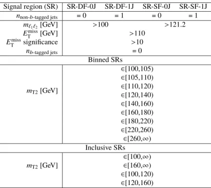
Events are further classified by the multiplicity of non- b -tagged jets ( n non- b -tagged jets ), i.e. the number of jets not identified as b -jets by the MV2C10 boosted decision tree algorithm. All events are required to have no more than one non- b -tagged jet. Following the classification of the events, two sets of signal regions (SRs) are defined: a set of exclusive, “binned” SRs, to maximise model-dependent exclusion sensitivity, and a set of “inclusive” SRs, to be used for model independent results. Among the second set of SRs two are fully inclusive, with a different lower bound in m T2 to target different chargino or slepton mass regions, while two have both lower and upper bounds on m T2 to target models with lower endpoints. The definitions of these regions are provided in Table 2. Each SR is identified by the lepton flavour combination (DF or SF), the number of non- b -tagged jets (0J,1J) and the range of the m T2 interval.
Signal region (SR) SR-DF-0J SR-DF-1J SR-SF-0J SR-SF-1J
n non- b -tagged jets = 0 = 1 = 0 = 1
m ` 1 ` 2 [GeV] > 100 > 121.2 E miss
T [GeV] > 110
E miss
T significance > 10
n b-tagged jets = 0
Binned SRs
m T2 [GeV]
∈ [100,105)
∈ [105,110)
∈ [110,120)
∈ [120,140)
∈ [140,160)
∈ [160,180)
∈ [180,220)
∈ [220,260)
∈ [260, ∞ ) Inclusive SRs
m T2 [GeV]
∈ [100, ∞ )
∈ [160, ∞ )
∈ [100,120)
∈ [120,160)
Table 2: The definitions of the binned and inclusive signal regions. Relevant kinematic variables are defined in the text. The bins labelled “DF”or “SF” refer to signal regions with different lepton flavour or same lepton flavour pair combinations, respectively, and the “0J” and “1J” labels refer to the non- b -tagged jets multiplicity.
7 Background estimation and validation
The SM backgrounds can be classified into irreducible backgrounds, from processes with prompt leptons and genuine E miss
T from neutrinos, and reducible backgrounds, which contain one or more FNP leptons.
The main irreducible backgrounds in this search come from SM diboson ( WW , W Z , Z Z ) and top-quark ( t¯ t
and Wt ) production. These are estimated using simulation, normalised using a simultaneous likelihood
fit to data (as described in Section 9) in dedicated control regions (CRs). The CRs are designed to be
enriched in the particular background process under study while remaining kinematically similar to the
SRs. The normalisations of the relevant backgrounds are then validated in a set of validation regions (VRs),
which are not used to constrain the fit, but are used to verify the agreement between data and predictions in
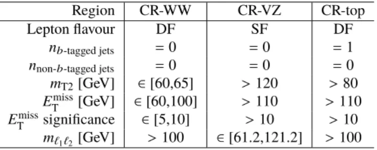
regions of the parameter space kinematically close to the SRs. Three CRs are used, as defined in Table 3:
CR-WW, targeting WW production; CR-top, targeting t t ¯ and single top-quark productions, which are normalised by using a single parameter in the likelihood fit to the data; and CR-VZ, targeting W Z and Z Z productions, which are also normalised by using a single parameter in the likelihood fit to the data.
Region CR-WW CR-VZ CR-top
Lepton flavour DF SF DF
n b -tagged jets = 0 = 0 = 1
n non- b -tagged jets = 0 = 0 = 0
m T2 [GeV] ∈ [60,65] > 120 > 80 E miss
T [GeV] ∈ [60,100] > 110 > 110 E miss
T significance ∈ [5,10] > 10 > 10 m ` 1 ` 2 [GeV] > 100 ∈ [61.2,121.2] > 100
Table 3: Control region definitions for extracting normalisation factors for the dominant background processes.
“DF”or “SF” refer to signal regions with different lepton flavour or same lepton flavour pair combinations, respectively.
The definitions of the VRs used in the analysis are provided in Table 4. For the WW background two validation regions are considered (VR-WW-0J and VR-WW-1J), according to the multiplicity of non- b - tagged jets in the event. As contributions from top-quark backgrounds in VR-WW-0J and VR-WW-1J are not negligible, three VRs are defined for this background. VR-top-low requires the same m T2 range as VR-WW-0J and VR-WW-1J, thus allowing the modelling of top-quark production at lower values of m T2 to be validated. VR-top-high requires m T2 > 100 GeV and provides validation in the high m T2 region where the SRs are also defined. Finally, VR-top-WW requires the same E miss
T , E miss
T significance and m T2 ranges as CR-WW and provides validation of the modelling of top-quark production in this region, where the contribution from top-quark backgrounds is relevant.
Region VR-WW-0J VR-WW-1J VR-VZ VR-top-low VR-top-high VR-top-WW
Lepton flavour DF DF SF DF DF DF
n b-tagged jets = 0 = 0 = 0 = 1 = 1 = 1
n non-b-tagged jets = 0 = 1 = 0 = 0 = 1 = 1
m T2 [GeV] ∈ [65,100] ∈ [65,100] ∈ [100,120] ∈ [80,100] > 100 ∈ [60,65]
E miss
T > 60 > 60 > 110 > 110 > 110 ∈ [60,100]
E miss
T significance > 5 > 5 > 10 ∈ [5,10] > 10 ∈ [5,10]
m ` 1 ` 2 [GeV] > 100 > 100 ∈ [61.2,121.2] > 100 > 100 > 100 Table 4: Validation region definitions used to study the modelling of the SM backgrounds. “DF” or “SF” refer to regions with different lepton flavour or same lepton flavour pair combinations, respectively.
In order to obtain CRs and VRs of reasonable purity in WW production, VR-WW-0J and VR-WW-1J all require lower m T2 values than the SRs. To validate the tails of the m T2 distribution, a method similar to the one described in Ref. [29] is used. Three-lepton events, pure in W Z production, are selected by requiring the absence of b -tagged jets and the presence of one same-flavour opposite-sign (SFOS) lepton pair whose invariant mass is consistent with that of the Z -boson ( |m `
1 ` 2 − m Z | < 10 GeV). To avoid overlaps with portions of the phase space relevant for other searches, three-lepton events are also required to satisfy E miss
T ∈ [ 40 , 170 ] GeV. To emulate the signal regions of this analysis events are also required to have exactly 0 or 1 non- b -tagged jet. The transverse momentum of the lepton in the SFOS pair that has the same charge as the remaining lepton is added to the p miss
T vector, to mimic a neutrino. The m T2 value can then be
calculated using the remaining two leptons in the event. With this selection, good shape agreement for
the m T2 distribution is observed between data and simulation, and no additional systematic uncertainty is applied to the WW background at high m T2 .
Sub-dominant irreducible SM background contributions come from Z +jets, Drell-Yan, t t ¯ + V and Higgs boson production. These processes, jointly referred to as “Other backgrounds” are estimated directly from simulation using the samples described in Section 4. The remaining background from FNP leptons is estimated from data using the matrix method (MM) [84]. This method considers two types of lepton identification criteria: so-called “signal” leptons, corresponding to leptons passing the full analysis selection, and so-called “baseline” leptons, as defined in Section 5. Probabilities for prompt leptons satisfying the baseline selection to also satisfy the signal selection are measured as a function of lepton p T and η in dedicated regions enriched in Z -boson processes. Similar probabilities for FNP leptons are measured in events dominated by leptons from heavy flavour hadron decays and photon conversions. These probabilities are used in the MM to extract data-driven estimates for the FNP lepton background in the CRs, VRs, and SRs, looking at the numbers of observed events containing a pair of baseline leptons in which one of the two leptons, both or none of them pass the signal selection in a given region. To avoid double counting between the simulated samples used for background estimation and the FNP lepton background estimate provided by the MM, all simulated events containing one or more FNP leptons are removed.
The number of observed events in each CR, as well as the predicted yield of each SM process are reported in Table 5. For backgrounds whose normalisation is extracted by the likelihood fit, the yield expected from the simulation before the fit is also reported. After the fit, the central values of the total number of predicted events in the CRs match the data, as expected due to the normalisation procedure. The normalisation factors returned by the fit for the WW , t¯ t and single top-quark backgrounds, and W Z / Z Z backgrounds are 1 . 25 ± 0 . 13, 0 . 82 ± 0 . 06 and 1 . 18 ± 0 . 06. The shape of kinematic distributions is well reproduced by the
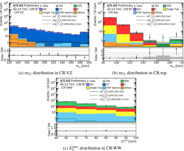
simulation in each CR. The distributions of m T2 in CR-VZ and CR-top and of E miss
T in CR-WW are shown in Figure 2.
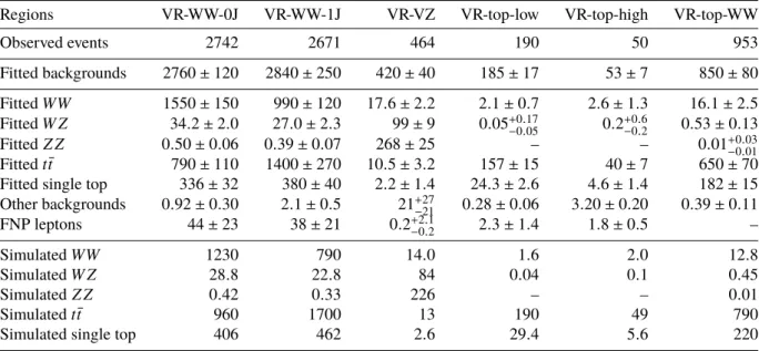
The observed number of events and the predicted background in each VR are reported in Table 6. For backgrounds whose normalisation is extracted from the fit, the expected yield from simulated samples before the fit is also reported. Figure 3 shows a selection of kinematic distributions for data and the estimated SM background in the validation regions defined in Table 4. Good agreement is observed in all regions.
8 Systematic uncertainties
All relevant sources of experimental and theoretical systematic uncertainty affecting the SM background estimates and the signal predictions are included in the likelihood fit described in Section 9. The dominant sources of systematic uncertainty are related to the theory uncertainties in the MC modelling, with the largest sources of experimental uncertainty being related to the jet energy scale (JES) and jet energy resolution (JER). The statistical uncertainty of the simulated event samples is also accounted for in the analysis. Since the normalisation of the predictions for the dominant background processes is extracted in dedicated control regions, the systematic uncertainties only affect the extrapolation to the signal regions in these cases.
The JES and JER uncertainties are considered as a function of jet p T and η , the pileup conditions and
the jet flavour composition of the selected jet sample. They are derived using a combination of data and
simulation, through measurements of the jet response balance in dijet, Z +jets and γ +jets events [85, 86].
Region CR-WW CR-VZ CR-top
Observed events 962 811 321
Fitted backgrounds 962 ± 31 811 ± 28 321 ± 18
Fitted WW 670 ± 60 19 . 1 ± 1 . 9 5 . 5 ± 2 . 7
Fitted W Z 11 . 8 ± 0 . 7 188 ± 7 0 . 32 ± 0 . 15
Fitted Z Z 0 . 29 ± 0 . 06 577 ± 23 –
Fitted t t ¯ 170 ± 50 1 . 8 ± 1 . 3 270 ± 16
Fitted single top 88 ± 8 0 . 65 ± 0 . 35 38 . 6 ± 2 . 6
Other backgrounds 0 . 17 ± 0 . 06 19 ± 7 2 . 21 ± 0 . 20
FNP leptons 21 ± 8 5 +6 − 5 4 . 2 ± 2 . 2
Simulated WW 528 15 . 1 4 . 3
Simulated W Z 9 . 9 158 0 . 27
Simulated Z Z 0 . 24 487 –
Simulated t t ¯ 210 2 . 2 327
Simulated single top 107 0 . 8 46 . 7
Table 5: Observed events and predicted background yields from the fit in the CRs. For backgrounds whose normalisation is extracted by the fit, the yield expected from the simulation before the fit is also reported. The background denoted as “Other” includes the non-dominant background sources for this analysis, i.e. Z +jets, t t ¯ + V , Higgs and Drell-Yan events. A “–” symbol indicates that the background contribution is negligible.
Regions VR-WW-0J VR-WW-1J VR-VZ VR-top-low VR-top-high VR-top-WW
Observed events 2742 2671 464 190 50 953
Fitted backgrounds 2760 ± 120 2840 ± 250 420 ± 40 185 ± 17 53 ± 7 850 ± 80 Fitted WW 1550 ± 150 990 ± 120 17 . 6 ± 2 . 2 2 . 1 ± 0 . 7 2 . 6 ± 1 . 3 16 . 1 ± 2 . 5 Fitted W Z 34 . 2 ± 2 . 0 27 . 0 ± 2 . 3 99 ± 9 0 . 05 +0.17 − 0.05 0 . 2 +0.6 − 0 . 2 0 . 53 ± 0 . 13 Fitted Z Z 0 . 50 ± 0 . 06 0 . 39 ± 0 . 07 268 ± 25 – – 0 . 01 +0 − 0.01 . 03 Fitted t t ¯ 790 ± 110 1400 ± 270 10 . 5 ± 3 . 2 157 ± 15 40 ± 7 650 ± 70 Fitted single top 336 ± 32 380 ± 40 2 . 2 ± 1 . 4 24 . 3 ± 2 . 6 4 . 6 ± 1 . 4 182 ± 15 Other backgrounds 0 . 92 ± 0 . 30 2 . 1 ± 0 . 5 21 +27 − 21 0 . 28 ± 0 . 06 3 . 20 ± 0 . 20 0 . 39 ± 0 . 11 FNP leptons 44 ± 23 38 ± 21 0 . 2 +2.1 − 0 . 2 2 . 3 ± 1 . 4 1 . 8 ± 0 . 5 –
Simulated WW 1230 790 14 . 0 1 . 6 2 . 0 12 . 8
Simulated W Z 28 . 8 22 . 8 84 0 . 04 0 . 1 0 . 45
Simulated Z Z 0 . 42 0 . 33 226 – – 0 . 01
Simulated t t ¯ 960 1700 13 190 49 790
Simulated single top 406 462 2 . 6 29 . 4 5 . 6 220
Table 6: Observed events and predicted background yields in the VRs. For backgrounds whose normalisation
is extracted from the fit in the CRs, the yield expected from the simulation before the fit is also reported. The
background denoted as “Other” includes the non-dominant background sources for this analysis, i.e. Z +jets, t t ¯ + V ,
Higgs and Drell-Yan events. A “–” symbol indicates that the background contribution is negligible.
[GeV]
mT2
Events / 20 GeV
1 10 10
210
310
410
510
6ATLAS Preliminary
=13 TeV, 139 fb
-1s CR-VZ
Data SM WW
WZ ZZ t t
Single Top FNP leptons Others
)=(400,200) GeV 0χ∼1
±,
~l m(
)=(300,50) GeV 0
χ∼1
±, χ∼1 m(
)=(600,300,1) GeV 0
χ∼1
±,
~l
±, χ∼1 m(
[GeV]
m
T2120 140 160 180 200 220 240 260 280 300
Data / SM 0.5 1 1.5
(a) m T2 distribution in CR-VZ
[GeV]
mT2
Events / 20 GeV
1 10 10
210
310
4ATLAS Preliminary
=13 TeV, 139 fb
-1s CR-top
Data SM WW
WZ t t Single Top
FNP leptons Others
)=(400,200) GeV 0χ∼1
±,
~l m(
)=(300,50) GeV 0
χ∼1
±, χ∼1 m(
)=(600,300,1) GeV 0
χ∼1
±,
~l
±, χ∼1 m(
[GeV]
m
T280 100 120 140 160 180 200
Data / SM 1 2 3
(b) m T2 distribution in CR-top
[GeV]
miss ET
Events / 10 GeV
1 10 10
210
310
410
510
6ATLAS Preliminary
=13 TeV, 139 fb
-1s CR-WW
Data SM WW
WZ ZZ t t
Single Top FNP leptons Others
)=(400,200) GeV 0χ∼1
±,
~l m(
)=(300,50) GeV 0
χ∼1
±, χ∼1 m(
)=(600,300,1) GeV 0
χ∼1
±,
~l
±, χ∼1 m(
[GeV]
miss
E
T60 65 70 75 80 85 90 95 100
Data / SM 0.5 1 1.5 2
(c) E miss
T distribution in CR-WW
Figure 2: Distributions of m T2 in (a) CR-VZ and (b) CR-top and (c) distribution of E miss
T in CR-WW for data and the estimated SM backgrounds. The normalisation factors extracted from the corresponding CRs are used to rescale the t t ¯ , single top-quark, WW , W Z and Z Z backgrounds. The FNP lepton background is calculated using the data-driven matrix method. The uncertainty band includes all systematic and statistical sources and the final bin in each histogram includes the overflow. Distributions for three benchmark signal points are overlaid for comparison.
An additional uncertainty on p miss
T comes from the soft-term resolution and scale [87]. Uncertainties on the scale factors applied to the simulated samples to account for differences between data and simulation in the b -jet identification efficiency are also included. The remaining experimental systematic uncertainties, such as those in the lepton reconstruction efficiency, lepton energy scale and lepton energy resolution and differences between the trigger efficiencies in data and simulation are included and were found to be a few per mille in all channels. The re-weighting procedure (pileup re-weighting) applied to simulation to match the distribution of the number of reconstructed vertices observed in data results in a negligible contribution to the total systematic uncertainty.
Several sources of theoretical uncertainty in the modelling of the dominant backgrounds are considered.
Uncertainties in the MC modelling of diboson events are estimated by varying the PDF sets as well as
the renormalisation and factorisation scales used to generate the samples. In order to account for the
effects due to the generator choice, the nominal Powheg diboson samples are compared with Sherpa
diboson samples which have a different matrix element calculation and parton shower simulation. For t¯ t
production, uncertainties from the parton shower simulation are accounted for by comparing samples with
Powheg interfaced to either Pythia 8.186 or Herwig++ [88, 89]. Another source of uncertainty comes
Region SR-DF-0J SR-DF-1J SR-SF-0J SR-SF-1J
m T2 [GeV] ∈ [100, ∞ ) ∈ [100, ∞ ) ∈ [100, ∞ ) ∈ [100, ∞ )
Total background expectation 97 75 144 124
Total systematic uncertainties 15% 12% 8% 10%
MC statistical uncertainties 3% 3% 2% 3%
WW normalisation 7% 6% 4% 3%
V Z normalisation < 1% < 1% 1% 1%
t¯ t normalisation 1% 2% < 1% 1%
Diboson theoretical uncertainties 7% 7% 4% 3%
Top theoretical uncertainties 7% 8% 3% 6%
E miss
T modelling 1% 1% < 1% 2%
Jet energy scale 2% 3% 2% 2%
Jet energy resolution 1% 2% 1% 2%
Pileup reweighting < 1% 1% < 1% < 1%
b -tagging < 1% 2% < 1% 1%
Lepton modelling 1% 1% 1% 3%
FNP leptons < 1% 1% 1% 1%
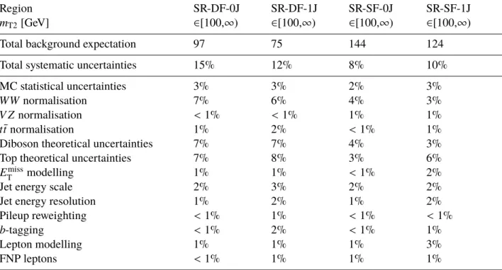
Table 7: Breakdown of the dominant systematic uncertainties on background estimates in the inclusive SRs requiring m T2 >100 GeV after performing the profile likelihood fit. Note that the individual uncertainties can be correlated, and do not necessarily add up quadratically to the total background uncertainty. The percentages show the size of the uncertainty relative to the total expected background. “Top theoretical uncertainties” refers to t t ¯ theoretical uncertainties and the uncertainty associated to Wt − t t ¯ interference added quadratically.
from the modelling of initial and final state radiation, which is calculated by comparing the predictions of the nominal sample with two alternative samples generated with Powheg interfaced to Pythia 8.186 but with the radiation settings varied [90]. The uncertainty associated to the choice of the event generator is estimated by comparing the nominal samples with samples generated with aMC@NLO interfaced to Pythia 8.186 [91]. Finally, for single top-quark production an uncertainty is associated to the treatment of the interference between the Wt and t t ¯ samples. This is done by comparing the nominal sample generated using the diagram removal method to a sample generated using the diagram subtraction method [90].
There are several contributions to the uncertainty on the matrix method estimate of the FNP background.
First an uncertainty is included from the observed differences in the probabilities for prompt leptons to satisfy the signal selection in simulation and data. Furthermore uncertainties on the expected composition of the FNP leptons in the signal regions are added. Finally, uncertainties from the limited statistics and on the subtraction of real lepton contamination in the control regions used to derive the probabilities for baseline leptons to pass signal requirements are considered.
A summary of the impact of the systematic uncertainties on the background yields in the inclusive SRs
with m T2 > 100 GeV, after performing the likelihood fit, is shown in Table 7. For the binned SRs defined
in Table 2, the uncertainties associated with limited MC statistics are higher.
9 Results
The statistical interpretation of the final results is performed using the HistFitter framework [92]. A simultaneous likelihood fit is performed which includes either the just the CRs (in the case of the background-only fit) or the CRs and one or more of the SRs (when calculating exclusion limits). The likelihood is a product of Poisson probability density functions describing the observed number of events in each CR/SR and Gaussian distributions that constrain the nuisance parameters associated with the systematic uncertainties. Poisson distributions are used for MC statistical uncertainties. Correlations of systematic uncertainties across samples are accounted for in the fit configuration by using the same nuisance parameter.
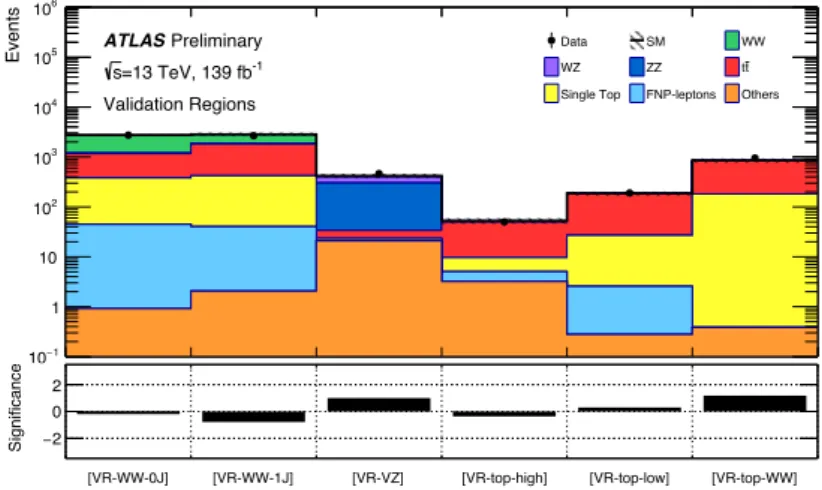
A background-only fit which uses data in the CRs only is performed to constrain the nuisance parameters of the likelihood function, which include the background normalisation factors and parameters associated with the systematic uncertainties. The results of the background-only fit are used to assess agreement between the data and background estimates in the validation regions. A good agreement, within about one standard deviation for all VRs, is observed, as shown in Section 7 and in Figure 4.
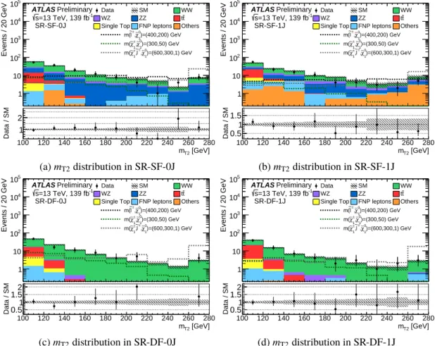
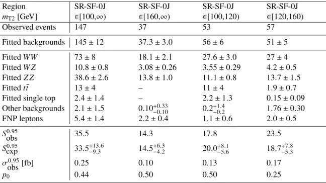
The results of the background-only fit in the CRs together with the observed data for the binned SRs are shown in Figure 5. The observed and the predicted number of background events in the inclusive SRs are reported in Tables 8 and 9. Figure 6 shows the m T2 distribution for the data and the estimated SM backgrounds for events in the SRs.
No significant deviation from the SM expectations is observed in any of the considered SRs, as shown in Figures 5 and 6. The CLs prescription [94] is used to set model-independent upper limits at 95%
confidence level (CL) on the visible signal cross-section σ 0 . 95
obs , defined as cross-section times acceptance times efficiency, of beyond the SM physics processes. They are derived in each inclusive SR by performing a fit which includes the observed yield in the SR as a constraint, and a free signal yield in the SR as parameter of interest. The observed ( S 0 . 95
obs ) and expected ( S exp 0 . 95 ) number of events from processes beyond the SM in the inclusive SRs defined in Section 6 are calculated. The p 0 -values, which represent the probability of the SM background alone to fluctuate to the observed number of events or higher, are also provided and are capped at p 0 = 0 . 50. These results are presented in Tables 8 and 9 for the SF and DF inclusive SRs, respectively.
Exclusion limits at 95% CL are set on the masses of the chargino, neutralino and sleptons for the simplified models in Figure 1. These also use the CLs prescription and include the exclusive SRs and the CRs in the simultaneous likelihood fit. For the models of chargino pair production the SF and DF SRs are included, whilst for direct slepton production only the SF SRs are included in the likelihood fit. The results are shown in Figure 7. In the model of direct chargino pair production with decays via W boson and for a massless
χ ˜ 0
1 , ˜ χ ±
1 masses up to 420 GeV are excluded at 95% CL. In the model of direct chargino pair production with decays via sleptons or sneutrinos and for a massless ˜ χ 0
1 , ˜ χ ±
1 masses up to 1 TeV are excluded at 95%
CL. Finally, in the model of direct slepton pair production and for a massless ˜ χ 0
1 , masses up to 700 GeV are
excluded at 95% CL.
[GeV]
mT2
Events / 10 GeV
1 10 10
210
310
410
510
6ATLAS Preliminary
=13 TeV, 139 fb
-1s VR-top-low
Data SM WW
WZ t t Single Top
FNP leptons Others )=(400,200) GeV
0
χ∼
1±
,
~ l m(
)=(300,50) GeV
0
χ∼
1±
, χ∼
1m(
)=(600,300,1) GeV
0
χ∼
1±
,
~ l
±
, χ∼
1m(
[GeV]
m
T280 82 84 86 88 90 92 94 96 98 100
Data / SM 0.5 1 1.5 2
(a) m T2 distribution in VR-top-low
[GeV]
mT2
Events / 25 GeV
1 10 10
210
3ATLAS Preliminary
=13 TeV, 139 fb
-1s
VR-top-high
Data SM WW
WZ t t Single Top
FNP leptons Others )=(400,200) GeV
0
χ∼
1±
,
~ l m(
)=(300,50) GeV
0
χ∼
1±
, χ∼
1m(
)=(600,300,1) GeV
0
χ∼
1±
,
~ l
±
, χ∼
1m(
[GeV]
m
T2100 120 140 160 180 200 220 240
Data / SM 0.5 1 1.5 2
(b) m T2 distribution in VR-top-high
[GeV]
miss ET
Events / 40 GeV
1 10 10
210
310
410
510
6ATLAS Preliminary
=13 TeV, 139 fb
-1s VR-WW-0J
Data SM WW
WZ ZZ t t
Single Top FNP leptons Others )=(400,200) GeV
0
χ∼
1±
,
~ l m(
)=(300,50) GeV
0
χ∼
1±
, χ∼
1m(
)=(600,300,1) GeV
0
χ∼
1±
,
~ l
±
, χ∼
1m(
[GeV]
miss
E
T100 150 200 250 300 350 400
Data / SM 0.5 1 1.5 2
(c) E miss
T distribution in VR-WW-0J
[GeV]
miss ET
Events / 40 GeV
1 10 10
210
310
410
510
6ATLAS Preliminary
=13 TeV, 139 fb
-1s VR-WW-1J
Data SM WW
WZ ZZ t t
Single Top FNP leptons Others )=(400,200) GeV
0
χ∼
1±
,
~ l m(
)=(300,50) GeV
0
χ∼
1±
, χ∼
1m(
)=(600,300,1) GeV
0
χ∼
1±
,
~ l
±
, χ∼
1m(
[GeV]
miss
E
T100 150 200 250 300 350 400
Data / SM 0.5 1 1.5 2
(d) E miss
T distribution in VR-WW-1J
significance miss ET
Events / 2.5
1 10 10
210
310
410
510
6ATLAS Preliminary
=13 TeV, 139 fb
-1s VR-VZ
Data SM WW
WZ ZZ t t
Single Top FNP leptons Others )=(400,200) GeV
0
χ∼
1±
,
~ l m(
)=(300,50) GeV
0
χ∼
1±
, χ∼
1m(
)=(600,300,1) GeV
0
χ∼
1±
,
~ l
±
, χ∼
1m(
significance
miss
E
T10 11 12 13 14 15 16 17 18 19 20
Data / SM 0.5 1 1.5 2
(e) E miss
T significance distribution in VR-VZ
significance miss ET
Events / 1.25
1 10 10
210
310
410
510
610
7ATLAS Preliminary
=13 TeV, 139 fb
-1s
VR-top-WW
Data SM WW
WZ ZZ t t
Single Top FNP leptons Others )=(400,200) GeV
0
χ∼
1±
,
~ l m(
)=(300,50) GeV
0
χ∼
1±
, χ∼
1m(
)=(600,300,1) GeV
0
χ∼
1±
,
~ l
±
, χ∼
1m(
significance
miss
E
T5 5.5 6 6.5 7 7.5 8 8.5 9 9.5 10
Data / SM 0.5 1 1.5
(f) E miss
T significance distribution in VR-top-WW Figure 3: Distributions of m T2 in (a) VR-top-low and (b) VR-top-high, E miss
T in (c) VR-WW-0J and (d) VR-WW-1J, and E miss
T significance in (e) VR-VZ and (f) VR-top-WW, for data and the estimated SM backgrounds. The
normalisation factors extracted from the corresponding CRs are used to rescale the t t ¯ , single top-quark, WW , W Z and
Z Z backgrounds. The FNP lepton background is calculated using the data-driven matrix method. The uncertainty
band includes all systematic and statistical sources and the last bin includes the overflow. Distributions for three
benchmark signal points are overlaid for comparison.
a[VR-WW-0J] b[VR-WW-1J] c[VR-VZ] d[VR-top-high] e[VR-top-low] f[VR-top-WW]
−1
10 1 10 10
210
310
410
510
6Events
Data SM WWWZ ZZ tt
Single Top FNP-leptons Others
Preliminary ATLAS
=13 TeV, 139 fb
-1s
Validation Regions
[VR-WW-0J] [VR-WW-1J] [VR-VZ] [VR-top-high] [VR-top-low] [VR-top-WW]
− 2 0 2
Significance
Figure 4: The upper panel reports the observed number of events in each of the VRs defined in Table 4, together with the expected SM backgrounds obtained after the background-only fit in the CRs. The shaded band represents the total uncertainty on the expected SM background. The lower panel reports the significance as defined in Ref. [93].
a[100,105)a[105,110)a[110,120)a[120,140)a[140,160)a[160,180)a[180,220)a[220,260)
∞)
a[260,b[100,105)b[105,110)b[110,120)b[120,140)b[140,160)b[160,180)b[180,220)b[220,260)
∞)
b[260,c[100,105)c[105,110)c[110,120)c[120,140)c[140,160)c[160,180)c[180,220)c[220,260)
∞)
c[260,d[100,105)d[105,110)d[110,120)d[120,140)d[140,160)d[160,180)d[180,220)d[220,260)
∞) d[260,
0
10 20 30 40 50
Events
Data SM WW
WZ ZZ tt
Single Top FNP-leptons Others
Preliminary
ATLAS
=13 TeV, 139 fb
-1s Signal Regions
[100,105) [105,110) [110,120) [120,140) [140,160) [160,180) [180,220) [220,260) )∞[260, [100,105) [105,110) [110,120) [120,140) [140,160) [160,180) [180,220) [220,260) )∞[260, [100,105) [105,110) [110,120) [120,140) [140,160) [160,180) [180,220) [220,260) )∞[260, [100,105) [105,110) [110,120) [120,140) [140,160) [160,180) [180,220) [220,260) )∞[260,
2
− 0 2
Significance
[GeV]
SR-DF-0J mT2 SR-DF-1J mT2 [GeV] SR-SF-0J mT2 [GeV] SR-SF-1J mT2 [GeV]
Figure 5: The upper panel reports the observed number of events in each of the SRs defined in Table 2, together with
the expected SM backgrounds obtained after the background-only fit in the CRs. The shaded band represents the
total uncertainty on the expected SM background. The lower panel reports the significance as defined in Ref. [93].
[GeV]
mT2
Events / 20 GeV
1 10 10
210
310
410
5ATLAS Preliminary
=13 TeV, 139 fb
-1s SR-SF-0J
Data SM WW
WZ ZZ t t
Single Top FNP leptons Others
)=(400,200) GeV 0χ∼1
±,
~l m(
)=(300,50) GeV 0
χ∼1
±, χ∼1 m(
)=(600,300,1) GeV 0
χ∼1
±,
~l
±, χ∼1 m(
[GeV]
m
T2100 120 140 160 180 200 220 240 260 280
Data / SM 1 2
(a) m T2 distribution in SR-SF-0J
[GeV]
mT2
Events / 20 GeV
1 10 10
210
310
410
5ATLAS Preliminary
=13 TeV, 139 fb
-1s SR-SF-1J
Data SM WW
WZ ZZ t t
Single Top FNP leptons Others
)=(400,200) GeV 0χ∼1
±,
~l m(
)=(300,50) GeV 0
χ∼1
±, χ∼1 m(
)=(600,300,1) GeV 0
χ∼1
±,
~l
±, χ∼1 m(
[GeV]
m
T2100 120 140 160 180 200 220 240 260 280
Data / SM 0.5 1 1.5
(b) m T2 distribution in SR-SF-1J
[GeV]
mT2
Events / 20 GeV
1 10 10
210
310
410
5ATLAS Preliminary
=13 TeV, 139 fb
-1s SR-DF-0J
Data SM WW
WZ ZZ t t
Single Top FNP leptons Others
)=(400,200) GeV 0χ∼1
±,
~l m(
)=(300,50) GeV 0
χ∼1
±, χ∼1 m(
)=(600,300,1) GeV 0
χ∼1
±,
~l
±, χ∼1 m(
[GeV]
m
T2100 120 140 160 180 200 220 240 260 280
Data / SM 0.5 1 1.5 2
(c) m T2 distribution in SR-DF-0J
[GeV]
mT2
Events / 20 GeV
1 10 10
210
310
410
5ATLAS Preliminary
=13 TeV, 139 fb
-1s SR-DF-1J
Data SM WW
WZ ZZ t t
Single Top FNP leptons Others
)=(400,200) GeV 0χ∼1
±,
~l m(
)=(300,50) GeV 0
χ∼1
±, χ∼1 m(
)=(600,300,1) GeV 0
χ∼1
±,
~l
±, χ∼1 m(