• Keine Ergebnisse gefunden

s = 13 TeV pp collisions √ b -taggedjetsusingtheATLASdetectorin Searchforpairproductionofhiggsinosinfinalstateswithatleastthree ATLASCONFNote

N/A
N/A
Protected

Academic year: 2021

Aktie "s = 13 TeV pp collisions √ b -taggedjetsusingtheATLASdetectorin Searchforpairproductionofhiggsinosinfinalstateswithatleastthree ATLASCONFNote"

Copied!
33
0
0

Wird geladen.... (Jetzt Volltext ansehen)

Volltext

(1)

A TLAS-CONF-2017-081 14 December 2017

ATLAS CONF Note

ATLAS-CONF-2017-081

12th December 2017

Search for pair production of higgsinos in final states with at least three b -tagged jets using the

ATLAS detector in

s = 13 TeV p p collisions

The ATLAS Collaboration

A search for pair production of the supersymmetric partners of the Higgs boson (higgsinos ˜ H ) in gauge-mediated scenarios is reported. Each higgsino is assumed to decay to a Higgs boson and a gravitino. Two complementary analyses, targeting high- and low-mass signals, are performed to maximize sensitivity. The analyses utilize LHC proton–proton collision data at a centre-of-mass energy

√ s = 13 TeV, the former with an integrated luminosity of 36.1 fb 1 and the latter with 24.3 fb 1 collected with the ATLAS detector in 2015 and 2016. The search is performed in events containing missing transverse momentum and several energetic jets, at least three of which must be identified as b -quark jets. No significant excess is found above the predicted background. Limits on the cross section are set as a function of the mass of the ˜ H in simplified models assuming production via mass-degenerate higgsinos decaying to a Higgs boson and the gravitino; higgsinos with mass between 130 GeV and 230 GeV and between 290 GeV and 880 GeV are excluded at 95% confidence level. An interpretation of the limits in terms of the branching ratio of the higgsino to Z boson or Higgs boson decays is also presented: a branching ratio to Higgs boson decays of 45% is excluded for m H ˜ ≈ 400 GeV.

© 2017 CERN for the benefit of the ATLAS Collaboration.

Reproduction of this article or parts of it is allowed as specified in the CC-BY-4.0 license.

(2)

1 Introduction

Supersymmetry (SUSY) [1–6] predicts new partners of the Standard Model (SM) particles: every boson is paired with a fermionic supersymmetric partner, and vice versa. Under the assumption of R -parity conservation [7], SUSY particles are produced in pairs and the lightest supersymmetric particle (LSP) is stable. If manifested in reality, SUSY would be a broken symmetry since the masses of the partner particles are not equal to those of the SM particles. The problem of the fine-tuning of the Higgs boson mass in the SM at the electroweak scale can be explained by the cancellation of divergent diagrams with their supersymmetric counterparts [8–11]. These “natural” SUSY models generally require light partners of the gluon (gluino), top quark (stop), and the Higgs boson itself (higgsinos, ˜ H 0

1 , ˜ H ± , ˜ H 0

2 ) [12]. Searches by the ATLAS and CMS collaborations have set strong limits on the masses of gluinos and stops in these scenarios, raising the prospect that the higgsino may be light enough to be the earliest SUSY particle to be detected.

This paper presents a search for the pair production of higgsinos in models of general gauge mediation (GGM) [13–17] or gauge-mediated symmetry breaking (GMSB) [18, 19] with a gravitino ( ˜ G ) LSP, where each higgsino decays to a Higgs boson and the gravitino, in the 4 b -jet + E miss

T final state. 1 SUSY predicts five different Higgs bosons; the observed Higgs boson at m h ≈ 125 GeV is assumed to be the light CP-even Higgs ( h ) of the MSSM [20]. The high branching fraction of the observed Higgs to a pair of b -jets makes this channel particularly sensitive to these models. The search is conducted using two complementary analyses targeting high- and low-mass higgsinos. The analysis targeting the high-mass signals uses 36.1 fb 1 of

√ s = 13 TeV pp collision data from the LHC recorded by the ATLAS detector [21] in 2015 and 2016 and utilizes E miss

T triggers which are efficient for high-mass higgsinos. For low-mass higgsinos the E miss

T is significantly reduced; to recover acceptance, a dedicated low-mass search inspired by the ATLAS di-Higgs resonance search [22] uses a combination of b -jet triggers in 24.3 fb 1 of data collected by the ATLAS detector in 2016. This is the first search performed by ATLAS for these signatures; CMS has reported a similar search at 8 TeV [23] and at 13 TeV [24].

The note is organized as follows. The SUSY models under scrutiny are described in Section 2, followed by a brief description of the ATLAS detector in Section 3. The datasets and simulated event samples are described in Section 4, and the object reconstruction is summarized in Section 5. The event selection and background estimation strategies are presented for the high-mass and low-mass analyses in Sections 6.1 and 6.2. The systematic uncertainties for both analyses are described in Section 7, and the results are shown in Section 8. Finally, the results are interpreted in the context of model-independent cross-section upper limits and as limits on simplified models of higgsino pair-production in Section 9, followed by a brief conclusion in Section 10.

2 SUSY signal models

In most realizations of supersymmetry, the higgsinos mix with gauginos (supersymmetric partners of the electroweak gauge bosons) to form mass eigenstates referred to as charginos ( ˜ χ ± ) and neutralinos ( ˜ χ 0 ).

Natural models often demand that the lightest neutralinos and charginos are dominated by the higgsino component; in this scenario the masses of the four lightest such particles, with mass ordering m χ ˜ 0

1

< m χ ˜ ± 1

1 E miss

T is the magnitude of the missing transverse momentum vector, which is the negative vectorial sum of the transverse

momenta ( p T ) of all visibleparticles in the event.

(3)

< m χ ˜ 0

2 , would be nearly degenerate [25–27]. In these models, sparticle production is dominated by the χ ˜ 0

1 χ ˜ 0

2 , ˜ χ 0

1 χ ˜ ±

1 , ˜ χ 0

2 χ ˜ ±

1 , and ˜ χ +

1 χ ˜

1 processes; in these scenarios, the heavier chargino and neutralinos can cascade decay to the lightest neutralino ( ˜ χ 0

1 ) via off-shell W and Z bosons, which are assumed to decay to immeasurably low momentum particles.

In SUSY models with low SUSY breaking scales, such as GGM or GMSB, a ˜ G is typically assumed to be the LSP; in natural models with light higgsinos, the ˜ χ 0

1 then becomes the next-to-lightest-supersymmetric (NLSP) particle. While a variety of decay scenarios are possible between the various higgsino states and the LSP, the models under study in this analysis assume that the heavier higgsinos decay first to the ˜ χ 0

1

and then promptly to the LSP. Depending on the specific parameters of the model, the ˜ χ 0

1 can decay to the G ˜ via a photon, Z boson, or Higgs boson [28]. If m H ˜ is greater than the Higgs mass, the ˜ χ 0

1 is dominated by the higgsino component, and tan β (the ratio of expectation values of the Higgs doublets) is small, then the dominant decay will typically be via Higgs bosons, which can in turn decay to pairs of b -quarks which this search targets.

These scenarios are implemented as simplified models [29–31] as shown in Figure 1. The primary free parameter of the model is the mass of the degenerate higgsino states, m H ˜ ; the mass of the LSP is set to a negligibly small value. Additionally, to study the effects of model parameters which affect the decay mode of the NLSP, the branching ratio of the ˜ χ 0

1 decays is varied between 100% h G ˜ and 100% Z G ˜ decays. The cross-section is set to the sum of the four mass-degenerate higgsino pair production processes.

H ˜

H ˜ h/Z

p h/Z p

G ˜ b b

G ˜

b b

Figure 1: Diagram for the simplified model considered in the analysis. The primary interpretation of the analysis is the decay via Higgs bosons, but decays via varied branching ratios to Z bosons are also studied. The production of the ˜ H occurs via mass-degenerate pairs of charginos or neutralinos, which decay to the ˜ χ 0

1 and immeasurably low momentum particles.

3 ATLAS detector

The ATLAS detector is a multipurpose particle detector with a forward-backward symmetric cylindrical geometry and nearly 4 π coverage in solid angle. 2 The inner tracking detector (ID) consists of silicon

2 ATLAS uses a right-handed coordinate system with its origin at the nominal interaction point in the center of the detector.

The positive x -axis is defined by the direction from the interaction point to the centre of the LHC ring, with the positive y -axis

pointing upwards, while the beam direction defines the z -axis. Cylindrical coordinates (r, φ) are used in the transverse plane, φ

being the azimuthal angle around the z-axis. The pseudorapidity η is defined in terms of the polar angle θ by η = − ln tan (θ/2 ) .

Rapidity is defined as y = 0 . 5 ln[ ( E + p z )/(E − p z ) ] where E denotes the energy and p z is the component of the momentum

along the beam direction.

(4)

pixel and microstrip detectors covering the pseudorapidity region |η | < 2 . 5, surrounded by a transition radiation tracker, which enhances electron identification in the region |η| < 2 . 0. Before the start of Run 2, the new innermost pixel layer, the insertable B-layer (IBL) [32], was inserted at a mean sensor radius of 3.3 cm. The ID is surrounded by a thin superconducting solenoid providing an axial 2 T magnetic field and by a fine-granularity lead/liquid-argon (LAr) electromagnetic calorimeter covering |η | < 3 . 2.

A steel/scintillator-tile calorimeter provides coverage for hadronic showers in the central pseudorapidity range ( |η | < 1 . 7). The endcaps (1 . 5 < |η | < 3 . 2) of the hadronic calorimeter are made of LAr active layers with either copper or tungsten as the absorber material. The forward region (3 . 1 < |η | < 4 . 9) is instrumented with a LAr calorimeter for both the EM and hadronic measurements. A muon spectrometer with an air-core toroidal magnet system surrounds the calorimeters. Three layers of high-precision tracking chambers provide coverage in the range |η | < 2 . 7, while dedicated fast chambers allow triggering in the region |η | < 2 . 4. The ATLAS trigger system [33] consists of a hardware-based level-1 trigger followed by a software-based high-level trigger (HLT).

4 Data and simulated event samples

The data used in this analysis were collected by the ATLAS detector from pp collisions produced by the LHC at a centre-of-mass-energy of 13 TeV and 25 ns proton bunch spacing over the 2015 and 2016 data- taking periods. The high-mass analyses uses data from 2015 corresponding to an integrated luminosity of 3.2 fb 1 and from 2016 with an integrated luminosity of 32.9 fb 1 , after the application of beam, detector and data-quality requirements. The low-mass analysis uses data from the 2016 dataset with an integrated luminosity of 24.3 fb 1 . The uncertainties on the integrated luminosities are found to be ± 2 . 1% and

± 2 . 2% for the 2015 and 2016 datasets, respectively, from a calibration of the luminosity scale using x – y beam-separation scans performed in August 2015 and May 2016, following a methodology similar to that detailed in Ref. [34]. The difference in luminosity between the analyses is the result of specific choices of triggers. In the high-mass analysis, events are required to pass an E miss

T trigger with thresholds of 70 GeV, 90 GeV, 100 GeV, and 110 GeV at the HLT level for the 2015, and early, mid, and late 2016 datasets, respectively. These triggers are fully efficient for events passing the preselection defined in Section 6.1, which requires the offline reconstructed E miss

T to exceed 200 GeV. In the low-mass analysis, a combination of b -jet triggers is used. These require either one or two b -tagged jets with p T thresholds of 35, 100 and 225 GeV and the presence of additional jets in the event. During 2016 data taking, a fraction of the data suffered from a faulty vertex reconstruction, and those events were not retained for further analysis. For the combined 2015 and 2016 dataset, there are on average 24 inelastic pp collisions per bunch crossing (the interactions other than the hard scatter are referred to as “pileup”).

Samples of Monte Carlo (MC) simulated events are used to model the signal and background processes in the high-mass analysis, except multijet processes, which are estimated from data. In the low-mass analysis, the background is dominated by multijet processes that are not modeled reliably in simulation, and the estimation methodology is thus based on data control samples as described in Section 6.2. SUSY signal samples are generated with up to two additional partons using MadGraph5_aMC@NLO [35] v2.3.3 at leading order (LO) with the NNPDF 2.3 [36] parton distribution function (PDF) set. These samples are interfaced to Pythia v8.186 [37] for the modeling of the parton showering, hadronization and underlying event.

The generators used to simulate signal processes for both analyses and background processes for the high-

mass analysis are described in Table 1. The dominant background is t¯ t production, which is simulated

(5)

Table 1: List of event generators used for the different processes. Information is given about the underlying-event tunes, the PDF sets and the pQCD highest-order accuracy used for the normalization of the different samples.

Process Event Generator Tune PDF set Cross-section

+ fragmentation/hadronization order

SUSY signal MadGraph5_aMC@NLO v2.3.3 A14 NNPDF2.3 NLO+NLL [41–46]

+ Pythia v8.186

t t ¯ Powheg-Box v2 PERUGIA2012 CT10 NNLO+NNLL [50]

+ Pythia v6.428

Single top Powheg-Box v1 or v2 PERUGIA2012 CT10 NNLO+NNLL [51–53]

+ Pythia v6.428

t ¯ tW/t ¯ t Z/4-tops MadGraph5_aMC@NLO v2.2.2 A14 NNPDF2.3 NLO [54]

+ Pythia v8.186

t t H ¯ MadGraph5_aMC@NLO v2.2.1 UEEE5 CT10 NLO [55]

+ Herwig++ v2.7.1

Diboson Sherpa v2.1.1 Default CT10 NLO [56]

W W , W Z , Z Z

W /Z+jets Sherpa v2.2.0 Default NNPDF3.0 NNLO [57]

with the Powheg-Box [38] v2 event generator. The W t - and s -channel production of single top quarks also use this generator, while t -channel is generated with Powheg-Box v1. Backgrounds from W/Z +jets processes are simulated using the Sherpa v2.2.0 [39] event generator, while Sherpa v2.1.1 is used to simulate diboson production processes. The production of t¯ t pairs in association with electroweak vector bosons W , Z , and Higgs bosons are modeled by samples generated using MadGraph5_aMC@NLO [40].

MadGraph5_aMC@NLO is also used to simulate the t¯ tt¯ t production. All details on the versions of the generators, showering models, tunes, and PDF sets are available in Table 1.

All background processes are initially normalized using the best available theoretical calculation for their respective cross-sections; the t¯ t contribution is further normalized using data as described in Section 6.1.

The order of this calculation in perturbative QCD for each process is listed in Table 1.

The signal samples are normalized using the best cross-section calculations at NLO in the strong coupling constant, adding the resummation of soft gluon emission at next-to-leading-logarithm (NLL) accuracy [41–45]. The generator, tune, and PDF are described in Table 1. The nominal cross-section and the uncertainty are taken from an envelope of cross-section predictions using different PDF sets and factorization and renormalization scales, as described in Ref. [46]. The cross-section of higgsino pair production at m H ˜ = 150 GeV is 3830 fb, while at m H ˜ = 900 GeV it is 1.8 fb.

All simulated event samples are passed through the full ATLAS detector simulation [47] using Geant4 [48],

with the exception of signal samples, which are passed through a fast simulation [49] that uses a para-

meterisation for the calorimeter response and Geant4 for the ID and the muon spectrometer. Pileup

collisions are simulated with Pythia 8 [37], and are overlaid on each MC event. Weights are assigned

to the simulated events such that the distribution of the number of pileup interactions in the simulation

matches the corresponding distribution in the data. The simulated events are reconstructed with the same

algorithm as that used for data.

(6)

5 Object reconstruction

Interaction vertices from the proton–proton collisions are reconstructed from at least two tracks with p T > 0 . 4 GeV, and are required to be consistent with the beamspot envelope. The primary vertex is identified as the one with the largest sum of squares of the transverse momenta from associated tracks ( P

|p T , track | 2 ) [58].

Jets are reconstructed from three-dimensional topological energy clusters [59] in the calorimeter using the anti- k t jet algorithm [60, 61] with a radius parameter of 0.4. Each topological cluster is calibrated to the electromagnetic scale response prior to jet reconstruction. The reconstructed jets are then calibrated to the particle level by the application of a jet energy scale (JES) derived from

√ s = 13 TeV data and simulations [62]. Quality criteria are imposed to reject events that contain at least one jet arising from non-collision sources or detector noise [63]. Further requirements are applied to reject jets with |η| < 2 . 4 that originate from pile-up interactions by means of a multivariate algorithm using information about the tracks matched to each jet [64]. Candidate jets are required to have p T > 20 GeV and |η| < 2 . 8 in the high-mass analysis and p T > 25 GeV and |η | < 2 . 5 in the low-mass analysis. After resolving overlaps with electrons and muons, as described below, selected jets are required to satisfy the stricter requirement of p T > 25 GeV in the high-mass analysis and 40 GeV in the low-mass analysis. The higher p T cut in the low-mass analysis is the result of the b -jet trigger thresholds.

A candidate jet is tagged as a b -jet by means of a multivariate algorithm using information about the impact parameters of inner detector tracks matched to the jet, the presence of displaced secondary vertices, and the reconstructed flight paths of b - and c -hadrons inside the jet [65, 66]. The b -tagging working point corresponding to an efficiency of 77% to identify b -jets with p T > 20 GeV, as determined from a sample of simulated t¯ t events, is found to be optimal in the high-mass analysis, while the low-mass analysis uses a tighter working point with 70% b -tagging efficiency in order to suppress the large contribution from light-flavor jets in the multijet background. The corresponding rejection factors against jets originating from c -quarks, τ -leptons and light quarks and gluons in the same sample for the selected working point are 6, 22 and 134, respectively, for the high-mass analysis and 12, 55 and 381, respectively, for the low-mass analysis.

Electron candidates are reconstructed from energy clusters in the electromagnetic calorimeter and inner detector tracks and are required to have |η| < 2.47 and satisfy a set of “loose” quality criteria [67, 68].

Muon candidates are reconstructed from matching tracks in the inner detector and muon spectrometer.

They are required to meet “medium” quality criteria, as described in Ref. [69], and to have |η| < 2.5. An isolation requirement is applied to both electrons and muons on the scalar sum of p T of additional inner detector tracks in a cone around the lepton track. This isolation requirement is defined to ensure a constant efficiency of around 99% across the whole electron transverse energy and muon transverse momentum ranges measured in Z → l + l events [67–69]. The angular separation between the lepton and the b -jet ensuing from a semileptonic top quark decay narrows as the p T of the top quark increases. This increased collimation is accounted for by setting the radius of the isolation cone to min(0.2, 10 GeV/ p lep

T ), where p lep

T

is the lepton p T expressed in GeV. In the high-mass analysis, the selected electrons are further required to meet the “tight” quality criteria [67, 68]. Leptons used in the calculation of E miss

T , in the four-momentum correction of b -tagged jets and to resolve overlaps among each other and with jets are required to have p T

> 5 GeV, while for vetoing events, the leptons are required to have p T > 20 GeV.

Overlaps between candidate objects are removed sequentially. If a reconstructed muon shares an ID track

with an electron, the electron is removed. In the high-mass analysis, any non- b -tagged jet whose axis

(7)

lies ∆R < 0 . 2 from an electron is removed. 3 Any electrons reconstructed within ∆R = min ( 0 . 4 , 0 . 04 + 10 GeV /p T ) of the axis of any surviving jet are removed. If a non- b -tagged jet is reconstructed within

∆R < 0 . 2 of a muon and the jet has fewer than three associated tracks or the muon energy constitutes most of the jet energy then the jet is removed. Muons reconstructed within a cone of size ∆R = min(0 . 4 , 0 . 04 + 10 GeV /p T ) around the jet axis of any surviving jet are removed. The same overlap procedure is applied in the low-mass analysis for jets, muons and electrons, except that b -tagged jets are treated the same way as non- b -tagged jets.

In order to account for the presence of b - and c -hadrons decays into muons which do not deposit their full energy in the calorimeter, a correction is applied to b -tagged jets if a muon is found within ∆R = 0 . 4 of the jet axis before the overlap removal. The correction consists of adding the muon four-momentum to that of the jet, and removing the energy deposited by the muon in the calorimeter. If more than one muon is found, the one closest to the jet axis is chosen.

The missing transverse momentum in the event is defined as the magnitude of the negative vector sum ( p ~ T miss ) of the transverse momenta of all selected and calibrated electrons, muons and jets in the event, with an extra term added to account for energy deposits that are not associated with any of these objects.

This “soft” term is calculated from inner detector tracks matched to the primary vertex (and not matched to any of the objects building E miss

T ) to make it more resilient to contamination from pile-up interactions [70, 71].

Corrections derived from data control samples are applied to simulated events to account for differences between data and simulation in the reconstruction efficiencies, momentum scale and resolution of leptons, in the efficiency and fake rate for identifying b -jets, and in the efficiency for rejecting jets originating from pile-up interactions. In the low-mass analysis, corrections are applied to account for mis-modeling of the b -jet trigger efficiencies in the simulation.

6 Event selection and background estimation

The event selection and background estimation strategy for the two analyses are described in Sections 6.1 and 6.2 below.

For the high-mass analysis, events are selected using E miss

T triggers; events with ≥ 3 b -jets are further analyzed and the jets are grouped into two Higgs candidates. The dominant t¯ t background is suppressed by requirements on the kinematic variables related to the visible and invisible energy in the event. Several exclusive signal regions (SR) are defined to target a wide range of higgsino masses. Control regions (CR) and validation regions (VR) are defined for each SR by inverting requirements on the reconstructed Higgs mass and relaxing kinematic requirements. The backgrounds are estimated from MC, after normalizing to data in the CRs and ensuring reliable background modeling in the VRs.

For the low-mass analysis, events are selected with a combination of b -jet triggers, and events with four b -jets are further analyzed by grouping the jets into Higgs candidates. A purely data-driven background estimate uses sidebands in the Higgs mass to estimate the background in the signal region, while further validation regions in the sideband validate the background modeling. The search is ultimately performed by constructing exclusive signal regions binned in the visible and invisible energy in the event.

3 ∆R = q

(∆y) 2 + (∆ φ) 2 defines the distance in rapidity y and azimuthal angle φ.

(8)

Two classes of signal regions are defined for both sets of analyses. Discovery regions are optimized to maximize the expected discovery power for benchmark signal models, and for ease in reinterpretation of the results. These SRs are defined to probe the existence of a signal or to assess model-independent upper limits on the number of signal events. To maximize exclusion sensitivity to a variety of signal models, a further set of fully orthogonal signal regions is also constructed; the result of a combined fit across all these regions is significantly stronger than that to a single bin because information about the expected shape of the signal across different variables provides additional constraining power.

6.1 High-mass analysis 6.1.1 Event selection

One of the key elements of the analysis is the identification of the Higgs bosons originating from the higgsino decays. To choose which jets are used in the reconstruction of the Higgs boson candidates, the following ordered set of criteria is used. If there are exactly four b -tagged jets in the analysis, those four are used. If there are more than four b -tagged jets, the four with the highest p T are used. If there are three b -tagged jets and at least one untagged jet, the three tagged jets and the untagged jet with the highest p T is used.

To decide which jets are best paired together, the quantity ∆ R bb max = max( ∆R(h 1 ), ∆R(h 2 )), where ∆R( h) is the distance in y − φ space between the jets constituting a Higgs boson candidate, is minimized. This selection can efficiently reconstruct decays of both Higgs and Z bosons to b -jets, allowing for sensitivity to final states where the branching ratio of higgsino decays to Higgs bosons is not 100%.

The following variables, constructed from the selected jets and E miss

T of the event, are used to discriminate between the signal and various backgrounds. The effective mass is defined as the scalar sum of the p T of the four jets used in the Higgs boson reconstruction and the E miss

T : m eff = P

i =1 ,.., 4 p T j i + E miss

T . The minimum ∆φ between any of the leading four jets and the E miss

T , ∆ φ 4 j

min = min (|φ 1 − φ E miss T

|, ..., |φ 4 −φ E miss T

|) , suppresses multijet backgrounds arising from mismeausured jets. The minimum transverse mass between the E miss

T and the three leading b -jets, m b− T , min jets = min i≤ 3

q (E miss

T + p T j i ) 2 − ( E x miss + p x j i ) 2 − (E y miss + p y j i ) 2 , has a kinematic endpoint near the top mass for t¯ t backgrounds, while the value of m b− T , min jets can be much larger in signal processes. The Njet and Nb-jet variables are the number of selected signal jets and b -jets, respectively. The masses of the higher- and lower-mass candidate Higgs bosons are m(h1) and m(h2).

Preselection criteria for the high-mass analysis requires E miss

T > 200 GeV in addition to the E miss

T trigger requirement, and at least four jets of which at least three must be b -tagged. The events are required to have no selected leptons, and require ∆ φ 4 j

min > 0 . 4. The data and the predicted background are found to agree well at the preselection level, as shown in Figure 2. Selected signal models are overlaid for comparison.

6.1.2 Background estimation strategy

In order to enhance the sensitivity to the various signal benchmarks described in Section 2, multiple

signal regions (SRs) are defined. The main background in all these regions is the production of a t¯ t pair

in association with heavy- and light-flavor jets. A normalization factor for this background is extracted

for each individual SR from a data control region (CR) that has comparable background composition

and kinematics. This is ensured by keeping the kinematic requirements similar in the two regions. The

(9)

m(h1) [GeV]

60 80 100 120 140 160 180 200

Events / 10 GeV

1 10 10 2

10 3

10 4

10 5

10 6

10 7

ATLAS Preliminary

=13 TeV, 36.1 fb -1

s

Data Total background

t t Single top

+ X t t Z+jets W+jets Diboson Multijet

) = 300 GeV H ~ m(

) = 800 GeV H ~ m(

Data Total background

t t Single top

+ X t t Z+jets W+jets Diboson Multijet

) = 300 GeV H ~ m(

) = 800 GeV H ~ m(

m(h1) [GeV]

60 80 100 120 140 160 180 200

Data / SM

0 1 2

[GeV]

m

eff

500 1000 1500 2000 2500 3000

Events / 200 GeV

1 10 10 2

10 3

10 4

10 5 ATLAS Preliminary

=13 TeV, 36.1 fb -1

s

Data Total background

t t Single top

+ X t t Z+jets W+jets Diboson Multijet

) = 300 GeV H ~ m(

) = 800 GeV H ~ m(

Data Total background

t t Single top

+ X t t Z+jets W+jets Diboson Multijet

) = 300 GeV H ~ m(

) = 800 GeV H ~ m(

[GeV]

m eff

500 1000 1500 2000 2500 3000

Data / SM

0 1 2

Figure 2: Distributions of m(h1) (top) and m eff (bottom) for events passing the preselection criteria. All backgrounds

(including t¯ t ) are normalized using the best available theoretical calculation described in Section 4. The dashed

histograms show the distributions of the variables for selected signal models. The statistical and experimental

systematic uncertainties (as defined in Section 7.1) are included in the uncertainty band. The last bin includes

overflows.

(10)

CRs and SRs are defined to be mutually exclusive by binning in m(h1) and m(h2), as shown in Figure 3.

Signal contributions in the CRs are suppressed by choosing events with Higgs boson candidate masses far from the SM value, leading to a signal contamination in the CRs of 10% at most. Requirements on variables such as m b− T , min jets are loosened in order to provide sufficient statistics in the CR to provide a meaningful normalization. The t¯ t normalization is cross-checked in validation regions (VRs) that share similar background composition with the SR.

m(h1) [GeV]

60 80 100 120 140 160 180

m(h2) [GeV]

60 80 100 120 140 160

CR VR CR

VR SR

CR

not allowed Kinematically

Figure 3: The division of signal, control, and validation regions using the m(h1) and m(h2) variables in the high-mass analysis.

The non- t t ¯ backgrounds mainly consist of single-top, W +jets, Z +jets, t¯ t + W/ Z/h , t¯ tt¯ t and diboson events.

The shape of these processes is taken from the simulation, and they are normalized using the best available theory prediction. The multijet background is found to be very small or negligible in all regions. It is estimated using a procedure described in Ref. [72], in which the jet response is determined from simulated dijet events and tuned to data. This response function is then used to smear the jet response in events with low E miss

T -significance, defined as E miss

T / q

P

i p T i , where the sum is over all jets in the event. The jet response is cross-checked with data where the E miss

T can be unambiguously attributed to the mismeasurement of one of the jets.

A set of seven fully orthogonal signal regions optimized for exclusion sensitivity is defined in Table 2.

The regions are binned via b -jet multiplicity, ∆ R bb max , and m eff . Requirements on m T b− , min jets and Njet are optimized within each of these bins separately. All signal regions require E miss

T > 200 GeV in order for the trigger to be fully efficient, and all require ∆ φ 4 j

min > 0 . 4 to suppress backgrounds from multijet production.

The names of the signal regions are defined as SR-X-meffY-Z: X can be 3b or 4b and defines the b -jet multiplicity; Y ∈ { 1 , 2 , 3 } defines the particular bin in m eff ; and Z ∈ { A,B } defines the ∆ R bb max bin.

While the previously described regions are optimized to maximize exclusion sensitivity to particular

models, the m eff binning in some cases reduces the signal contribution in individual bins, thereby reducing

the discovery sensitivity. For this reason, two single-bin SRs, targeting medium- and high-mass higgsinos,

are optimized for discovery. At intermediate mass, the most sensitive region modifies SR-4b-meff1-A by

removing the upper requirement on m eff ; this region is called SR-4b-meff1-A-disc and is also defined in

(11)

Table 2. At high mass, the SR-3b-meff3-A already has no upper requirement on m eff and is therefore already a region with strong discovery sensitivity. Both of these regions are defined to probe the existence of a signal and in its absence to assess model-independent upper limits on the number of signal events.

Control regions used to normalize the t¯ t background are constructed to follow each of the signal regions as closely as possible, though requirements on m T b− , min jets are relaxed to increase the statistical precision of the control region. The control regions are orthogonal to the signal regions by changing the mass requirement on the Higgs boson candidates. Each m eff bin of the SR has a corresponding CR; bins in ∆ R bb max are combined to increase the statistical power of the control regions. The names of the control regions follow that of the signal regions, and are summarized in Table 3. To simplify the number of control regions, SR-4b-meff1-A-disc is normalized by the CR-4b-meff1 CR.

Finally, the validation regions are used to measure the efficacy of the control region normalizations. They are orthogonal to the signal and control regions by changing the mass requirement on the Higgs boson candidates, using the low-mass sideband m(h2) and the high-mass sideband of m(h1) as shown in Figure 3.

To increase statistics, the m b T , min jets and ∆ R bb max requirements are loosened, and the m eff requirements are lowered in some cases as well. The full definitions are shown in Table 4. The signal contamination in the VRs is found to be lower than 30%.

SR-3b-meff1-A SR-3b-meff2-A SR-3b-meff3-A SR-4b-meff1-A SR-4b-meff1-B SR-4b-meff2-A SR-4b-meff2-B SR-4b-meff1-A-disc

Nb-jet =3 =3 ≥ 3 ≥ 4 ≥ 4 ≥ 4 ≥ 4 ≥ 4

E miss

T > 200

∆φ 4j

min >0.4

Njet 4-5 4-5 4-5 4-5 4-5 4-6 4-6 4-5

m b− T,min jets >150 >150 >130 - - - - -

m(h1) 110-150

m(h2) 90-140

∆R bb max 0.4-1.4 0.4-1.4 0.4-1.4 0.4-1.4 1.4-2.4 0.4-1.4 1.4-2.4 0.4-1.4

m eff 600-850 850-1100 > 1100 600-850 600-850 850-1100 850-1100 > 600

Table 2: Signal region definitions in the high-mass analysis. The units of the E miss

T , m b− T , min jets , m(h1), m(h2), and m eff

requirements are in GeV.

CR-3b-meff1 CR-3b-meff2 CR-3b-meff3 CR-4b-meff1 CR-4b-meff2

Nb-jet =3 =3 ≥ 3 ≥ 4 ≥ 4

E miss

T > 200

∆ φ 4j

min > 0.4

Njet 4-5 4-5 4-5 4-5 4-6

m b− T,min jets >100 >100 >100 - -

m(h1), m(h2) (m(h1) < 80, m(h2) < 80) or (m(h1) > 150, m(h2) < 80) or (m(h1) > 150, m(h2) > 140)

∆ R bb max 0.4-4 0.4-4 0.4-4 0.4-4 ≥ 0.4

m eff 600-850 850-1100 >1100 600-850 850-1100

Table 3: Control region definitions in the high-mass analysis. The units of the E miss

T , m T,min b− jets , m(h1), m(h2), and m eff

requirements are in GeV.

The expected SM background is determined separately in each SR with a profile likelihood fit [73]

implemented in the HistFitter framework [74], referred to as a background-only fit. The fit uses as a

constraint the observed event yield in the associated CR to adjust the t t ¯ normalization, assuming that no

signal contributes to this yield, and applies that normalization factor to the number of t¯ t events predicted

by simulation in the SR.

(12)

VR-3b-meff1-A VR-3b-meff2-A VR-3b-meff3-A VR-4b-meff1-A VR-4b-meff1-B VR-4b-meff2-A VR-4b-meff2-B

Nb-jet =3 =3 ≥ 3 ≥ 4 ≥ 4 ≥ 4 ≥ 4

E miss

T > 200

∆φ 4 j

min >0.4

Njet 4-5 4-5 4-5 4-5 4-5 4-6 4-6

m T,min b− jets > 120 > 100 > 80 - - - -

m(h1), m(h2) (80<m(h1)<150, m(h2)<80) or (m(h1)>150, 90<m(h2)<140)

∆ R bb max 0.4-1.5 0.4-1.7 0.4-1.7 0.4-1.7 1.4-3 0.4-1.7 1.4-3

m eff 550-900 800-1150 > 1050 550-900 550-900 800-1150 800-1150

Table 4: Validation region definitions in the high-mass analysis. The units of the E miss

T , m b− T,min jets , m(h1), m(h2), and m eff requirements are in GeV.

The inputs to the fit for each SR are the number of events observed in its associated CR and the number of events predicted by simulation in each region for all background processes. The numbers of observed and predicted events in each CR are described by Poisson probability density functions. The systematic uncertainties, described in Section 7.1, in the expected values are included in the fit as nuisance parameters.

They are constrained by Gaussian distributions with widths corresponding to the sizes of the uncertainties and are treated as correlated, when appropriate, between the various regions. The product of the various probability density functions forms the likelihood, which the fit maximises by adjusting the t¯ t normalization and the nuisance parameters.

6.2 Low-mass analysis 6.2.1 Event selection

The low-mass analysis targets event topologies with reduced E miss

T where the high-mass analysis is insenstive. Events are required to have at least four b -tagged jets. If more than four jets in the event are b -tagged, the four jets with the highest b -tagging score are used.

There are three possible ways to form two Higgs boson candidates from the four selected jets. A weak requirement on the maximum ∆R separation of the jets that form a Higgs boson candidate is imposed as a function of the invariant mass of the di-Higgs system. After applying this selection, the optimal pairing is achieved by minimizing the quantity D hh , defined as:

D hh =

m lead

2 j − 120 110

m subl

2 j

. (1)

This definition is consistent with pairing the jets into two Higgs boson candidates of roughly equal mass.

The values of 120 GeV and 110 GeV are the median values of the narrowest intervals in m lead

2 j and m subl

2 j

that contain 90% of the signal in simulations. The pairing used in the high-mass analysis which combines the b -tagged jets with the smallest ∆R separation into Higgs boson candidates is sub-optimal for the low-mass analysis since the Higgs bosons can have small p T and therefore a larger ∆R separation which more frequently results in wrong pairings compared to the D hh -based pairing.

After selecting the two Higgs boson candidates, the background mostly consists of multijets and a

smaller fraction of t¯ t . For t¯ t backgrounds with a final state lepton, one of the Higgs boson candidates is

predominantly formed from jets from the hadronically decaying top quark, typically a b -jet directly from

(13)

the top quark decay together with a mis-tagged c - or light-jet from the W boson decay, and the other Higgs boson candidate from a b b ¯ pair from initial state radiation. In order to reduce this background, events are rejected if they have at least one electron or muon, or if a top quark candidate decaying hadronically can be found in the event. The top quark candidate is formed from three jets of which one must be a constituent jet of a Higgs boson candidate and is treated as the b -jet originating from the top decay. The other two jets form the W boson from the top decay. At least one of the jets forming the W boson is required not to be a constituent jet of a Higgs boson candidate since at least one of the jets from the W -decay must be a light jet for which the mis-tag probability is very low. The compatibility with the top quark decay hypothesis is then determined using the variable:

X W t = s

m W − 80 . 4 GeV 0 . 1 × m W

! 2

+ m t − 172 . 5 GeV 0 . 1 × m t

! 2

, (2)

where 0 . 1 × m W and 0 . 1 × m t reflect the mass resolutions of the W boson and top quark candidates. If a combination of jets in the event gives X W t < 1 . 8, there is a high compatibilty with the top quark hypothesis and the event is vetoed. The combination of the lepton veto and the cut on X W t removes approximately 65% of leptonic t¯ t with a signal efficiency of at least 85%. After applying the selection, the contribution from t t ¯ is 3% of the total yield, and more than 50% for E miss

T > 200 GeV.

The signal region is defined by requirements on the quantity:

X hh SR = v u u t

* ,

m lead

2 j − 120 GeV 0 . 1 × m lead

2 j

+ -

2

+ * ,

m subl

2 j − 110 GeV 0 . 1 × m subl

2 j

+ -

2

(3) with X hh SR < 1 . 6, where the quantities in the denominators represent the mass resolution.

Finally, the events are required to pass a combination of three triggers demanding multiple jets or b -tagged jets. For signal events passing the full selection, this combination of triggers is more than 90% efficient for the 130 GeV mass point, rising to 100% efficiency for higgsino masses of 400 GeV and above. The per-event efficiency of this trigger combination is determined using per-jet efficiencies measured to a precision of ∼ 1% in di-leptonic t t ¯ events. These per-jet efficiencies are then converted to per-event efficiencies using a MC-based method that accounts for jet-jet correlations. The uncertainties on the final per-event trigger efficiencies is estimated to be ∼ 2%.

Several variables were investigated in order to identify those most sensitive to the signal. Applying the statistical analysis described in Section 8 it was found that E miss

T and m eff provide the highest sensitivity.

The E miss

T is a powerful discriminant for moderate-mass higgsinos, while low-mass higgsinos are obscured by the large level of background at low E miss

T . The variable m eff offers better discrimination for these low-mass higgsinos. In order to gain from possible correlations between the two observables, the final discriminant used in the statistical analysis is the two-dimensional distribution of events in both variables, using the following definition of the lower bin edges:

E miss

T = { 0 , 20 , 45 , 70 , 100 , 150 , 200 } GeV

m eff = { 160 , 200 , 260 , 340 , 440 , 560 , 700 , 860 } GeV

In addition, two dedicated signal regions are defined to provide robust single-bin regions optimized for

discovery of SUSY signatures. The two regions are optimised using signals for the 150 GeV and 300 GeV

mass points which are representative of the mass range to which this analysis is sensitive. The region

definitions are given in Table 5.

(14)

Lower threshold [GeV]

Region E miss

T m eff

low-SR-MET0-meff440 0 440

low-SR-MET150-meff440 150 440

Table 5: Dicovery region definitions in the low-mass analysis.

6.2.2 Background estimation

The background is estimated using a fully data-driven method. It relies on an independent sample of events selected using the same triggers and selection criteria as described in section 6.2 except that instead of four b -tagged jets, exactly two b -tagged jets and at least two jets which are not b -tagged are required.

The two non- b -tagged jets are chosen randomly among the other jets in the event and the two Higgs boson candidates are then formed by minimising D hh . The resulting sample is referred to as the “2-tag” sample and is approximately 200 times larger than the sample with four b -tagged jets which hereafter is referred to as the “4-tag” sample.

In order to derive the background model and estimate uncertainties on the background prediction, the following regions in the mass plane of the leading and subleading p T Higgs boson candidates are defined:

Control region (CR), Validation Region 1 (VR1) and Validation Region 2 (VR2). All regions satisfy the same selection criteria as those for the signal region, except for the requirement on X hh SR . The two validation regions have similar shapes as the signal region, but are displaced towards lower and higher Higgs boson candidate masses satisfying X hh VR1 < 1 . 4 and X hh VR2 < 1 . 25, respectively, where X hh VR1 and X hh VR2 are defined in Equations 5 and 6. The control region is defined by R CR hh < 55 GeV and excludes the signal region, X hh SR > 1 . 6, where R CR hh is given in Equation 4.

R CR hh ≡ q

(m lead

2 j − 126 . 0 GeV ) 2 + (m subl

2 j − 115 . 5 GeV ) 2 , (4) X hh VR1

v u u t

* ,

m lead

2 j − 96 GeV 0 . 1 × m lead

2 j

+ -

2

+ * ,

m subl

2 j − 88 GeV 0 . 1 × m subl

2 j

+ -

2

, (5)

X hh VR2 ≡ v u u t

* ,

m lead

2 j − 149 GeV 0 . 1 × m 2j lead +

-

2

+ * ,

m subl

2 j − 137 GeV 0 . 1 × m subl 2j +

-

2

. (6)

The background model is determined using data in the control region, and the uncertainties related to the extrapolation into the signal region are estimated using data in the two validation regions. When estimating the extrapolation uncertainties, the data in the validation regions are excluded from the control region. Figure 4 shows the distributions of m lead

2 j and m subl

2 j for the 2-tag and the 4-tag data after the event selection.

The background is estimated by normalising the 2-tag sample to the 4-tag sample and correcting its

kinematical distributions for differences introduced by the additional b -tagging. These differences arise

because the b -tagging efficiency as well as the c - and light-jet mis-tag rate vary as a function of jet p T and

η , the various multijet processes contribute in different proportions, and the fraction of events passed by

each trigger chain changes.

(15)

[GeV]

lead

m 2j

40 60 80 100 120 140 160 180 200

[GeV] subl 2j m

40 60 80 100 120 140 160 180 200

20 40 60 80 100 120 140 160 180 200 220 240

2 Events / 16 GeV ATLAS Preliminary s = 13 TeV, 24.3 fb -1

4-tag data

SR CR

VR1

VR2

(a)

[GeV]

lead

m 2j

40 60 80 100 120 140 160 180 200

[GeV] subl 2j m

40 60 80 100 120 140 160 180 200

5 10 15 20 25 30 10

3

×

2 Events / 16 GeV ATLAS Preliminary s = 13 TeV, 24.3 fb -1

2-tag data

SR CR

VR1

VR2

(b)

Figure 4: The distribution of m lead

2 j versus m subl

2 j for (a) the 4-tag data, and (b) the 2-tag data used to model the background. The region definitions are superimposed.

The normalization and kinematic corrections are determined using the control region adjacent to the signal region in the 2-dimensional plane of the masses of the leading and sub-leading p T Higgs boson candidates.

The measured value of the normalization factor, µ 2-tag , found in the control region is µ 2-tag = n 4-tag

n 2-tag = ( 6 . 03 ± 0 . 03 ) × 10 3 (7)

where n 2-tag/4-tag denote the number of 2-tag and 4-tag events, respectively, and the quoted uncertainty is the statistical uncertainty on the event yields in the CR.

In order to correct for the kinematic differences between the 2-tag and 4-tag data, the 2-tag events are reweighted using Boosted Decision Trees (BDT) based on the hep_ml toolkit [75]. This regression BDT allows the reweighting of events based on multiple variables simultaneously, correctly treating their correlations, while avoiding the “curse of dimensionality” that afflicts approaches based on multi- dimensional histograms [76].

At each node of the decision tree, all the input variables to the BDT are tested with requirements that split the distribution of that variable into two bins. The split that produces the two-bin distribution with the maximum χ 2 between the 2-tag and 4-tag distribution is used to split the node into two sub-nodes.

This process identifies the region in phase space where the difference between the 2-tag and 4-tag data is largest and therefore requires the largest correction factor. The splitting repeats for subsequent nodes of the tree, until a set of stop criteria is reached defined by the hyperparameters. The hyperparameters used in the BDT along with their values are the following: maximum number of layers (5), minimum number of events per node (250), maximum number of trees (100), event sampling fraction (0.7) and learning rate (0.25). The BDT hyperparameters are optimised to provide a robust reweighting procedure with good statistical precision on the weights by using relatively few layers, which divide the entire space of variables into only O(30) regions.

After the tree is formed, each leaf will contain a number of events for 2-tag and 4-tag data. The ratio of these, µ leaf = P

i n 4-tag / P

j n 2-tag , is the reweighting correction for the 2-tag events on that leaf. The

reweighting correction is multiplied by the learning rate, 0 < λ ≤ 1, and then applied to the 2-tag events

(16)

0 20 40 60 80 100 120 [GeV]

E

T

10 10 2

10 3

10 4

Events / 5 GeV

Control Region Data Background ATLAS Preliminary

= 13 TeV, 24.3 fb

-1

s

0 20 40 60 80 100 120

[GeV]

miss

E T 0.8

0.9 1.1 1 1.2 1.3 1.4 1.5

Data/Background

(a)

0 20 40 60 80 100 120

[GeV]

E

T

10 10 2

10 3

10 4

Events / 5 GeV

Control Region Data Background ATLAS Preliminary

= 13 TeV, 24.3 fb

-1

s

0 20 40 60 80 100 120

[GeV]

miss

E T 0.8

0.9 1.1 1 1.2 1.3 1.4 1.5

Data/Background

(b)

Figure 5: Distribution of E miss

T in the control region, (a) before and (b) after the BDT reweighting is applied.

as a scaling factor, exp( λ log µ leaf ), before the procedure is repeated with the formation of a new decision tree (c.f. boosting in standard BDT for discrimination). The final weight for a given 2-tag event is the product of the weights from each individual tree, Q

exp (λ log µ leaf ) , renormalized to the total number of 4-tag events.

The variables passed to the reweighting BDT are optimised by identifying one at a time the single most important variable to be added to the set variables until no further improvement in the reweighting is observed. The resulting set consists of 27 variables, including the p T , η and the ∆R separation of the Higgs boson candidate jets, the p T and separation in η of each Higgs boson candidate, the di-Higgs invariant mass, E miss

T , X W t and information on jet multiplicity and sub-structure. Figure 5 shows the distribution of E miss

T in the CR, (a) before and (b) after the reweighting is applied. It is seen that reweighted E miss

T

spectrum agrees well with the 4-tag data in the control region.

The background estimate in the signal region is obtained by applying the BDT weights derived in the control region to the 2-tag data in the signal region. The two validation regions are used to estimate the systematic uncertainties on the background model, as detailed in section 7.

The background estimate is cross-checked in single variable distributions with a reweighting method based on the same principles, but using 1-dimensional projections of the multi-dimensional variable space to derive the correction factors. This is done in a fully data-driven model and in a partially data-driven model where simulation was used to model the contributions from t¯ t and Z ( → νν) + jets. Good agreement is found in all cross-checks. Figure 6 shows the background prediction from the BDT and data in the control region in the unrolled two-dimensional distribution of E miss

T and m eff .

7 Systematic uncertainties

7.1 High-mass analysis

Various sources of systematic uncertainty are evaluated. These uncertainties arise from the extrapolation

of the t¯ t normalization obtained in the CRs to the SRs as well as from the yields of the minor backgrounds

(17)

Bin

Number of events per bin

1 10 10

2

10

3

10

4

10

5

Data

Background Background uncertainty ATLAS Preliminary s = 13 TeV, 24.3 fb -1

Control Region

Pull

− 2 0 2

< 200

160 < m

eff

200 < m

eff

< 260 260 < m

eff

< 340 340 < m

eff

< 440 440 < m

eff

< 560 560 < m

eff

< 700 700 < m

eff

< 860 860 < m

eff

[GeV]

0 - 20 20 - 45 45 - 70 70 - 100 100 - 150 150 - 200 200 - 0 - 20 20 - 45 45 - 70 70 - 100 100 - 150 150 - 200 200 - 0 - 20 20 - 45 45 - 70 70 - 100 100 - 150 150 - 200 200 - 0 - 20 20 - 45 45 - 70 70 - 100 100 - 150 150 - 200 200 - 0 - 20 20 - 45 45 - 70 70 - 100 100 - 150 150 - 200 200 - 0 - 20 20 - 45 45 - 70 70 - 100 100 - 150 150 - 200 200 - 0 - 20 20 - 45 45 - 70 70 - 100 100 - 150 150 - 200 200 - 0 - 20 20 - 45 45 - 70 70 - 100 100 - 150 150 - 200 200 -

[GeV]missTE

Figure 6: The unrolled distribution of E miss

T and m eff for data and background in the control region of the low-mass analysis. The bottom panel shows the pull defined as (data - prediction)/ σ , where σ is the sum in quadrature of the background uncertainty in the control region and the statistical uncertainty on data. Only the statistical and non-closure uncertainties, described in Section 7.2, are shown.

in the SRs, which are predicted by the simulation.

The detector-related systematic uncertainties affect both the background estimate and the signal yield.

The largest sources in this analysis relate to the jet energy scale (JES), jet energy resolution (JER) and the b -tagging efficiencies and mistagging rates. The JES uncertainties are derived from

√ s = 13 TeV data and simulations [77] while the JER uncertainties are extrapolated from 8 TeV data using MC simulations [78].

The impact of the JES uncertainties on the expected background yields is between 5% and 60%, while JER uncertainties affect the background yields by approximately 10–50% in the various regions. Uncertainties in the measured b -tagging efficiencies and mistagging rates are the subleading sources of experimental uncertainty. The impact of these uncertainties on the expected background yields is 10–60% depending on the considered region. All jet measurement uncertainties are propagated to the calculation of E miss

T , and additional uncertainties are included in the scale and resolution of the soft term. The overall impact of the E miss

T soft-term uncertainties is also small.

Since the normalization of the t t ¯ background is extracted from data in the CRs, uncertainties in the modeling of this background only affect the extrapolation from the CRs to the SRs and VRs. Hadronisation and parton shower modeling, matrix element modeling, initial- and final-state radiation modeling are assessed by the procedures described in [79]. An additional uncertainty is assigned to the fraction of t t ¯ events produced in association with additional heavy-flavor jets (i.e. t¯ t + ≥ 1 b and t¯ t + ≥ 1 c ), a process which suffers from large theoretical uncertainties. Simulation studies show that the heavy-flavor fractions in each set of SR, CR and VR, which have almost identical b -tagged jets requirements, are similar. Therefore, the theoretical uncertainties in this fraction affect these regions in a similar way, and thus largely cancel out in the semi-data-driven t¯ t normalization based on the observed CR yields. The residual uncertainty in the t¯ t prediction is taken as the difference between the nominal t t ¯ prediction and the one obtained after varying the cross-section of t t ¯ events with additional heavy-flavor jets by 30%, in accordance with the results of the ATLAS measurement of this cross-section at

√ s = 8 TeV [80]. This component typically makes a

small contribution (0–8%) to the total impact of the t¯ t modeling uncertainties on the background yields,

which ranges between 10% and 45% for the various regions. The statistical uncertainty of the CRs used

(18)

to extract the t t ¯ normalization factors, which is included in the systematic uncertainties, ranges from 5%

to 25% depending on the SR.

Modelling uncertainties affecting the single-top process arise especially from the interference between the t¯ t and W t processes. This uncertainty is estimated using inclusive W W bb events, generated using MadGraph5_aMC@NLO, which are compared with the sum of t t ¯ and W t processes also generated with MadGraph5_aMC@NLO. Radiation and parton shower modeling uncertainties are assessed as described in [79]. An additional 5% uncertainty is included in the cross-section of single-top processes [81]. Overall, the modeling uncertainties affecting the single-top process lead to changes of at most 11% in the total yields in the various regions. Uncertainties in the W /Z +jets backgrounds are estimated by varying independently the scales for factorization, renormalization and resummation by factors of 0.5 and 2. The scale used for the matching between jets originating from the matrix element and the parton shower is also varied.

The resulting uncertainties in the total yield range from approximately 5% to 20% in the various regions.

A 50% normalization uncertainty is assigned to t¯ t + W/Z /h , t tt¯ ¯ t and diboson backgrounds and is found to have no significant impact on the sensitivity of this analysis. Uncertainties arising from variations of the parton distribution functions were found to affect background yields by less than 2%, and therefore these uncertainties are neglected here. Uncertainties due to the number of events in the MC background samples reach approximately 50% in one region, but are typically at 20%.

Figure 7 summarises the relative systematic uncertainties in the background estimate. The total systematic uncertainties range from approximately 30% to 80% in the various SRs.

SR-3b-meff1-A SR-3b-meff2-A SR-3b-meff3-A SR-4b-meff1-A SR-4b-meff1-B SR-4b-meff2-A SR-4b-meff2-B SR-4b-meff1-A-disc

Relative uncertainty

0 0.2 0.4 0.6 0.8 1 1.2

1.4 Total uncertainty

Theoretical uncertainty Experimental uncertainty MC statistical uncertainty scale factor uncertainty t

t

=13 TeV, 36.1 fb -1

s

Preliminary

ATLAS

Figure 7: Relative systematic uncertainty in the background estimate for the high-mass analysis. The individual uncertainties can be correlated, such that the total background uncertainty is not necessarily their sum in quadrature.

The uncertainties in the cross-sections of signal processes are determined from an envelope of different cross-section predictions, as described in Section 4. These are also applied in the low-mass analysis.

7.2 Low-mass analysis

The total uncertainty on the background prediction in the signal region has three sources:

(19)

1. Non-closure on the shape in the control region.

2. Validity of transfer of weights across regions.

3. Statistical uncertainty of the 2-tag data in the signal region.

The non-closure uncertainty reflects any imperfections in the modeling when comparing reweighted 2-tag data to 4-tag data in the control region: this could be the result of an insufficiently flexible reweighting function that is not capable of fully correcting the 2-tag data, or relevant variables not being utilised in the reweighting. The normalization of the background model will be correct by construction in the control region, however the distributions of variables will not.

Non-closure uncertainties are evaluated bin-by-bin by computing the difference between the data and the predicted background in the control region defined in 6.2.2 and shown in Figure 6. If the difference is larger than the combined statistical uncertainty of the data and background, a non-closure uncertainty equal to the observed discrepancy is assigned to this bin. If the difference is smaller, no non-closure uncertainty is assigned. These uncertainties are treated as uncorrelated bin-to-bin in the final statistical analysis.

The two validation regions defined in 6.2.2 are used to assess the validity of weight transfer across the Higgs boson candidate mass plane. To replicate the situation in the signal region as closely as possible, the background model is derived using the data in the control region, but excluding the data from the validation region under study. It was verified that the background models derived with or without the data in one of the two validation regions were consistent within the uncertainties on the samples.

The normalization in VR1 is found to be incorrect by 2.1%, while in VR2 the bias is 4.0%. The 4.0%

value is assigned as the transfer normalization uncertainty. Similarly to the non-closure uncertainty, the difference in each bin in both VR1 and VR2 is calculated after normalizing to the total yield in data. For a given bin, the larger of the two differences is assigned as the transfer shape uncertainty if the difference is larger than the combined statistical uncertainty of the data and the background. If the difference is smaller, no transfer shape uncertainty is assigned.

The detector modeling systematic uncertainties only affect the signal models, because the background model is entirely data-driven. The detector-related systematic uncertainties include the jet energy scale and resolution; E miss

T soft term; and b-tagging efficiency. The lepton energy scale and efficiency uncertainties are negligible given their small size and the rarity of leptons in the signal events. All detector modeling uncertainties are sub-dominant to the data-driven uncertainties.

Finally, the uncertainties related to the statistical precision of the 2-tag sample are included. Figure 8 shows the different components of the background modeling uncertainty.

8 Results

8.1 High-mass analysis

The values of the normalization factors, the expected numbers of background events and the observed

data yields in all the CRs of the high-mass analysis are shown in Figure 9. Figure 10 shows the results

of the background-only fit to the CRs, extrapolated to the VRs. The number of events predicted by the

background-only fit is compared to the data in the upper panel. The pull, defined by the difference between

Abbildung

Table 1: List of event generators used for the different processes. Information is given about the underlying-event tunes, the PDF sets and the pQCD highest-order accuracy used for the normalization of the different samples.
Figure 2: Distributions of m(h1) (top) and m eff (bottom) for events passing the preselection criteria
Figure 3: The division of signal, control, and validation regions using the m(h1) and m(h2) variables in the high-mass analysis.
Table 2: Signal region definitions in the high-mass analysis. The units of the E miss
+7

Referenzen

ÄHNLICHE DOKUMENTE

Figure 20: A comparison of the inferred limits to the constraints from direct detection experiments on the spin- independent WIMP-nucleon (spin-dependent WIMP-neutron)

• S: referred to as the object-based ETmiss Significance [76] and defined as follows: pmiss is the vector T of missing momentum in the transverse plane and σL is the total

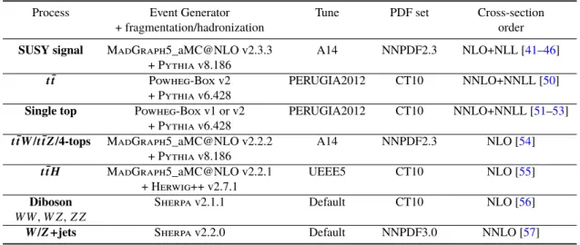
Monte Carlo (MC) samples of simulated events are used to model the signal and to aid in the estimation of SM background processes, except multijet processes which are estimated

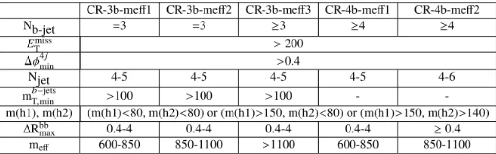
For the dominant t t ¯ , single-top, and Z +jets backgrounds, the expected yield in the SRs is estimated by scaling each MC prediction by a normalization factor (NF) derived from

The cross-sections used to normalise the MC samples are varied according to the uncertainty in the cross- section calculation, which is 13% for t¯ tW , 12% for t¯ t Z production

For hadronic tau lepton decays selected by offline algorithms, the correction factor on the tau trigger identification efficiency is measured with a relative precision of 3–8% for p

Simulated event samples are used to model the signal and background processes in this analysis, except multijet processes which are estimated from data.. These samples are interfaced

The observed and expected upper limits at 95% confidence level (CL) on the number of events from BSM phenomena for each signal region (S 95 obs and S 95 exp ) are derived using the CL