ATLAS-CONF-2017-029 01May2017
ATLAS CONF Note
ATLAS-CONF-2017-029
1st May 2017
Measurement of the tau lepton reconstruction and identification performance in the ATLAS
experiment using p p collisions at √
s = 13 TeV
The ATLAS Collaboration
This document details measurements of the performance of the reconstruction and identific- ation of hadronic tau lepton decays using the ATLAS detector. The performance of these algorithms is measured withZboson or top quark decays to tau leptons and uses the full 2015 dataset ofppcollisions collected at the LHC, corresponding to an integrated luminosity of 3.2 fb−1and a centre-of-mass energy
√
s=13 TeV. The measurements include the perform- ance of the identification, trigger, energy calibration, and electron discrimination algorithms for reconstructed tau candidates. The simulation to data correction factor on the offline tau identification efficiency is measured with a relative precision of 5% (6%) for one (three) track reconstructed tau candidates. For hadronic tau lepton decays selected by offline algorithms, the correction factor on the tau trigger identification efficiency is measured with a relative precision of 3–8% for pT(τhad) < 100 GeV and 8–14% for 100 < pT(τhad) < 300 GeV, depending on the transverse energy and the number of associated tracks. The correction factor on the tau energy scale is measured with a relative precision of 2% (3%) for one (three) track reconstructed tau candidates. The correction factor on the probability of misidentifying an electron as a hadronic tau lepton decay is measured with a relative precision of between 3–14%, depending on the pseudorapidity of the reconstructed tau candidate.
© 2017 CERN for the benefit of the ATLAS Collaboration.
Reproduction of this article or parts of it is allowed as specified in the CC-BY-4.0 license.
Contents
1 Introduction 3
2 ATLAS detector 4
3 Data and simulation samples 4
4 Object selection 5
5 Reconstruction, energy calibration and identification of hadronic tau decays 6
5.1 Tau reconstruction 6
5.2 Tau energy calibration 7
5.3 Tau identification 8
5.4 Electron discrimination 10
5.5 Tau trigger identification 10
6 Z →τµτhadtag–and–probe analyses 11
6.1 Common event selection 11
6.2 Offline tau identification efficiency measurement 13
6.2.1 Signal and background estimation 13
6.2.2 Results 15
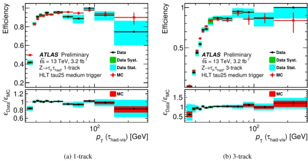
6.3 Trigger efficiency measurement 20
6.3.1 Signal and background estimation 20
6.3.2 Results 20
6.4 Offlineτhad−visin-situ energy scale measurement 23
6.4.1 Energy scale extraction 23
6.4.2 Results 24
7 t¯ttag-and-probe trigger efficiency measurement 25
7.1 Event selection 25
7.2 Signal and background processes 25
7.3 Results 26
8 Z → eetag-and-probe analysis 28
8.1 Event selection 28
8.2 Signal and background processes 28
8.3 Results 29
9 Summary and conclusions 30
Appendix 35
A Tau Identification input variables ofZ →τµτhadtag-and-probe analysis 35
1 Introduction
With a mass of 1.777 GeV and a proper decay length of 87µm [1], tau leptons decay either leptonically (τ→`ν`ντ,`=e, µ) or hadronically (τ→hadronsντ, labelled asτhad) and do so typically before reaching active regions of the ATLAS detector. In this note, only hadronic tau lepton decays are considered. The hadronic tau lepton decays represent 65% of all possible decay modes. The hadronic decay products contain one or three charged pions in 72% and 22% of all cases, respectively. In 68% of all hadronic decays, at least one associated neutral pion is also produced. The neutral and charged hadrons stemming from the tau lepton decay make up the visible part of the tau lepton, and in the following are referred to asτhad−vis.
The main background to hadronic tau lepton decays is from jets of energetic hadrons produced via the fragmentation of quarks and gluons; Both are present at trigger level (also referred to asonlinein the following) as well as during the event reconstruction (referred to asoffline). Discriminating variables based on the narrow shower in the calorimeter, the distinct number of tracks and the displaced tau lepton decay vertex are used to distinguishτhad−viscandidates from jets. Electrons also form an important background for τhad−vis containing one charged hadron. Therefore a specific method to suppress this background is devised too.
Final states with hadronic tau lepton decays are an important part of the ATLAS physics program. This places strong requirements on bothτhad−vis reconstruction and identification algorithms, as well as the performance measurements of the algorithms. The algorithms involved in triggering, reconstructing and identifying tau leptons during proton-proton collisions with a centre-of-mass energy
√
s = 8 TeV are described in Ref. [2], and the updates to these algorithms for
√
s = 13 TeV data collected in 2015 are described in Ref. [3].
This note first gives an overview of the tau reconstruction, energy calibration and identification algorithms and describes further updates to these algorithms for 2016 data-taking. The performance measurements of the triggering, energy calibration and identification algorithms using the 2015 data are described in the remaining sections. The performance of online and offline tau identification, and the tau energy scale calibration are measured using atag-and-probemethod applied to events enriched in the Z →ττ process, with one tau lepton decaying to muon and neutrinos,τµ(tag), and the other decaying to hadrons and neutrino, τhad (probe). The performance of the online and offline tau identification algorithms in simulation and in recorded data are measured and correction factors are derived. For the tau energy scale measurement, the reconstructed visible mass distribution of the muon andτhad−vissystem is determined in both data and simulation, and the energy calibration required to obtain agreement is calculated.
In order to extend the range of the pT spectrum of tau candidates, the performance of the online tau identification algorithm is also measured using events enriched in the t¯t process. This measurement similarly uses the tag-and-probe method with a muon (tag) and a hadronic tau lepton decay (probe).
Finally, the performance of the electron rejection algorithm is measured. The tag-and-probe method is used in events enriched inZ →eedecays featuring at least one electron (tag) and a tau candidate (probe), and the efficiency of the electron rejection algorithm is measured and correction factors are derived.
This note is organised as follows. After a description of the ATLAS detector in section2, the data and simulation samples used in the studies presented are described in section 3. The reconstruction and requirements on the objects used in this note are described in section 4, with the tau reconstruction, energy calibration, identification, electron discrimination and trigger algorithms described separately in more detail in section5. The tau identification, trigger and energy scale performance measurements using
the tag-and-probe method in Z → τµτhad events are described in section6. Similarly the tag-and-probe studies carried out usingt¯tand Z →eeevents are described in sections7and8respectively. Finally, a summary of the measurements is given and their use in physics analyses detailed.
2 ATLAS detector
The ATLAS detector [4] consists of an inner tracking system surrounded by a superconducting solenoid, electromagnetic (EM) and hadronic (HAD) calorimeters, and a muon spectrometer (MS).
The inner detector is immersed in a 2 T axial magnetic field, and consists of silicon pixel and microstrip (SCT) detectors inside a transition radiation tracker (TRT), providing charged particle tracking in the region|η| <2.51. For the√
s= 13 TeV run, a fourth layer of the pixel detector, the InsertableB-Layer (IBL) [5], has been inserted at an average radius of 33.2 mm, providing an additional position measurement with 8µm resolution in the(x,y)plane and 40µm alongz.
The EM calorimeter uses lead and liquid argon (LAr) as absorber and active materials, respectively. In the central rapidity region, the EM calorimeter is divided in three layers, one of them segmented in thin ηstrips for optimalγ/π0separation, completed by a presampler layer for|η| < 1.8. Hadron calorimetry is based on different detector technologies, with scintillator tiles (|η| < 1.7) or LAr (1.5 < |η| < 4.9) as active media, and uses steel, copper, or tungsten as the absorber material. The calorimeters provide coverage within |η| < 4.9. The MS consists of superconducting air-core toroids, a system of trigger chambers covering the range|η| <2.4, and high-precision tracking chambers allowing muon momentum measurements within|η|< 2.7.
The ATLAS trigger system consists of two levels which reduce the initial bunch crossing rate to a manageable rate for disk storage while keeping interesting physics events. The first level (L1) is hardware- based and uses a subset of the detector information to reduce the accepted event rate to 100 kHz [6].
This is followed by a software-based High Level Trigger (HLT) that further reduces the average recorded collision rate to around 1 kHz.
3 Data and simulation samples
The data used in this note were recorded by the ATLAS experiment during the 2015 LHC run with proton-proton collisions at a centre-of-mass energy of
√s = 13 TeV. They correspond to an integrated luminosity of 3.2 fb−1. To ensure good data quality, the inner-detector tracking systems, calorimeters and muon spectrometer are required to be fully operational.
The simulated background processes consist of the production of Z+jets,W+jets, single top quarks and tt¯pairs. They are modelled with several event generators as described below, while contributions from multi-jet production are estimated with data-driven techniques as described in each section.
1ATLAS uses a right-handed coordinate system with its origin at the nominal interaction point (IP) in the centre of the detector and thez-axis along the beam direction. Thex-axis points from the IP to the centre of the LHC ring, and they-axis points upward. Cylindrical coordinates(r, φ)are used in the transverse(x,y)plane,φbeing the azimuthal angle around the beam direction. The pseudorapidity is defined in terms of the polar angleθasη=−ln tan(θ/2). The distance∆Rin theη−φspace is defined as∆R=q
(∆η)2+(∆φ)2.
Simulated samples ofZ+jets events andW+jets events are produced usingPOWHEG-BOX v2[7–9] inter- faced toPYTHIA 8.186[10] with the AZNLO tune [11]. In this sample,PHOTOS++ v3.52 [12,13] is used for photon radiation from electroweak vertices and charged leptons. AllW/Z+jets samples use the CT10 PDF set and are normalised to the next-to-next-to-leading-order (NNLO) cross sections calculated usingFEWZ[14,15].
ThePOWHEG-BOX v2program with the CT10 PDF set is used for the generation oft¯t pairs and single top quarks in theW t- ands-channels. Samples oft-channel single-top-quark events are produced with thePOWHEG-BOX v1 [7, 8] generator employing the four-flavour scheme for the NLO matrix element calculations together with the fixed four-flavour scheme PDF set CT10f4; the top-quark decay is simulated withMadSpin [16]. For all samples of top-quark production, the spin correlations are preserved and the parton shower, fragmentation and underlying event are simulated usingPYTHIA 6.428 [17] with the CTQ6L1 PDF set and the corresponding Perugia 2012 tune [18]. Photon radiation from charged leptons and electroweak vertices is simulated usingPHOTOS++ v3.52. The top-quark mass is set to 172.5 GeV.
Thet¯tproduction sample is normalised to the NNLO cross section, including soft-gluon resummation to next-to-next-to-leading-logarithm accuracy (Ref. [19] and references therein). The normalisation of the single top quark event samples uses an approximate NNLO calculation from Refs. [20–22].
The effect of multiple proton (pp) interactions, referred to as pile-up, is simulated by overlaying minimum- bias interactions on the generated events. The simulated events are reweighted such that the average number ofppinteractions per bunch crossing has the same distribution in data and simulation.
4 Object selection
Muons are reconstructed by combining an inner detector track with a track from the MS [23], and must lie within|η| < 2.5, with a transverse momentum requirement of pT > 10 GeV for the Z → eeanalysis and pT > 7 GeV for all other analyses. Corrections to simulated reconstruction efficiencies, derived from the data, are applied to the simulated samples. The muon candidates have to pass a “loose” muon identification requirement, which corresponds to a 98% efficiency.
Electrons are reconstructed by matching clustered energy deposits in the electromagnetic calorimeter to tracks reconstructed in the inner detector, and are required to have pT > 15 GeV and |η| < 2.47 (excluding the transition region between the barrel and end-cap calorimeters, corresponding to the region 1.37 < |η| < 1.52). Electrons are identified using the signal and background probability density functions for several discriminating variables detailed in Ref. [24,25]. A likelihood (LLH) function is constructed with several working points available, corresponding to cuts on the likelihood score with different levels of signal efficiency and background rejection. For the studies in this document, themediumidentification working point is required to select electron candidates and thevery looseworking point is used for vetoing electrons faking taus. Corrections to the reconstruction and identification efficiencies derived from the data are applied to the simulated samples.
For muons and electrons, the scalar sum of the transverse momenta of tracks within a cone ofpT-dependent size,∆R <min (10 GeV/pT,0.3), centred on the lepton candidate track and excluding the lepton track, is required to be less than apT-dependent fraction of the lepton transverse momentum. Additionally, the sum of the calorimeter energy deposits in a cone of size∆R < 0.2 around the lepton, excluding energy associated with the lepton candidate, must be less than apT dependent percentage of the lepton energy.
This requirement, referred to asgradient isolation, is used in the electron rejection and trigger efficiency measurements, and has a 90 (99)% efficiency at 25 (60) GeV.
Another isolation criterion uses a similar definition, except with a fixed cone size of∆R < 0.4 for tracks and with the threshold values fixed at 1% and 4% for the sum of track momenta, and the sum of the calorimeter energy deposits respectively. This isolation, referred to asfixed-thresholdisolation, provides a stronger multi-jet rejection. Fixed-threshold isolation is used to select electrons and muons in the offline tau identification and tau energy scale measurements.
Jets are constructed using the anti-kt algorithm [26], with a distance parameter R = 0.4. Three- dimensional clusters of calorimeter cells called TopoClusters [27], calibrated using a local hadronic calibration (LC) [28], serve as inputs to the jet algorithm. Jets are required to be within |η| < 4.5. A dedicatedb-tagging algorithm described in Ref. [29,30] is used to identify jets associated with the decay of ab-quark in the range|η| <2.5, and has a 77% efficiency.
The reconstruction, energy calibration and identification of the hadronic decays of tau leptons are described in the next section whilst the geometric overlap of objects with∆R<0.2 is resolved by selecting only one of the overlapping objects in the following order of priority: muons, electrons, τhad−vis candidates, and jets. The missing transverse momentum, with magnitudeEmiss
T , is calculated from the vector sum of the transverse momenta of all reconstructed electrons, muons,τhad−visand jets in the event, as well as a term for the remaining tracks [31].
5 Reconstruction, energy calibration and identification of hadronic tau decays
This section gives an overview of the online and offline algorithms used in the reconstruction, energy calibration and identification of the hadronic decays of tau leptons. A detailed description of the offline algorithms used in the reconstruction, baseline energy calibration and identification of hadronic tau decays during the 2015 data-taking period of Run 2, as well as the expected performance of the reconstruction algorithms and associated systematic uncertainties can be found in Ref. [3].
5.1 Tau reconstruction
Tau candidates are seeded by jets formed using the procedure described in Section4. Jets seeding tau candidates are additionally required to havepT > 10 GeV and|η| < 2.5. Tau candidates in the transition region between the barrel and forward calorimeters, 1.37 < |η| < 1.52, are vetoed.
A tau vertex is chosen as the candidate track vertex with the largest fraction of momentum from tracks associated (∆R< 0.2) with the jet. The tracks must pass requirements on the number of hits in the tracker and have pT > 1 GeV. Additional requirements are placed on the shortest distance from the track to the tau vertex in the transverse plane,|d0| < 1 mm, and the shortest distance in the longitudinal plane,
|∆z0sin(θ)| < 1.5 mm where θ is the polar angle of the track and z0 is the point of closest approach along the longitudinal axis. Provided these requirements are passed the tracks are then associated tocore (0<∆R<0.2) andisolation(0.2< ∆R<0.4) regions around the tau candidate.
The direction (eta/phi) of the tau candidate is calculated using the vectorial sum of the TopoClusters within
∆R < 0.2 of the seed jet barycenter, using the tau vertex as the origin. The mass of the tau candidate
is defined to be zero and consequently the transverse momentum,pT, and the transverse energy, ET are identical. The energy of the tau is obtained through dedicated calibration schemes, described in the following section.
5.2 Tau energy calibration
A tau-specific energy calibration is applied to the tau candidate in order to correct the energy deposition measured in the detector to the average value of the energy carried by the measured decay products at the generator level. Two calibrations are available, known as the baseline calibration, and the boosted regression tree (BRT) based calibration. With the exception of the BRT-specific tau energy scale meas- urement presented in section6.4, all measurements performed in this note use the baseline calibrated tau candidates.
The baseline correction to the tau energy is calculated as:
Ecalib = ELC−Epileup R
ELC−Epileup,|η|,np . (1)
First, a correction to the LC-calibrated sum of the energy of all TopoClusters within∆R< 0.2 of the tau candidate,ELC, is applied for the energy contribution,Epile−up, from multiple interactions occurring in the same bunch crossing (referred to as pileup). It is found thatEpile−upincreases linearly with the number of primary verticesNPV. Thus, the pile-up correction is derived as:
Epileup(NPV,|η|,np)= A(|η|,np)×(NPV− hNPVi), (2) and calculated separately for 1-track and 3-track tau candidates, denoted by np. Following the Run 1 convention, the pile-up correction, A(|η|,np)×(NPV− hNPVi), vanishes for a value ofNPV equal to the average pile-up conditions of the MC samples, e.g. NPV≈ 14. The linear coefficient Ais extracted from a linear fit of ELC from simulated samples as a function of (NPV− hNPVi) in bins of |η|. The detector response calibration,R, extracted as the Gaussian mean of the
ELC−Epileup /Evis
truedistribution, is then applied. Here,Evis
trueis the energy of the generated tau decay products, including final state radiation, but excluding the contribution of the neutrinos
The energy resolution of the baseline method is excellent at high pT but quickly degrades at low pT. A method of reconstructing the individual charged and neutral hadrons in tau decays has recently been developed by the ATLAS experiment and is known as "Tau Particle Flow" (TPF) [32]. The method significantly improves the tau energy resolution at lowpTdue to the superior measurement of the charged pion momentum from the tracking system. An improved energy calibration has therefore been introduced which combines the information from the baseline and TPF methods together with additional calorimeter and tracking information via a multivariate-analysis technique. This technique is referred to as a BRT method, and is implemented using the TMVA package [33].
To train the BRT, tau candidates satisfying the medium tau identification requirement, which is described in Section5.3, coming from simulated Z/γ∗ → ττ events are used. The two figures of merit, used to determine which input variables and BRT tuning parameters are optimal, are defined as follows: the resolutionis defined as half of the 68% central interval of the ratio of the calibratedτhad−vis transverse momentum to the generatedτhad−vistransverse momentum,ptrue,vis
T , whilst thenon-closureis the offset of the most probable value of that ratio from unity. The most probable value is used instead of the arithmetic
mean in this case to reduce the impact of the asymmetric tails of the distribution. The transverse component of the sum of the momenta of the reconstructed charged hadron and neutral pion constituents is referred to aspTPF
T , and the transverse momentum at LC-scale ispLC
T . As the resolution ofpTPF
T is better thanpLC
T
at low pT, and vice-versa at higher pT, the interpolated transverse momentum, pinterp
T , is defined in the following equation:
pinterp
T = fx×pLC
T +(1− fx)×pTPF
T , (3)
where fxis a weight between zero and one and is a function ofpLC
T : fx(pLC
T ) = 1 2
* ,
1+tanh pLC
T −xGeV 20 GeV
+ -
. (4)
The symbol x defines the point where the transition from low pT to high pT occurs, and is chosen to be x = 250. The regression target of the BRT training is the ratio of the generated τhad−vis transverse momentum topinterp
T .
The final input variables used in the BRT are listed and described in Table1. The transverse momentapLC
T
andpTPF
T provide basic knowledge about theτhad−visenergy. The BRT is less powerful when two variables are highly correlated and so to reduce the correlation, ratios of these variablespLC
T /pinterp
T andpTPF
T /pinterp
T
are used instead of the raw values.
The moments of the individual TopoCluster constituents of the tau candidates, such asλcentre, Dλ2E
,hρi, fpresampler, andPEM, used in the LC calibration as described in Ref. [28], are found to be powerful inputs to the BRT-based tau energy calibration. In order to simplify the use of these variables, they are re-defined at the per-tau level, as the energy-weighted average of these moments for all constituent TopoClusters.
The variablesµandnPVare included to provide information about multiple interactions occurring in the same bunch crossing, whilstγπ andnπ0are variables that provide information about the decay modes of the tau candidate and improve the resolution at lowpT.
Figure1shows the τhad−visenergy resolution of baseline, TPF-based and BRT-based calibrations. In the region pT < 100 GeV, the BRT-based tau energy calibration improves on the baseline resolution by a factor of two, while at highpTthe performance is comparable.
5.3 Tau identification
The tau identification algorithm is designed to reject backgrounds from quark- and gluon-initiated jets.
The identification uses Boosted Decision Tree (BDT) based methods [34,35]. As described in Ref. [3], the BDT for tau candidates associated with one and three tracks are trained separately with simulated Z/γ∗→ττfor signal and dijet events (selected from data) for background. Three working points labelled loose,mediumandtightare provided, and correspond to different tau identification efficiency values, with the efficiency designed to be independent of pT. The target efficiencies are 0.6, 0.55 and 0.45 for the generated 1-track loose, medium and tight working points, and 0.5, 0.4 and 0.3 for the corresponding generated 3-track target efficiencies. The input variables to the BDT are corrected such that the mean of their distribution for signal samples is constant as a function of pile-up. This ensures that the efficiency for each working point does not depend strongly on the pile-up conditions. The figures of all the input variables can be found in AppendixA
Number of primary vertices,nPV Number of primary vertices in the event.
Average interactions per crossing,µ
Average number of interactions per bunch crossing.
Cluster shower depth,λcentre
Distance of the cluster shower centre from the calorimeter front face measured along the shower axis.
Cluster second moment inλ,D λ2E
Second moment of the distance of a cell,λ, from the shower centre along the shower axis.
Cluster first moment in energy density,hρi
Cluster first moment in energy densityρ=E/V, whereEandVrepresent the energy and volume of the cluster, respectively.
Cluster presampler fraction, fpresampler
Fraction of cluster energy deposited in the barrel and endcap presamplers.
Cluster EM-like probability,PEM
Classification probability of the cluster to be EM-like, as described in Ref. [28].
Number of associated tracks,ntrack
Number of tracks associated with theτhad−vis. Number of reconstructed neutral pions,nπ0
Number of reconstructed neutral pions associated with theτhad−vis. Relative difference of pion energies,γπ
Relative difference of the total charged pion energy, Echarged, and the total neutral pion energy,Eneutral: γπ =(Echarged−Eneutral)/(Echarged+Eneutral).
Calorimeter-based pseudorapidity,ηcalo Calorimeter-based (baseline) pseudorapidity.
Interpolated transverse momentum, pinterp
T
Transverse momentum interpolated from calorimetric corrections to energy meas- urement and TPF reconstruction.
Ratio of pLC
T topinterp
T , pLC
T /pinterp
T
Ratio of the local hadron calibration transverse momentum topinterp
T .
Ratio of pTPF
T topinterp
T , pTPF
T /pinterp
T
Ratio of the TPF reconstruction transverse momentum,pTPF
T , topinterp
T .
Table 1: List of input variables used in the boosted regression tree for τhad−vis energy calibration. The cluster variables are defined as the energy-weighted average of the moments for all constituents TopoClusters, as described in detail in Ref. [28].
) [GeV]
had-vis
(τ pT
50 100 150 200 250
) resolution [%]had-visτ ( Tp
5 10 15 20
Baseline BRT ATLAS Preliminary Simulation
Figure 1: The resolution of the baseline and the BRT-basedτhad−visenergy calibration. The resolution, shown as a function of the generated taupT, is defined as half of the 68% central intervals of the ratio of the calibratedpTto the true visiblepT.
5.4 Electron discrimination
In order to reduce the electron background, reconstructed tau candidates associated with a single track and within a distance of∆R < 0.4 of a reconstructed electron are rejected if the electron passes avery looseworking point of the electron likelihood identification algorithm, as mentioned in Section4. This electron likelihood score cut is tuned to yield a 95% efficiency for hadronically decaying taus, and the cut on the electron identification likelihood score is dependent on thepTand|η|of the tau candidate. The cut value on the electron identification likelihood has been updated in comparison to Ref. [3] to reflect the 2015 data-taking conditions [25].
5.5 Tau trigger identification
Due to the technical limitations of the ATLAS trigger system [36], the online reconstruction of hadronic tau lepton decays is modified compared to the offline reconstruction. At L1, trigger towers are defined in the EM and hadronic calorimeters with a granularity of∆η×∆φ= 0.1×0.1. A core region is made up of a set of 2×2 trigger towers and a requirement is placed on the transverse energy sum of the two most energetic adjacent EM calorimeter towers. A requirement can also be placed on the transverse energy deposited in an isolation region of calorimeter towers around the core.
At HLT, the energy is recalculated using LC-calibrated TopoClusters of calorimeter cells contained in a
∆R=0.2 cone around the L1 tau direction. The energy is calibrated using the baseline method described in Section5.2, using dedicated factors derived to account for the different LC calibration constants and pile-up correction scheme used at trigger level. Additionally, the pile-up subtraction term in the baseline calibration is calculated using the average number of interactions per crossing instead of the number of primary vertices, as the latter is not available at trigger level. A minimum transverse energy requirement is placed on the online tau candidate.
A multi-stage tracking algorithm is then used to reconstruct tracks in a sufficiently large∆Rcone around the tau candidate. The first stage, referred to as fast-tracking, reconstructs tracks using trigger-specific
pattern recognition algorithms in two steps. In the first step the highest-pT track is identified in a narrow cone (∆R <0.1) around the tau direction and along the direction of the beam in the range|z| <255 mm.
The second step reruns the fast-tracking software in an extended cone (∆R<0.4) around the tau direction but with the tracks required to emanate from the same position along the beamline as the leading track.
A requirement is made on the number of tracks within a core (∆R<0.2) and isolation (0.2 <∆R <0.4) region of 0< Ntracks
core < 4 and Ntracks
iso < 2, respectively. Finally, the detector hits and tracks identified in the fast-tracking stages are used as seeds in an HLT-tracking stage. HLT-tracking refers to the precision reconstruction of tracks with algorithms similar to those used in the offline reconstruction.
The HLT precision track and calorimeter information is used to calculate a number of pileup corrected variables which are then input into an online tau BDT. The variables used in the online BDT are the same as those used in the offline BDT, with the exception that the lifetime variables are calculated with respect to the beamspot instead of the tau vertex, as full event vertex reconstruction is not available at the HLT. The offline BDT training is used directly at trigger level, as it was found to provide good rejection while minimizing the orthogonality between the trigger and offline selection. As in the case of offline tau identification, three identification working points are available for online tau candidates with one or three associated tracks: loose, medium and tight. These working points were tuned to provide target efficiencies of approximately 0.95 (0.70) after their offline counterpart identification is applied for taus with one (three) associated tracks
6 Z → τ
µτ
hadtag–and–probe analyses
In this section, the performance of the identification, trigger and energy reconstruction algorithms are evaluated with a data sample enriched inZ →τµτhadevents where one tau lepton decays to a muon and the other decays hadronically, with associated neutrinos. The chosen tag-and-probe approach consists of selecting events triggered by the presence of a muon (tag) and containing a hadronically decaying tau lepton candidate (probe) in the final state and studying the performance of the identification, trigger and energy reconstruction algorithms. In this sectionsignalrefers to aτhad−vis candidate geometrically matched with a generatedτhad−visor theZ →τµτhad event containing such tau candidates.
6.1 Common event selection
To select Z → τµτhad events, a single-muon trigger with the threshold of pT > 20 GeV is used. The offline reconstructed muon candidate must havepT >22 GeV and be geometrically matched to the online muon. Events are required to have no additional electrons or muons and at least one τhad−vis candidate with 1 or 3 tracks. If there are multipleτhad−viscandidates, only the leadingpTcandidate is considered. In addition, a very loose requirement on the tau identification BDT output (>0.3) is made which suppresses jets while being more than 99% efficient for the generatedτhad−vis. The muon andτhad−viscandidates are required to have opposite-sign electric charges (OS). Events withb-tagged jets are rejected, after which the contribution from top quark backgrounds is reduced from 1-3% to 0.3-0.8%, depending on the analysis and the number of charged tracks associated to the tau candidate. The associatedb-tagging systematic uncertainty is found to be negligible, since the probability of passing theb-jet veto is very high (> 99%) for jets that do not originate from ab-quark.
A series of selection requirements is used to suppressW+ jets (mainlyW → µνµ) events. The transverse mass of the muon and Emiss
T system, mT = q 2pµ
T·Emiss
T (1−cos∆φ(µ,Emiss
T )), is required to be less than 50 GeV, wherepµ
T is the transverse momentum of the muon, and∆φ(µ,Emiss
T )is the∆φseparation between the muon and the missing transverse momentum. The quantityΣcos∆φ = cos∆φ(µ,Emiss
T )+ cos∆φ(τhad−vis,Emiss
T )is required to be greater than−0.5, where∆φ(τhad−vis,Emiss
T )is the∆φseparation between theτhad−visand the missing transverse momentum.
In addition to the above common selection, the medium offline tau identification requirement is applied in the energy scale measurement. Several offline working points, i.e. loose, medium and tight, are applied in the online tau identification efficiency to derive the corresponding trigger efficiencies. A requirement on the invariant mass of the muon and tau candidate, 45 GeV< mvis(µ, τhad−vis) < 80 GeV, is applied in both online and offline tau identification efficiency measurements, but not in the energy scale measurement since the mvis(µ, τhad−vis) distribution is used to constrain the tau energy scale. To reduce the large contamination from misidentified jets in the offline tau identification efficiency measurement, in which the medium tau identification requirement is not applied, the lower threshold onΣcos∆φis tightened to−0.1.
The detailed event selections and the signal purity, i.e. the estimated fraction of generated tau leptons to the total predicted number of events after applying the signal selection requirements listed above, are summarised in Table2.
Analyses Offline Identification Online Identification TES
mT <50 GeV <50 GeV <50 GeV
Σcos∆φ >−0.1 > −0.5 >−0.5
mvis (45–80 GeV) (45–80 GeV) –
Tau Identification – various medium
Purity 20% (before ID) 73% (medium) 65%
Table 2: Summary of theZ→τµτhadevent selections and purities in the online and offline tau identification, as well as the tau energy scale measurement.
After the final selection, besides a small fraction of muons misidentified as hadronic tau lepton decays (which are modelled via simulation), the main background for the probe τhad−vis candidates are jets misidentified as hadronic tau lepton decays fromW+jets and multi-jet events. In these jet to τ fake events, especially multi-jet events, the correlation of the charge sign between misidentified jets and the muon is not as strong as in the case ofZ → τµτhad signal events. Therefore, the events with same sign (SS) charge are used to model the jet to τ fake background. Due to the residual charge correlation, there are more background events with opposite sign charge than with same sign. To take this charge correlation into account, a normalisation factor on multi-jet events is measured from the multi-jet control region, defined below, by comparing events with opposite sign charge and same sign charge. For the W+jets events, the trigger and energy scale measurements use simulated events to model the difference between opposite sign events and same sign events, the so called ‘OS–SS’ method, with the correction factors derived fromW+jets control region events with opposite sign charge and the same sign charge requirements, respectively. The offline identification measurement follows the same principle but takes a slightly different approach, as discussed in section6.2.1.
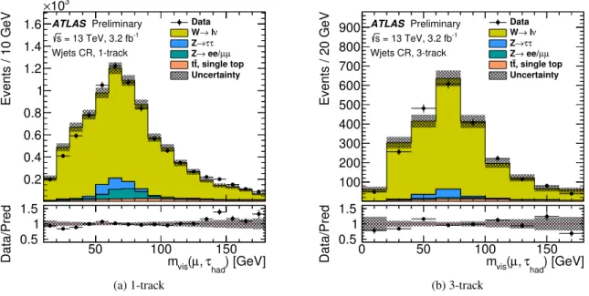
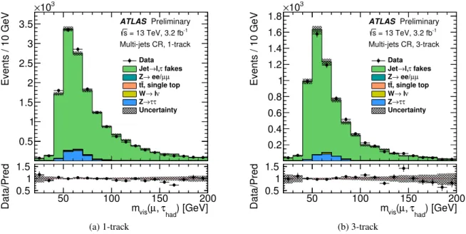
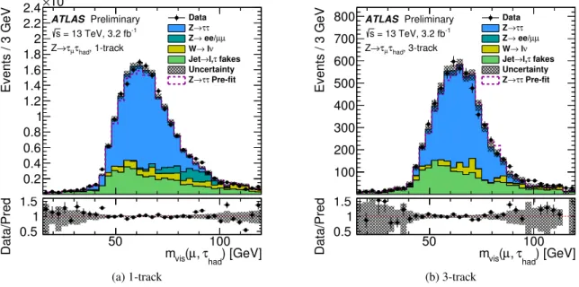
To improve the modelling of the jet background, two control regions enriched in specific background processes are used. AW+jets control region, as shown in Figure2, is selected by requiringEmiss
T > 30 GeV andmT >60 GeV, and a multi-jet control region, as shown in Figure3, is selected by inverting the muon
isolation requirement. The identification is applied in the control regions for the energy scale and the trigger measurements, while the offline identification measurement has the control regions both with and without the tau identification requirement, in order to extract the yield in both cases.
Events / 10 GeV
0.2 0.4 0.6 0.8 1 1.2 1.4 1.6
103
×
ATLAS Preliminary = 13 TeV, 3.2 fb-1
s
Wjets CR, 1-track
Data lν W→
τ τ Z→
µ ee/µ Z→
, single top t
t
Uncertainty
) [GeV]
τhad
, (µ mvis
50 100 150
Data/Pred
0.5 1 1.5
(a) 1-track
Events / 20 GeV
100 200 300 400 500 600 700 800
900 ATLAS Preliminary = 13 TeV, 3.2 fb-1
s
Wjets CR, 3-track
Data lν W→
τ τ Z→
µ ee/µ Z→
, single top t
t
Uncertainty
) [GeV]
τhad
, (µ mvis
0 50 100 150
Data/Pred
0.5 1 1.5
(b) 3-track
Figure 2: The distribution ofmvis, the invariant mass of theτhad−visand muon system, in theW+jet control region.
The tau candidate is required to pass medium identification. The error band contains only the statistical uncertainty.
6.2 Offline tau identification efficiency measurement
In the offline tau identification efficiency measurement, the contamination from jet backgrounds before the application of the tau identification poses the greatest challenge. To estimate the background contamination in data, a template fit is performed using a variable with high separation between signal and background, to estimate the normalisation factors for both signal and background. The signal contribution to data before the application of the tau identification requirement is estimated directly from the fit, whilst the signal contribution to data after the application of the various tau identification working points is extracted by subtracting the estimated backgrounds from the data, after applying the same background normalisation factors as those before the identification is applied.
The variable used is the track multiplicity, defined as the sum of the number of core (∆R<0.2) and outer (0.2<∆R<0.6) tracks associated to theτhad−viscandidate. Outer tracks are only considered if they fulfil the track separation requirement,Douter=min([pcore
T /pouter
T ]·∆R(core,outer)) <4, wherepcore
T refers to any track in the core region, and∆R(core,outer)refers to the distance between the candidate outer track and any track in the core region. More details can be found in Section 4 of Ref. [2].
6.2.1 Signal and background estimation
This section describes how the templates for the signal and the background are constructed and how the tau identification efficiency is measured. The tau candidate track multiplicity distribution of signal events
Events / 10 GeV
0.5 1 1.5 2 2.5 3 3.5
103
×
ATLAS Preliminary = 13 TeV, 3.2 fb-1
s
Multi-jets CR, 1-track Data
fakes l,τ Jet→
µ ee/µ Z→
, single top t
t lν W→
τ τ Z→ Uncertainty
) [GeV]
τhad
, (µ mvis
50 100 150 200
Data/Pred
0.5 1 1.5
(a) 1-track
Events / 10 GeV
0.2 0.4 0.6 0.8 1 1.2 1.4 1.6 1.8
103
×
ATLAS Preliminary = 13 TeV, 3.2 fb-1
s
Multi-jets CR, 3-track Data
fakes l,τ Jet→
µ ee/µ Z→
, single top t
t lν W→
τ τ Z→ Uncertainty
) [GeV]
τhad
, (µ mvis
50 100 150 200
Data/Pred
0.5 1 1.5
(b) 3-track
Figure 3: The distribution ofmvis, the invariant mass of theτhad−visand muon system, in the multi-jet control region.
The tau candidate is required to pass medium identification. The error band contains only the statistical uncertainty.
is modelled using simulated Z → τµτhad events with a small contribution from t¯t events. Two signal templates are obtained by requiring exactly one or three tracks reconstructed in the core region of the τhad−vis candidate. To improve the fit stability, a combined template is used to model both the one track τhad−visand the three trackτhad−vis which are shown in separated colors in Figure4. A single template is used to model the background from quark- and gluon-initiated jets that are misidentified as hadronic tau lepton decays:
FOSbkg =rQC D ·
FSSdat a−FSSW+jet s C R ·TSSW+jet s MC
+FOSW+jet s C R·TOSW+jet s MC, (5) whereF terms represent the template in data and theW+ jets control region for OS and SS, andT terms represent transfer factors, which are measured as the ratio of the simulated events with the signal region selection to simulated events with theW+jets control region selection for the OS and SS requirements, as a function of the track multiplicity. The background is mainly composed of multi-jet andW+jets events with a minor contribution from Z+jets events. Jet to tau fakes in t¯t events is included in the analysis and covered together asW+ jets. The jet template is constructed starting with data events in the same sign control region
FSSdat a
, a region enriched in events with jets misidentified as tau candidates. The contributions fromW+jets andZ+jets in the SS control region
FSSW+jet s C R ·TSSW+jet s MC
are subtracted to yield the multi-jet only contribution. Then, to correct for the difference in normalisation between the same sign multi-jet events and the opposite sign ones, the template is scaled by the ratio
rQC D of OS/SS multi-jet events. To reduce the Z → ττ signal contamination in the multi-jet control region, events with 45 GeV < mvis(`, τhad−vis) < 80 GeV in the multi-jet control region are rejected. Finally, the OS contributions fromW+jets events are added to complete the template. The shape of theW+jets contribution is estimated from theW+jets control region
FOSW+jet s C R
and normalised to the signal region using transfer factors
TOSW+jet s MC
derived using simulatedW+jets events. The jet templates both with and without the identification requirements are built with this procedure.
An additional background is the contamination due to the misidentification of muons and electrons as tau candidates, and comes mainly fromZ → µµprocesses. This small background contribution is modelled by simulated Z → ee/µµ, t¯t, Z → ττ, diboson events where the reconstructed tau candidate probe is matched to a generated muon or electron. The yield of events where the lepton is misidentified as a tau candidate is typically less than 1% of the total signal yield.
With the normalisation factor of the signal and jet templates allowed to float, the signal plus background model of the track multiplicity is fitted to the data without identification. The normalisation factor of the jet template obtained from this fit is applied to the jet templates both before and after each tau identification working point is applied. The yield of theτsignal both before and after the application of each working point is obtained from the data subtracted by the estimated backgrounds from simulated muons and the jet template with the normalisation factor applied.
The efficiency for a given identification working point is calculated by taking the ratio of the extracted number of signal events before and after the identification criteria is applied.
6.2.2 Results
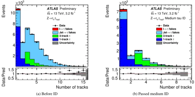
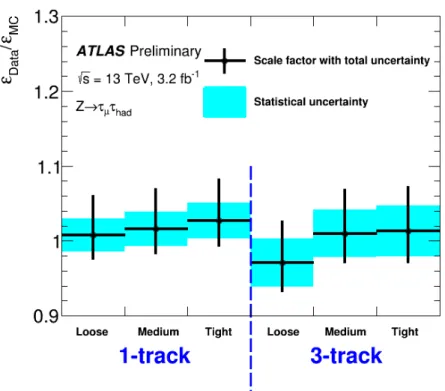
Figure4shows the track multiplicity distributions before and after applying the medium tau identification requirement. To account for the small differences between data and simulation, correction factors (also referred to as scale factors), defined as the ratio of the efficiency in data (εData) to the efficiency in simulation (εMC) forτhad−vissignal to pass a certain level of identification, are derived. The results are shown in Figure5and found to be compatible with unity.
Events
2 4 6 8 10
103
×
ATLAS Preliminary = 13 TeV, 3.2 fb-1
s τhad
τµ
Z→
Data fakes τ l→
fakes τ Jet→ 3-track τ 1-track τ Uncertainty
Number of tracks
5 10 15
Data/Pred
0.5 1 1.5
(a) Before ID
Events
1 2 3 4 5 6 7
103
×
ATLAS Preliminary = 13 TeV, 3.2 fb-1
s
, Medium tau ID τhad
τµ
Z→
Data fakes τ l→
fakes τ Jet→ 3-track τ 1-track τ Uncertainty
Number of tracks
2 4 6 8 10
Data/Pred
0.5 1 1.5
(b) Passed medium ID
Figure 4: Track multiplicity: the sum of the number of core tracks and the outer tracks in 0.2<∆R<0.6 that fulfil the requirementDouter<4, as defined in the text and Ref. [2]. The true tau and ‘Jet→τfakes’ component are fitted to data while ‘lepton (l)→τfakes’ component is fixed to the simulation prediction. The uncertainty band contains only the statistical uncertainty. Note: the track multiplicity included in the fit is up to 15, as shown in (a).
Figure 5: The scale factors (εData/εMC) needed to bring the offline tau identification efficiency in simulation (εMC) to the level observed in data (εData) for one track and three trackτhad−viscandidates withpT>20 GeV. The combined systematic and statistical uncertainties are shown.
The sources of uncertainty on the scale factors are summarised in Table3. The uncertainty on the signal template is estimated by comparing simulated signal generated with different configurations, such as variations on the amount of detector material, and the hadronic interaction model, e.g. QGSP_BIC and FTFP_BERT models [37–40]. These comparisons are used to evaluate the effect of different simulation models on the relative normalisation of the 1-track to 3-track templates which are fixed to the simulated values in the fit. The uncertainty on the jet template accounts for differences between theW+jets shape in the signal and control regions and is derived from comparisons to simulatedW+jets events, as well as the differences between the multi-jet template shape in the opposite sign and same sign region derived by varying the multi-jet control region selections. The uncertainty due to the normalisation of the misidentified muon background is estimated conservatively by varying the normalisation up and down by 50%.
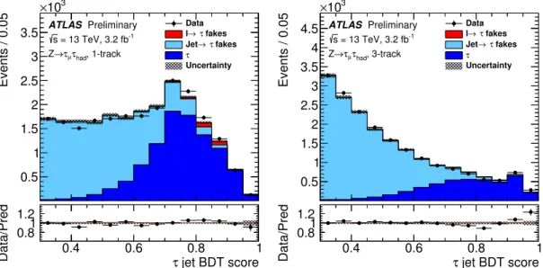
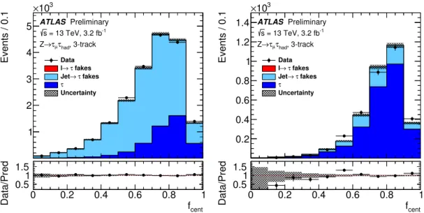
Figure6shows the jet BDT score distribution, while Figures7to10show some of the input variables to the jet discriminant BDT. The figures of all the input variables can be found in AppendixAwhilst the definition of the input variables can be found in Section 5 of Ref. [3]. For both the jet BDT score figure and the input variable figures, the distributions for the signal and background are obtained using the same methods as for the efficiency measurement. Some of the input variables comparisons show discrepancies;
these are globally accounted for by the scale factors derived in the efficiency measurements.
Uncertainty source Uncertainty [%]
1-track 3-track Jet template modelling 1.5 1.5 Tau template modelling 4.4 4.3 Lepton template modelling 1.7 1.7
Statistics 1.7 2.8
Total 5.2 5.6
Table 3: Dominant uncertainties on the tau identification efficiency scale factors estimated with theZboson tag-and- probe method, and the total uncertainty, which combines systematic and statistical uncertainties. These uncertainties apply toτhad−viscandidates passing the medium tau identification algorithm with pT>20 GeV. The uncertainties for other tau identification working points are similar.
Events / 0.05
0.5 1 1.5 2 2.5 3 3.5
103
×
ATLAS Preliminary = 13 TeV, 3.2 fb-1
s
, 1-track τhad
τµ
Z→
Data fakes τ l→
fakes τ Jet→ τ Uncertainty
jet BDT score τ
0.4 0.6 0.8 1
Data/Pred
0.81 1.2
Events / 0.05
0.5 1 1.5 2 2.5 3 3.5 4 4.5
103
×
ATLAS Preliminary = 13 TeV, 3.2 fb-1
s
, 3-track τhad
τµ
Z→
Data fakes τ l→
fakes τ Jet→ τ Uncertainty
jet BDT score τ
0.4 0.6 0.8 1
Data/Pred
0.81 1.2
Figure 6: The jet discriminant BDT output distribution for one track (left) and three track (right)τhad−viscandidates.
The uncertainty band contains only the statistical uncertainty.
Events / 0.2
1 2 3 4 5 6 7 8
103
×
ATLAS Preliminary = 13 TeV, 3.2 fb-1
s
, 1-track τhad
τµ
Z→
Data fakes τ l→
fakes τ Jet→ τ Uncertainty
EM track-HAD
f
−1 −0.5 0 0.5 1
Data/Pred
0.81 1.2
Events / 0.2
0.5 1 1.5 2 2.5 3 3.5
103
×
ATLAS Preliminary = 13 TeV, 3.2 fb-1
s
, 1-track τhad
τµ
Z→
Data fakes τ l→
fakes τ Jet→ τ Uncertainty
EM track-HAD
f
−1 −0.5 0 0.5 1
Data/Pred
0.81 1.2
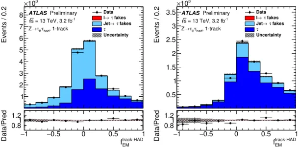
Figure 7: Fraction of EM energy from charged pions fEMtrack−HAD for one trackτhad−viscandidates before (left) and after (right) the medium identification requirement. fEMtrack−HADis defined as the fraction of the energy, deposited in the electromagnetic calorimeter, of tracks associated with theτhad−viscandidate in the core region. The uncertainty band contains only the statistical uncertainty.
Events / 0.05
1 10 102
103
104
105
106
ATLAS Preliminary = 13 TeV, 3.2 fb-1
s
, 1-track τhad
τµ
Z→
Data fakes τ l→
fakes τ Jet→ τ Uncertainty
iso track
f
0 0.2 0.4 0.6 0.8 1
Data/Pred
0.51 1.5
Events / 0.05
1 10 102
103
104
105
106
ATLAS Preliminary = 13 TeV, 3.2 fb-1
s
, 1-track τhad
τµ
Z→
Data fakes τ l→
fakes τ Jet→ τ Uncertainty
iso track
f
0 0.2 0.4 0.6 0.8 1
Data/Pred
0.51 1.5
Figure 8: Fraction of trackspTin the isolation region fisotrack for one trackτhad−viscandidates before (left) and after (right) the medium identification requirement. fisotrackis defined as the scalar sum of thepTof tracks associated with theτhad−viscandidate in the region 0.2<∆R<0.4 divided by the sum of thepTof all tracks associated with the τhad−viscandidate. The uncertainty band contains only the statistical uncertainty.