Lepton asymmetry from mixing and oscillations

MPP-2015-235; TUM-HEP-1018-15

Lepton asymmetry from mixing and oscillations

A. Kartavtsev

, P. Millington

and H. Vogel

a

Max-Planck-Institut f¨ur Physik,

F¨ohringer Ring 6, 80805 M¨unchen, Germany

b

Physik Department T70, Technische Universit¨at M¨unchen, James-Franck-Straße, 85748 Garching, Germany

c

School of Physics and Astronomy, University of Nottingham, Nottingham NG7 2RD, United Kingdom

E-mail: alexander.kartavtsev@mpp.mpg.de ,

p.millington@nottingham.ac.uk , hvogel@mpp.mpg.de

A

: We show how the two physically-distinct sources of CP-asymmetry relevant to sce- narios of leptogenesis: (i) resonant mixing and (ii) oscillations between different flavours can be unambiguously identified within the Kadanoff-Baym formalism. These contributions are isolated by analyzing the spectral structure of the non-equilibrium propagators without relying on the def- inition of particle number densities. The mixing source is associated with the usual mass shells, whereas the oscillation source is identified with a third intermediate shell. In addition, we identify terms lying on the oscillation shell that can be interpreted as the destructive interference between mixing and oscillation. We confirm that identical shell structure is obtained in both the Heisenberg- and interaction-picture realizations of the Kadanoff-Baym formalism. In so doing, we illustrate the self-consistency and complementarity of these two approaches. The interaction-picture approach in particular has the advantage that it may be used to analyze all forms of mass spectra from quasi- degenerate through to hierarchical.

K

: Kadanoff-Baym equations, Resonant Leptogenesis, lepton asymmetry

Contents

1 Introduction 2

2 Shell structure for two-particle mixing in the Heisenberg picture 4 3 Shell structure for two-particle mixing in the interaction picture 10

4 Comparison with the density matrix approximation 20

5 Comparison with the effective Yukawa approach 21

6 Phenomenological implications 24

7 Conclusions and outlook 31

A Non-equilibrium field theory 33

B Discrete symmetry transformations 39

C Rate equations in the radiation-dominated Universe 42

1 Introduction

Flavour mixing and oscillations provide two physically-distinct sources of CP-asymmetry, as has been observed experimentally in the neutral K, D, B and B

systems [1]. The physical relevance of these sources has also been identified (see e.g. refs. [2–6]) in the context of leptogenesis [7]

(for an overview, see e.g. [8]). Scenarios of leptogenesis provide a potential explanation for the observed baryon asymmetry of the universe, relying upon the existence of heavy right-handed Ma- jorana neutrinos, whose out-of-equilibrium decays in the early universe are able to produce a net lepton number. This lepton asymmetry is subsequently converted to the observed baryon asym- metry through the sphaleron processes of the standard electroweak theory. Whereas it is widely accepted that the mixing source is important for all mass spectra of the heavy neutrinos, the rela- tive importance of the oscillation source is still under debate. Even so, one would anticipate that oscillations are most relevant when the mass spectrum of the heavy neutrinos is quasi-degenerate, where it has long been recognized that flavour effects play a significant role both from the heavy- neutrino [9–18] and charged-lepton sectors [19–26]. Thus, one would expect flavour oscillations to provide a significant source of CP-asymmetry in scenarios of resonant leptogenesis [27–29].

In such models, heavy-neutrino self-energy effects dominate [30–32] and provide a resonant en- hancement of the leptonic CP-asymmetry, when the mass difference of at least two of the heavy neutrinos is comparable to their decay widths [27, 28]. In this context, it has recently been ob- served that the mixing and oscillation sources of lepton asymmetry are of equal magnitude and the same sign [4–6] (for a summary, see ref. [33]). This leads to a factor of two enhancement in the final lepton asymmetry, when both sources, rather than only one, are included. It remains an open question as to what extent these two distinct phenomena and the interplay between them are captured by competing approaches.

The impact of flavour oscillations can be accounted for through the quantum improvement of the classical Boltzmann equations by promoting the number densities of individual flavours to a matrix of densities [34], thereby allowing for flavour coherences. This approach yields the so- called density matrix formalism, which has been applied extensively to scenarios of leptogenesis [4, 5, 15, 18, 22, 35–40]. On the other hand, a semi-classical treatment of mixing is possible through the inclusion of effective Yukawa couplings [28, 29], which can account for the ε- and ε

-type CP violation, arising respectively from self-energy and vertex effects. Recently, there has been much progress in the literature [2, 3, 6, 41–63, 63–65] aiming to go beyond these semi-classical treatments and obtain ‘first-principles’ field-theoretic analogues of the Boltzmann equation. Often, these quantum transport equations are derived by means of the Kadanoff-Baym formalism [66, 67]

(for reviews, see refs. [68, 69]), itself embedded in the Schwinger-Keldysh [70, 71] closed-time path formalism (see also refs. [72–74]) of non-equilibrium thermal field theory. These approaches have the advantage that all quantum-mechanical effects are in principle accounted for consistently and systematically. However, an outstanding difficulty of such approaches is in the approximations needed to make the solution tractable and the extraction of physically meaningful observables. As a result, it is often not straightforward to compare directly the results of different analyses or to ascertain to what extent relevant physical effects are accounted for.

In this article, we illustrate how the mixing and oscillation sources can be unambiguously

identified in the Kadanoff-Baym formalism by means of the shell structure of the resummed heavy

neutrino propagators and independently of the definition of particle number densities. In the con- text of a toy two-flavour model, we will show that there are three distinct shells. Two of these shells correspond to mixing and can be associated with the quasi-particle mass shells, whereas the third, which can be identified with oscillations, lies at an intermediate energy. In addition, we identify terms lying on the oscillation shell that can be interpreted as the interference between oscillation and mixing. In so doing, we provide a further illustration of the interplay of these two effects in the generation of lepton asymmetry. Most significantly, we find that this interference is destructive.

With respect to the “benchmark” of the Boltzmann approximation (effective Yukawa couplings but flavour-diagonal number densities), this destructive interference can be viewed as a suppression of the oscillation source. Conversely, with respect to the “benchmark” of the density matrix approx- imation (tree-level Yukawa couplings but flavour-off-diagonal number densities), this destructive interference can be viewed as a suppression of the mixing source. This observation may in part account for apparent discrepancies between competing approaches and is anticipated to be of rel- evance to scenarios of resonant leptogenesis. Nevertheless, in spite of this destructive interference and in the weak-washout regime, we find that both oscillation and mixing sources can be of equal magnitude and contribute additively to the final asymmetry in agreement with the conclusions of refs. [4–6].

Aside from illustrating the interplay of these sources of CP-asymmetry, we perform the cal- culations in two very different approaches, namely the Heisenberg- and interaction-picture realiza- tions of non-equilibrium quantum field theory. In contrast to earlier approaches, the interaction- picture description introduced in ref. [75] (see ref. [76] for a summary) enables one to work in a perturbative loop-wise fashion without encountering so-called pinch singularities [77–83] or secular terms [69] thought previously to spoil such approaches to non-equilibrium field theory.

Quite remarkably, we find exact agreement between these two formulations, illustrating the self- consistency and complementarity of these two approaches. Working in the interaction-picture has the particular advantage that all forms of mass spectra can be analysed using a single method, from quasi-degenerate through to hierarchical.

In order to reduce the technical complications to a minimum and yet to include all qualitatively important effects for the generation of the asymmetry, we use a simple toy model studied previously in refs. [48, 49, 52, 63, 84, 85]. The model contains one complex and two real scalar fields:

L = 1

2 ∂

ψ

∂

ψ

− 1

2 ψ

M

ψ

+ ∂

¯ b ∂

b − m

¯ bb − λ

2!2! (¯ bb)

− h

2! ψ

bb − h

2! ψ

¯ b ¯ b , (1.1) where ¯ b denotes the Hermitian conjugate of b. Here and in the following, we assume summation over repeated indices, unless otherwise specified. Despite its simplicity, the model incorporates all features relevant for leptogenesis. The real scalar fields imitate the (two lightest) heavy right- handed neutrinos, whereas the complex scalar field models the leptons. The U (1) symmetry, which we use to define “lepton” number, is explicitly broken by the presence of the last two terms, just as the B − L symmetry is explicitly broken by Majorana mass terms in phenomenological models.

Thus, the first Sakharov condition [86] is fulfilled. The couplings h

model the complex Yukawa

couplings of the right-handed neutrinos to the charged-leptons and the Higgs doublet. By rephasing

the complex scalar field, at least one of the couplings h

can be made real. If arg(h

) 6= arg(h

),

the other one remains complex and there is C-violation, as is required by the second Sakharov condition.

The remainder of this article is organized as follows. Using the Heisenberg-picture realization of the Kadanoff-Baym formalism, we confirm in section 2 that the mixing and oscillation between different flavours indeed provide two distinct sources of lepton asymmetry. In section 3, we repeat the analysis in the interaction picture, finding identical results. Subsequently, in section 4, we make comparison with the density matrix approach and, in section 5, describe the inclusion of mixing effects via effective Yukawa couplings. Finally, in section 6, we discuss the phenomenological implications of these two sources of lepton asymmetry, as well as their interference, and present numerical results. Our conclusions are presented in section 7. In appendix A, we provide a brief outline of the details of the Kadanoff-Baym formalism pertinent to the analysis of this article. In addition, we summarize our definitions and notational conventions, making comparison with those that appear in the literature. In appendix B, we discuss the transformation properties of the model under generalized discrete symmetries and emphasize the need to specify C-symmetric initial con- ditions in the weak-washout regime. A derivation of the rate equations in an expanding Universe, relevant to the study of leptogenesis in the strong-washout regime, is presented in appendix C.

2 Shell structure for two-particle mixing in the Heisenberg picture

In this section, we show that the mixing and oscillation between different flavours provide two dis- tinct sources of lepton asymmetry, in agreement with arguments presented in refs. [4–6]. Whereas the standard mixing contributions [27, 29] are associated with the mass shells ω

(i = 1, 2) of the corresponding quasi-particles, the oscillation contribution is associated with a shell at ω ¯ = (ω

+ ω

)/2, which we refer to as the oscillation shell in the remainder of this paper. In or- der to identify this structure, we first analyze the generation of the lepton asymmetry using the Kadanoff-Baym equations in the Heisenberg picture, as were previously applied to the toy model from eq. (1.1) in ref. [63].

Asymmetry in the absence of washout. Following refs. [57, 63], we treat the complex scalar field as a thermal bath with temperature T and neglect the back-reaction. The system begins its evolution at t = − ∞ in an equilibrium state. At t = 0, it is brought out of equilibrium by an external source, thereby fulfilling the third Sakharov condition. This leads to a production of an asymmetry between the number densities of b and ¯ b. As time goes by, this asymmetry is erased by washout processes. Finally, at t = ∞, the system again reaches thermal equilibrium.

The washout processes are physically very important and must be taken into account in a phenomenological analysis. On the other hand, in the analysis limited to the source term alone, one can neglect them, as was previously done in refs. [57, 63]. In this approximation, the produced asymmetry is given by

η(t) = − 2 ImH

Z

−∞

dx

Z

−∞

dy

Z d

q (2π)

× i h

G

(x

, y

, q) Π

(y

, x

, q) − G

(x

, y

, q) Π

(y

, x

, q) i

, (2.1)

where H

≡ h

h

, the functions G

are components of the Wightman propagators of the real scalar fields ψ

, and Π

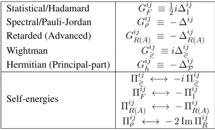
are the self-energies with the couplings “amputated”. A comprehensive summary of the various propagators and self-energies, their definitions and useful identities, as well as the differing nomenclature used throughout the literature is provided in appendix A.

The expression for the asymmetry in eq. (2.1) is derived by considering the conserved current of the complex scalar field (see ref. [63] for details of the derivation). This expression is entirely equivalent to the one obtained via the definition of the number densities used in the interaction- picture approach to the Kadanoff-Baym formalism, developed in ref. [75].

Solution of the Kadanoff-Baym equations. The Wightman propagators in eq. (2.1) are solutions to the Kadanoff-Baym equations for the mixing fields ψ

. In the absence of external sources, these transport equations read [49]

[

+ M

]G

(x, y) =

y⁰

Z

−∞

d

z Π

(x, z) G

(z, y) −

x⁰

Z

−∞

d

z Π

(x, z) G

(z, y) , (2.2)

where M

are the mass parameters of the renormalized Lagrangian, G

is the spectral function, and Π

and Π

are the Wightman and spectral self-energies, respectively. Using the definitions of the retarded and advanced propagators, and the self-energies in appendix A, we can rewrite eq. (2.2) in a form more convenient for the analysis that follows:

[

+ M

]G

(x, y) = − Z

z

h

Π

(x, z) G

(z, y) + Π

(x, z) G

(z, y) i

. (2.3) Here, we have introduced a compact notation R

z

≡ R

−∞

d

z. The Kadanoff-Baym equations for the retarded and advanced propagators can be derived from eq. (2.2):

[

+ M

]G

(x, y) = − Z

z

Π

(x, z) G

(z, y) + δ(x − y)δ

. (2.4) For our purposes, it is sufficient to know that, at the one-loop level to which we limit ourselves here, the self-energies of the real scalar fields are translationally invariant in the thermal bath. This implies, in particular, that eq. (2.4) admits a translationally-invariant solution. Using eq. (2.4), one can readily check that

G

(x, y) = − Z

u,v

G

(x, u) Π

(u, v) G

(v, y) (2.5) is a solution to eq. (2.3). Since, as is discussed above, the self-energies, as well as the retarded and advanced propagators on the rhs of eq. (2.5) are translationally invariant, the lhs of eq. (2.5) is also translationally invariant. In other words, eq. (2.5) is an equilibrium solution for the Wightman propagators.

In the setup considered here, the system is instantaneously brought out of equilibrium by an

external source at t = 0. The source can be considered as a bi-local contribution to the self-

energy. Following refs. [57, 63], we consider an external source that leaves the spectral func-

tion unperturbed. Thus, both of the Wightman self-energies are “perturbed” in the same way,

Π

(x, y) → Π

(u, v) − K

(u, v), with K

(u, v) = δ(u

)δ(v

)K

(u − v). The trans- lational invariance of the one-loop self-energies in the thermal bath renders the Kadanoff-Baym equations linear, i.e. a sum of two solutions is also a solution. Using this linearity, we obtain the following equation for the non-equilibrium part G

⊂ G

of the Wightman propagators induced by the external source:

[

+ M

]G

(x, y) = − Z

z

h

Π

(x, z) G

(z, y) − K

(x, z) G

(z, y) i

. (2.6)

Using eq. (2.4), one can readily check that [57, 63]

G

(x, y) = Z

u,v

G

(x, u) K

(u, v) G

(v, y) (2.7) is a solution to eq. (2.6). In the absence of expansion, we are only interested in the non-equilibrium part of the resummed Wightman propagators, which are common to both the positive and negative frequency components, G

= G

≡ G

. The sum of eqs. (2.5) and (2.7) gives the full solution of the Kadanoff-Baym equations in the thermal bath, as was studied in detail in ref. [63].

Shell structure of the non-equilibrium solution. The equilibrium solution in eq. (2.5) does not contribute to the asymmetry in agreement with the third Sakharov condition (see ref. [63] for more details) and will not be considered further. In order to unravel the shell structure of the non- equilibrium solution in eq. (2.7), we perform a Wigner transform (see appendix A). Using the relation between the double-momentum and Wigner representations [see eq. (A.9)] and neglecting sub-leading off-shell contributions (see ref. [63]), we obtain (for positive q

)

G

(t, q

> 0) ≈ Z

0

dp

2π

Z

0

dp

2π 2π δ q

−

(p

+ p

)

e

G

(p

) K

G

(p

) . (2.8) Note that all functions in eq. (2.8) depend on the common three-momentum q, which we omit for brevity in the remainder of this work. The explicit forms of the Wigner transforms of the retarded and advanced propagators can be inferred from eq. (2.4) using translational-invariance of the self- energies:

G

(q

) = − adjD

(q

)

det D

(q

) , (2.9)

where

D

(q

) ≡ q

δ

− M

− Π

(q

) . (2.10) Throughout this article, we use boldface for matrices in flavour space. We denote by Ω

the two zeros of det D

(q

) in the complex q

plane. To a good approximation, this determinant can be written as

det D

(q

) ≈ (q

− Ω

)(q

− Ω

) . (2.11)

The real and imaginary parts of Ω

,

Ω

= ω

+ i

2 Γ

, (2.12)

correspond to the in-medium frequency ω

and width Γ

, respectively. Having not needed to employ the gradient expansion, cf. refs. [83, 87], the leading self-energy corrections to the spectral structure of the non-equilibrium part of the propagator, specifically the shifts of the poles in the real and imaginary directions, have been taken into account. We would like to emphasize that eq. (2.11) is not only applicable, but actually becomes exact in the degenerate limit. The implications of this pole approximation for the effective regulator of the lepton asymmetry will be discussed later in the context of degeneracy symmetry limits (see e.g. ref. [4]).

Using Cauchy’s theorem to evaluate the integral approximately, we arrive at the advertised three-shell structure

G

(t, q

> 0) ≈ 1

|∆Ω

|

"

X

i=1

2π δ(q

− ω

)e

adjD

(ω

)

2ω

K

adjD

(ω

) 2ω

− 2π δ(q

− ω)e ¯

e

adjD

(ω

)

2ω

K

adjD

(ω

) 2ω

− 2π δ(q

− ω)e ¯

e

adjD

(ω

)

2ω

K

adjD

(ω

) 2ω

#

, (2.13)

where we have defined the average in-medium decay width Γ = ¯ 1

2 (Γ

+ Γ

) , (2.14)

and introduced

∆Ω

≡ Ω

− Ω

. (2.15)

In eq. (2.13), the three distinct shells are identified by the frequencies q

= ω

(i = 1, 2) and q

= ¯ ω ≡

(ω

+ ω

). The shells with frequencies q

= ω

lie at the two poles of the retarded propagator, which can be associated with quasi-particle degrees of freedom. As such, these terms correspond to the contribution from mixing. On the other hand, the additional intermediate shell with frequency q

= ¯ ω corresponds to the contribution from oscillations and, as we will see, the interference between mixing and oscillations. This three-shell structure matches that obtained in ref. [87], which makes use of a gradient expansion of the KB equations. Therein, the authors also find an additional fourth shell with frequency q

= ω

− ω

corresponding to particle-anti-particle coherences, which are not considered in the present analysis.

In order to gain a better understanding of the shell structure and to make comparisons with the

existing literature, we will now expand eq. (2.13) to first order in the self-energies. With regards to

the lepton asymmetry, we are only interested in the off-diagonal components of the non-equilibrium

part of the propagator. In the mass eigenbasis, in which the remainder of this article is understood,

these components read

G

(t, q

> 0) ≈ 2π δ(q

− ω

) 1

2ω

e

δn

(0) Π

(ω

)R

− 2π δ(q

− ω

) 1

2ω

e

δn

(0) Π

(ω

)R

+ 2π δ(q

− ω) ¯ 1

(2ω

)

(2ω

)

e

e

h

δn

(0) ∆M

− δn

(0)Π

(ω

) + δn

(0)Π

(ω

) i

R

. (2.16)

In eq. (2.16), ∆M

≡ M

− M

is the mass splitting, and we have employed the notation used in ref. [6]:

/i ≡

( 2 , i = 1

1 , i = 2 . (2.17)

In addition, for later convenience, we have introduced the following notation for the initial deviation of “particle number densities” from equilibrium:

δn

(0) ≡ K

(2ω

)

(2ω

)

. (2.18)

Note, however, that the identification of the mixing and oscillation shells in eq. (2.13) is indepen- dent of this definition. Finally,

R

≡ ∆M

(∆M

i/i

)

+ (ω

Γ

− ω

Γ

)

(2.19) is the effective regulator.

The first and second lines of eq. (2.16) live on the mass shells and describe the standard mixing contributions to the asymmetry. On the other hand, the third and fourth lines describe the contri- bution from oscillations and the interference between mixing and oscillations. In section 3, we will make use of the interaction-picture approach in order to isolate the interference terms from the pure oscillation terms. We note that the regulator eq. (2.19) cannot be applied naively in the doubly-degenerate limit M

→ M

and Γ

→ Γ

(for a comparison of various regulators in de- generacy symmetry limits, see e.g. refs. [4, 57]). Nevertheless, the last two terms of eq. (2.16) have structure similar to those of the i-th and /i-th mass shell terms, respectively, but with opposite signs.

Therefore, there is a partial cancellation of these contributions, an effect that becomes important in the maximally-resonant regime, where the interference between mixing and oscillations is antici- pated to be of most relevance. This cancellation has been analyzed in detail in refs. [57, 63], where it was demonstrated that, in the degenerate limit ω

→ ω

and Γ

→ Γ

, back-reaction of mixing on the oscillation ensures exact cancellation in agreement with the physical expectations.

Mixing and oscillation sources of CP asymmetry. It remains for us to study how each term of

eq. (2.16) contributes to the asymmetry by substituting it into eq. (2.1). As identified earlier, in

the absence of cosmological expansion, we are only interested in the non-equilibrium part of the

resummed Wightman propagators for which G

= G

= G

. In this case, the expression for the produced asymmetry [eq. (2.1)] simplifies to

η(t) = − 2 ImH

Z

0

dx

Z

0

dy

Z

q

G

(x

, y

, q) Π

(y

, x

, q) , (2.20) where we have taken into account that the system is brought out of equilibrium at t = 0 in the lower limits of the time integration. Next, we trade x

and y

for the central and relative coordinates t ≡

(x

+ y

) and R

≡ x

− y

. In addition, we use the Markovian approximation

2t

Z

−2t

dR

sin(R

q

) cos(R

p

) = 0 ,

2t

Z

−2t

dR

sin(R

q

) sin(R

p

) ≈ π δ(q

− p

) . (2.21) In this way, we may rewrite eq. (2.20) in the differential form

dη

dt = 4 Im H

Z

q0,q

θ(q

) Im G

(t, q

, q) Π

(q

, q) , (2.22) where we have restored the common momentum q and

Π

(q

, q) = 1

8π L

(q

, q) with L

(q

, q) = 1 + 2T

|q| ln

1 − e

1 − e

(2.23) (see ref. [63] for more details). Substituting the expression for G

from eq. (2.16) into eq. (2.22), we obtain the following expression for the time-derivative of the asymmetry:

dη

dt ≈ 2 X

i

Z

q

M

ω

e

δn

(0, q) Γ

(ω

, q)

(ω

, q) + 2 Im H

Im

Z

q

1 (ω

ω

)

e

e

Π

(¯ ω, q) h

δn

(0, q) ∆M

− δn

(0, q)Π

(ω

, q) + δn

(0, q)Π

(ω

, q) i

R

. (2.24)

The first line of eq. (2.24) originates from the mass shell terms of eq. (2.16) and describes the mixing source of lepton asymmetry. The second and third lines stem from the oscillation-shell terms of eq. (2.16) and contain the oscillation source and the interference between mixing and oscillations, which will be isolated in section 3.

Before concluding this section, we comment in more detail on the physical content of eq. (2.24).

Firstly, the overall factor of two arises because, in the toy model [eq. (1.1)], each decay of the heavy real scalar violates “lepton” number by two units. Secondly, we note that the mixing con- tribution has the standard structure [27, 29]. The asymmetry produced per unit time and unit volume is proportional to the departure from equilibrium δn

, the in-medium decay probability Γ

(ω

, q) = Γ

L

(ω

, q) and the in-medium asymmetry produced in each decay

= Im H

H

(M

− M

)M

Γ

(M

− M

)

+ (ω

Γ

− ω

Γ

)

L

(ω

, q) , (2.25)

where the function L

(ω

, q) takes into account quantum-statistical corrections to the decay width and C-violating parameter, respectively (see eq. (2.23) and refs. [48, 49]). Thirdly, the leading con- tribution to the oscillation term is proportional to δn

, as one might expect, sourcing asymmetry only in the presence of flavour coherences.

3 Shell structure for two-particle mixing in the interaction picture

In this section, we show how the shell structure identified above in the Heisenberg picture is repro- duced in the interaction picture.

Tree-level Wightman propagator. In the interaction-picture approach, the tree-level Wightman propagator can be obtained straightforwardly by evaluating the ensemble expectation value (EEV) of field operators directly (see appendix A and ref. [75]). In the double-momentum representation, it takes the form

G

(p, p

, ˜ t) = 2π|2p

|

δ(p

− M

) e

×

θ(p

, p

) δ

+ n

(t, p)

+ θ(−p

, −p

) n

(t, p)

(2π)

δ

(p − p

× 2π|2p

|

δ(p

− M

) . (3.1)

Here, we have distinguished, as is necessary in the interaction picture (see appendix A), between a macroscopic time t and a microscopic time ˜ t. In the end, the physical limit will be obtained at equal times X

= ˜ t (for more details, see ref. [75]).

Dressed Wightman propagator. In the Markovian approximation, the Schwinger-Dyson equa- tion of the Wightman propagator reduces to

G

(p, p

, ˜ t) = G

(p, p

, ˜ t) − G

(p) Π

(p)(2π)

δ

(p − p

) G

(p

)

− G

(p) Π

(p) G

(p, p

, ˜ t) − G

(p, p

, ˜ t) Π

(p

) G

(p

) , (3.2) and that of the retarded (advanced) propagator to

G

(p) = G

(p) − G

(p) Π

(p) G

(p) . (3.3) It was shown in ref. [6] that this system may be solved analytically for the resummed Wightman propagator, giving

G

(p, p

, ˜ t) = F

(p) G

(p, p

, ˜ t) F

(p

) − G

(p) Π

(p)(2π)

δ

(p − p

) G

(p

) , (3.4) where we have defined

F

≡ X

n= 0

h − G

· Π

i

= G

D

= − δ

+ G

Π

, (3.5a) F

≡

X

n= 0

h − Π

· G

i

= D

G

= − δ

+ Π

G

. (3.5b)

The second term on the rhs of eq. (3.4) describes equilibrium ∆L = 0 and ∆L = 2 scatterings.

Instead, the part of interest to us is contained within the first term on the rhs of eq. (3.4). In particular, we wish to study the part proportional to the deviation from equilibrium δn

(t, p).

Inserting the tree-level Wightman propagator from eq. (3.1) into eq. (3.4), this part is given by G

(p, p

, ˜ t)

= F

(p) 2π|2p

|

δ

(p

− M

)e

δn

(t, p)(2π)

δ

(p − p

)

× 2π|2p

|

δ

(p

− M

)F

(p

) , (3.6) in which

2π δ

(p

− M

) ≡ 2π θ(p

)δ(p

− M

) = 1 2E

i

p

− E

+ i − i p

− E

− i

, (3.7) and E

= (p

+ M

)

.

On-shell approximation. We will first illustrate that there is no contribution to the resummed non-equilibrium propagator in eq. (3.6) from the tree-level on-shell modes p

= M

. In so doing, we will also illustrate explicitly that eq. (3.6) is free of pinch singularities, which would potentially arise from ill-defined products of Dirac delta functions with identical arguments.

For this purpose, it is convenient to work with the Wigner transform (see appendix A) of the non-equilibrium part of the dressed Wightman propagator:

G

(q

> 0, X, ˜ t) = Z

Q0

e

F

(q

+ Q

/2)2π|2E

|

δ

(q

+ Q

/2)

− E

× δn

(t, q) 2π|2E

|

δ

(q

− Q

/2)

− E

F

(q

− Q

/2) , (3.8) where the trivial Q integral has been performed. Hereafter, we omit three-momentum arguments for notational brevity. In order to perform the Q

integral, we will now assume erroneously that the only poles are those provided by the Dirac delta functions appearing explicitly in eq. (3.8).

We emphasize that we should not anticipate obtaining the correct result, since G

also contain poles.

By virtue of the properties of the Dirac delta function, we may show that

|2E

|

δ (q

± Q

/2)

− E

= 2(2E

)

X

s=±1

δ Q

± 2q

∓ 2sE

(3.9)

Performing the integral over Q

, we then find

G

(q

> 0, X, t) = ˜ e

2π δ(q

− E

) F

(E

) δn

(t, q)

(2E

)

(2E

)

F

(E

) .

(3.10)

Equation (3.10) is finite and, in evaluating the tree-level poles, we have not encountered any singu-

lar behaviour, illustrating explicitly that the expression for the resummed propagator in eq. (3.6) is

free of pinch singularities.

One might be tempted to consider the terms in eq. (3.5) proportional to G

Π

and Π

G

as subleading. Were we to drop these contributions, we would find the following for the off- diagonal elements of eq. (3.10):

G

(q

> 0, X, ˜ t) = e

2π δ(q

− E) ¯ δn

(t, q)

(2E

)

(2E

)

. (3.11) Such an approximation for the resummed would-be heavy-neutrino propagator, when used in the equation for the asymmetry, discards the phenomenon of mixing, accounting only for oscillations between the two flavours, as identified in ref. [6]. In fact, as we will now show, the terms omitted in eq. (3.11) are of order unity, and G

(q, X, t) ˜ is identically zero due to the erroneous treatment of the pole structure in this on-shell approximation.

Given the explicit form of the dressed retarded propagator, we may show that G

(E

) Π

(E

) = ∆M

δ

+ [adj Π

(E

)]

det D

(E

) Π

(E

) . (3.12) The determinant in the denominator of eq. (3.12) can be written as

det D

(E

) = ∆M

Π

(E

) + det Π

(E

) . (3.13) Thus, we have

G

(E

) Π

(E

) = ∆M

Π

(E

) + δ

det Π

(E

)

∆M

Π

(E

) + det Π

(E

) , (3.14) where we have also used the fact that

[adj Π

(E

)]

Π

(E

) = δ

det Π

(E

) , (3.15) by definition of the adjugate matrix. We may then show that

G

(E

) Π

(E

) = δ

, Π

(E

) G

(E

) = δ

. (3.16) Substituting eq. (3.16) into the expression for the resummed propagator in eq. (3.10), it immedi- ately follows that it is identically zero. Clearly, this result is incorrect. As we will see, this is a consequence of having neglected the poles in G

.

Pole structure. The tree-level retarded (advanced) propagator has the form G

(p) = − δ

p

− M

± i sign(p

) = − P δ

p

− M

± iπδ

sign(p

)δ(p

− M

) , (3.17) where we have used the identity

1

x ± i = P 1

x ∓ iπδ(x) , (3.18)

in which P denotes the Cauchy principal value. Equation (3.18) may readily be confirmed by using the limit representations

δ(x) = lim

1 π

x

+

, P 1

x = lim

x

x

+

. (3.19)

Substituting eq. (3.17) into eq. (3.6), it would appear that we have products of Dirac delta functions of identical arguments. However, we have seen already that eq. (3.6) is free of pinch singulari- ties. The reason for this is that these pinch singularities are resummed, and it is by performing this resummation that we will obtain the correct form for the Wigner representation of the resummed Wightman propagator. In particular, both the equilibrium and non-equilibrium parts of the propa- gator acquire finite widths, cf. ref. [83].

In order to understand the structure of this resummation, it is helpful to begin with the single- flavour case. Therein, we wish to evaluate the following structure:

I

= X

n= 0

− G

· Π

2πδ(p

− M

) = X

n= 0

Π

p

− M

+ i sign(p

)

2πδ(p

− M

) . (3.20) We proceed by partial-fractioning the limit representation of the Dirac delta function:

2πδ(p

− M

) = i

p

− M

+ i − i

p

− M

− i . (3.21)

We may then treat the positive- and negative-frequency components of eq. (3.20) separately, writing I

= θ(p

)(I

− I

) + θ(−p

)(I

− I

) , (3.22) where

I

= i X

n= 0

Π

p

− M

+ i sign(p

)

1

p

− M

± i . (3.23)

For p

> 0, we find θ(p

)I

= iθ(p

)

∞

X

n= 0

P

1 p

− M

Π

+

∞

X

n= 0

(−Π

)

n! πθ(p

)δ

(p

− M

) , (3.24) where δ

(x) is the n-th derivative of the Dirac delta function. Herein, we have employed the distributional identity (see e.g. ref. [88])

1 x ± i

= P 1

x

∓ (−1)

(n − 1)! iπδ

(x) . (3.25)

The summation in the first term can be performed explicitly, and we obtain θ(p

)I

=

X

n= 0

P

iθ(p

)

p

− M

− Π

(p) + X

n= 0

(−Π

)

n! πθ(p

)δ

(p

− M

) . (3.26) Here, we have indicated that the remaining Cauchy principal value avoids the pole at p

= M

. Next, we write I

as

I

= iθ(p

)

∞

X

n= 0

Π

p

− M

+ i sign(p

)

P 1

p

− M

+ iπδ(p

− M

)

!

. (3.27) This particular separation of terms in eq. (3.27) is made in order to isolate the pinch-singular terms.

These arise from the product of poles at p

= M

+ i and p

= M

− i. The first term in

eq. (3.27) is finite and therefore the summation can be performed explicitly. This is not the case for problematic second term. However, spotting that this term is proportional to the original series I

, we obtain

θ(p

)I

= X

n= 0

P

iθ(p

)

p

− M

− Π

(p) − 1

2 θ(p

)I

. (3.28) Combining eqs. (3.26) and (3.28), we find

θ(p

)I

= X

n= 0

(−Π

)

n! πθ(p

)δ

(p

− M

) + 1

2 θ(p

)I

. (3.29) After proceeding analogously for the case p

< 0, we arrive at the result

I

=

∞

X

n= 0

(−Π

)

n! 2πδ

(p

− M

) = i

p

− M

+ i − Π

− i

p

− M

− i − Π

, (3.30) where the prescription is chosen here such that the contour of integration passes between the poles, all of which lie below the real axis. In this way, the rhs of eq. (3.30) is the complex delta function (see e.g. refs. [89, 90])

I

= 2πδ(p

− M

− Π

) , (3.31) which is well defined for any analytic test function and may also be understood in terms of the generalized Taylor series in the first equality of eq. (3.30). We see here that the resummation in the double-momentum representation has captured the leading self-energy corrections to the real and imaginary parts of the poles. Since we will ultimately be interested only in the poles for which Re p

> 0, we introduce the following generalization of eq. (3.7):

2πδ

(p

− M

− Π

) ≡ 1 2Ω

i

p

− Ω + i − i p

− Ω − i

, (3.32)

where Ω is the complex root of p

− M

− Π

= 0 with Re Ω > 0.

In the case of two flavours, the structure of the infinite series I

=

h

− G

· Π

i

2π δ(p

− M

) (3.33) is more complicated but nevertheless tractable. For definiteness, let us consider the form of this series for i = j = 1. In this case, each term must have the form

Π

p

− M

+ i sign(p

) · · · Π

p

− M

+ i sign(p

) . (3.34) The “· · · ” can then include any number of insertions of

Π

p

− M

+ i sign(p

) (3.35) or the pair

Π

p

− M

+ i sign(p

) · · · Π

p

− M

+ i sign(p

) . (3.36)

Between the latter, we may insert any number of occurrences of Π

p

− M

+ i sign(p

) . (3.37) We may quickly convince ourselves that this infinite series may be written in the form

I

=

∞

X

n= 0

1

p

− M

+ i sign(p

)

Π

+ Π

Π

p

− M

− Π

2π δ(p

− M

) . (3.38)

Proceeding in the same was as in the single-flavour case, this expression yields I

=

X

n= 0

1 n!

− Π

− Π

Π

p

− M

− Π

2π δ

(p

− M

) , (3.39)

which is formally equivalent to

δ([G

]

) = δ(det D

/[adj D

]

) ≡ [adj D

]

δ(det D

) , (3.40) where δ is understood to be the complex delta function. Thus, continuing similarly for the other components, we obtain the complete expression for the non-equilibrium part of the resummed propagator:

G

(p, p

, t) = [adj ˜ D

(p)]

2π|2p

|

δ

(det D

(p))

× δn

(p, t)(2π)

δ

(p − p

)2π|2p

|

δ

(det D

(p

))[adj D

(p

)]

. (3.41) In order to compare this result directly with the Heisenberg picture, we make the pole approx- imation in eq. (2.11). With this approximation, the complex delta function can be expanded as follows:

δ det D

(p)

= 1

∆Ω

δ(p

− Ω

) − δ(p

− Ω

)

. (3.42)

Note that this expression is only applicable for Ω

6= Ω

. In the doubly-degenerate case, the limit Ω

→ Ω

must be taken before the integral over p

.

In the equal-time limit X

= ˜ t, and using this approximation, the Wigner transform of eq. (3.41) is

G

(t, q

> 0) = 2πδ(q

− Ω

) [adj D

(Ω

)]

δn

(t, q)

|2Ω

|

|2Ω

|

|∆Ω

|

[adj D

(Ω

)]

.

(3.43)

Here, the sum over a, b = 1, 2 has been left implicit, Ω

≡ (Ω

+ Ω

)/2,

= 1 if a = b and

= −1 if a 6= b, and ∆Ω is as defined in eq. (2.15). Finally, performing the summations over a

and b, we find

G

(t, q

> 0) = 2πδ(q

− ω

) [adj D

(Ω

)]

δn

(t, q)

|2Ω

||∆Ω

|

[adj D

(Ω

)]

+ 2πδ(q

− ω

) [adj D

(Ω

)]

δn

(t, q)

|2Ω

||∆Ω

|

[adj D

(Ω

)]

− 2πδ(q

− Ω) [adj ¯ D

(Ω

)]

δn

(t, q)

|2Ω

|

|2Ω

|

|∆Ω

|

[adj D

(Ω

)]

− 2πδ(q

− Ω ¯

) [adj D

(Ω

)]

δn

(t, q)

|2Ω

|

|2Ω

|

|∆Ω

|

[adj D

(Ω

)]

, (3.44) where Ω = ¯ Ω

+ Ω

/2. It is essential to emphasize that the deviations from equilibrium δn

are the non-equilibrium parts of the physical dynamical number densities, which appear as unknowns in the interaction-picture propagators. Moreover, these are the spectrally-free number densities, which count excitations with energy E

.

In order to compare with eq. (2.16), we now expand eq. (3.44) to first order in Π

, yielding the following result for the off-diagonal components:

G

(t, q

> 0) ≈ 2π δ(q

− ω

) 1

2ω

δn

(t) Π

(ω

) R

− 2π δ(q

− ω

) 1

2ω

δn

(t) Π

(ω

) R

+ 2π δ(q

− ω) ¯ 1

(2ω

)

(2ω

)

h

δn

(t) ∆M

− δn

(t) Π

(ω

) + δn

(t) Π

(ω

) i

R

. (3.45) Thus, we find the following result for the asymmetry:

dη

dt ≈ 2 X

i

Z

q

M

ω

δn

(t, q) Γ

(ω

, q)

(ω

, q) + 2 Im H

Im

Z

q

Π

(¯ ω, q) (ω

ω

)

h

δn

(t, q) ∆M

− δn

(t, q)Π

(ω

, q) + δn

(t, q)Π

(ω

, q) i

R

. (3.46)

This closely resembles the Heisenberg-picture result in eq. (2.24), with the exception of the time- dependent phases. In order to show that the expressions for G

in eqs. (2.16) and (3.45) are in fact identical to first order in the self-energies, and by extension the expressions for the asymmetry in eqs. (3.46) and (2.24), we must now find the functional form of δn

(t) by solving the transport equations directly.

Before proceeding to do so, however, it is important to remark upon the role played by the

interference terms. These interference terms may now be distinguished from the pure oscillation

contribution. The former appear in the final line of eq. (3.46) and originate in the final line of

eq. (3.45), lying on the oscillation shell but being proportional to the diagonal components of

the time-dependent number densities. On the other hand, the oscillation contribution appears in the second line of eq. (3.46) and originates in third line of eq. (3.45), and is proportional to the off-diagonal components of the time-dependent number densities. This identification of the pure oscillation contribution is in accord with the conventions of refs. [4–6] and, as we will see below, it is subtly different to identifying the oscillation and interference contributions in terms of the components of the initial deviations from equilibrium, as appear in eq. (2.16), which makes sense only in the weak-washout regime.

We proceed by expanding all but the regulator structure in eq. (3.45) around ∆ω

= ω

−ω

= 0. At zeroth order, we find

G

(t, q

> 0) ⊃ 2πδ(q

− ω) ¯ 1

2¯ ω δn

(t)∆M

R

, (3.47) in which the mixing contributions have canceled and from which we see that the interference be- tween mixing and oscillations is destructive. At this point, one might be tempted to conclude that using the on-shell approximation for the heavy-neutrino propagator, cf. eq. (3.11), in the equation for the asymmetry is valid, and therefore that the approach of refs. [4–6], by including contributions from both mixing and oscillation, double-counts the final asymmetry. However, this is not the case.

Continuing to the next order in the expansion, we find G

(t, q) ≈ 2πδ(q

− ω) ¯ 1

2¯ ω δn

(t)∆M

R

− 2πδ(q

− ω) ¯ 1 2¯ ω

"

δn

(t) Π

(¯ ω)

4¯ ω

+ δn

(t) Π

(¯ ω) 4¯ ω

#

∆M

R

, (3.48) where the mixing terms are present, but are now suppressed by an additional factor of ∆M

. Here, we have neglected terms proportional to δ

(q

− ω) ¯ and Π

(¯ ω), which contribute sub-dominantly to the asymmetry. The asymmetry now takes the form

dη

dt ≈ 2 X

i

Z

q

M

¯

ω δn

(t, q) Γ

(¯ ω, q) ˜

(¯ ω, q) + 2 Im H

Z

q

Π

(¯ ω, q)

¯

ω Im δn

(t, q) ∆M

R

, (3.49) where the usual CP-violating parameter has been modified:

˜

(¯ ω, q) = ω

− ω

ω

+ ω

(¯ ω, q) . (3.50) Although both mixing and oscillation contributions persist in the middle-shell approximation and are clearly identifiable, in agreement with the results of refs. [4–6], we see that the structure of the mixing contribution has been modified. In addition to the suppression by an additional factor of

∆M

, a relative sign has emerged between the i = 1 and i = 2 contributions. As a result, the

modified mixing contribution is strongly suppressed when the deviations of the number densities

of the two flavours from equilibrium are similar. However, this is not always the case, for instance

in scenarios of resonant `-genesis [13, 14] (see also refs. [4–6]), where the lepton asymmetry is

dominantly produced in a single flavour through the decays of heavy neutrinos of a particular